Optimization of turning parameters by using design of experiments and simulated annealing algorithm based on audible acoustic emission signals

Abstract

The direct measurement of flank wear at regular intervals of time during machining consumes men and machine hours. This analysis focuses on the online monitoring of flank wear in turning from the experimentally observed audible acoustic emission signal. It is used as one of the indirect methods of monitoring flank wear in turning. The corresponding flank wear in all the test conditions for a machining time of 300 s are observed and recorded. When the value of the audible acoustic emission signal tends to reach the unsafe limit corresponding to the flank wear of above 0.2 mm, the operator is alerted to stop the operation to replace the tool. This technique minimizes the tool cost without sacrificing the quality of the final product. Also, this analysis inter-relates the performances of the design of experiments, regression analysis and simulated annealing algorithm to obtain the best possible solution. The result of this analysis identifies the optimal values of selected parameters for effective and efficient machining. The experimental, optimized and predicted values of flank wear are compared and correlated with the experimental audible acoustic emission signal.

Introduction

The replacement of cutting tools is the major portion of cost of production in all the manufacturing industries. The surface roughness of the finished components depends particularly on the bluntness of the cutting tool.

In the past few decades, a variety of tool wear identifying techniques have been established that are used effectively for the detection of tool failure. The progress of tool wear has been measured by using optical techniques such as a TV camera ¹ or a charged coupled device (CCD) camera. ² Even though several models^3–6 have been developed to predict cutting tool life, owing to the complexity of machining processes none of these are universally successful. The importance of sensing technology has been pointed out in all these studies in the development of flexible manufacturing systems.

Rantatalo et al. ⁷ used the non-contact laser Doppler vibrometer to investigate the behavior of a high-speed rotating system. Nakagawa et al. ⁸ also used the laser Doppler vibrometer to monitor chatter vibration in the end milling process online. Prasad et al. ⁹ have developed a system for monitoring the condition of the tool using an acousto-optic emission signal in face turning.

Iturrospe et al. ¹⁰ used a bicep strum-based blind system identification technique for estimating both the transmission path and sensor impulse response of acoustic emission (AE) signals. Yamaguchi et al. ¹¹ made detailed investigations of the cutting force and AE measured during the diamond turning process. Marinescu and Axinte ¹² used the AE signal for monitoring both tool and workpiece surface integrity to enable milling of the “damage-free” surfaces. Guo and Ammula ¹³ developed a practical online AE monitoring system for surface integrity in hard machining. JemieIniak et al. ¹⁴ used the wavelet packet transform (WPT) for extracting tool condition monitoring (TCM) features from the cutting forces and AE signals during turning of Inconel 625.

Hamdan et al. ¹⁵ used the Taguchi optimization technique in high-speed machining to identify the optimal control factors that yield the lowest cutting force and surface roughness. Zhang et al. ¹⁶ used the Taguchi design method for surface roughness optimization in end milling. Yang and Tamg ¹⁷ found the optimal cutting parameters in turning based on the Taguchi method

Conventional optimization techniques, like the full factorial method, Taguchi’s design of experiments (DoE), etc., are useful only for specific optimization problems that need only the best levels of parameters for the calculation of a local optimal solution. Consequently, non-traditional optimization techniques, such as a genetic algorithm, simulated annealing algorithm (SAA), particle swarm optimization (PSO) technique, etc., were used in the optimization problem to obtain the global solution. Yang and Natarajan ¹⁸ carried out experimental work in optimizing the machining parameters for the minimization of flank wear (FW) and cutting zone temperature. Bharathi Raja and Baskar ¹⁹ determined the optimized cutting parameters using the PSO technique. Vijayakumar et al. ²⁰ used the ant colony system for the optimization of multi-pass turning operations. The optimization problem in turning has been solved by genetic algorithms, Tabu search, simulated annealing and PSO to obtain more accurate results by Milfelner et al. ²¹ Sardinas et al. ²² optimized cutting parameters in the turning process genetic algorithm. Asokan et al. ²³ optimized the surface grinding operations using the PSO technique. The application of PSO in the scheduling of flexible manufacturing systems have been studied by Jerald et al. ²⁴

Khan et al. ²⁵ concluded in their experimental work that the simulated annealing technique and genetic algorithm are reliable and accurate for solving machining optimization problems over gradient-based methods. Tang et al. ²⁶ used an adaptive genetic algorithm for resource allocation in multiuser packet-based orthogonal frequency division multiplexing systems. Garg ²⁷ compared the memetic algorithm and genetic algorithm and investigated the performance for cryptanalysis on simplified data encryption standard problems. So many optimization techniques were applied for the optimization of cutting parameters in machining of various materials, but most of the approaches have not been focused towards the selection of a practically used machine component as a specimen as well as towards presenting the results of the DoE, regression analysis and SAA together.

This study focuses on the online monitoring of FW during turning based on the experimentally observed audible AE signal. The results of the analyses obtained by the said techniques are correlated with the experimental values. Four different power transmission shafts, such as the Ashok Leyland lorry axle, Ambassador car axle, Mahindra Tractor axle and Mahindra jeep axle, with hardness values in Brinell Hardness Number (BHN) of 110 BHN, 35 BHN, 65 BHN and 45 BHN respectively, are selected as specimens for machining. Uncoated cemented carbide cutting inserts of the same specification (CNMG 120408) are used for all machining operations. The process and product parameters selected for machining are, material hardness (H), cutting speed (V), feed rate (f) and depth of cut (d).

Optimization and modeling tools used

The tools used in this study are, Taguchi’s DoE and SAA for optimization and regression analysis for developing empirical models.

Taguchi’s DoE

An objective function is formulated with constraint to identify the optimal levels of cutting parameters using Taguchi’s DoE. The selected parameters, such as material hardness, cutting speed, feed rate and depth of cut, is varied through four levels within the recommended machining values. The optimization of process and product parameters considerably improves the quality characteristics. When the number of parameters and levels increase, a large number of experiments are required to be conducted. In order to reduce the number of experiments to be conducted for the same number of parameters and levels, the Taguchi’s DoE employs a specially designed orthogonal array to study the entire parameter levels with a conduct of the minimum number of experiments and is calculated as

$$\text{Minimum number of experiments}=[(\text{L}-1)\times \text{P}]+1=[(4-1)\times 4]+1=13\approx {\text{L}}_{16}$$

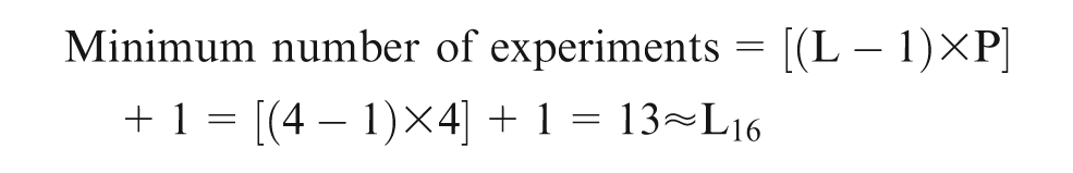
where L is the number of levels of parameters and P is the number of parameters.

In order to normalize the data, signal-to-noise (S/N) ratio values of AE and flank wear (FW) are calculated. The S/N ratio for AE, FW and surface roughness is calculated as

$$\text{S}/\text{N Ratio}=-10{\log }_{10}\frac{1}{n}\sum \stackrel{-}{y^2}$$

(1)

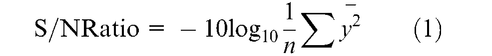
where n is the number of serials of experiment and $\overline{y}$ is the sum of squares of measured data.

Since the objective of this analysis is to minimize the audible AE and FW, lower-the-better category is selected to calculate the S/N ratio. Since the S/N values are used, the larger value is normally taken as a better performance characteristic. Therefore, the highest value of S/N ratio identifies the optimal level of the particular parameter. Also, the surface roughness is fixed as the constraint and the value of surface roughness of the finished component is not allowed to exceed 5 microns. ²⁸ Finally, a validation experiment is conducted with all the identified optimal levels of the parameters to confirm the optimality.

Regression analysis

The objective of linear regression is to create a prediction equation that expresses any output ‘y’ as a function of the independent variables. If the independent variables are measured, then the values can be substituted and the prediction for ‘y’ can be obtained. The non-linear regression is an extension of simple linear regression to allow for more than one independent variable. That is, instead of using only one independent variable, ‘x’, to explain the variation in ‘y’, several independent variables can be used. By using more than one independent variable, the accurate prediction of ‘y’ is possible. ²⁹

In order to compare the results of prediction obtained using linear regression and non-linear regression, “regression analysis” is used to develop the linear and non-linear empirical models based on experimental audible AE and FW values. The audible AE values predicted by the linear and non-linear regression models are correlated with the experimental audible AE values and the relative trend is analyzed.

Often, the problem of analyzing the quality of the estimated regression line is handled by an analysis-of-variance (ANOVA) approach. It is a procedure whereby the total variation in the dependent variable is subdivided into meaningful components that are then observed and treated in a systematic fashion. ³⁰ Fnides et al. ³¹ used the ANOVA technique and states that a low p value (<0.05) ANOVA indicates a statistical significance for the source on the corresponding response (i.e. 95% confidence level). Kazancoglu et al. ³² used the ANOVA technique and obtained quantitatively the significance of factors on overall quality characteristics of the cutting process.

SAA

The SAA simulates the slow cooling process to achieve the minimum function value in a minimization problem. The cutting parameters are introduced with the concept of Boltzmann probability distribution and the cooling phenomenon is simulated. Simulated annealing is a point-by-point method. The algorithm begins with an initial point and a high temperature ‘T’. A second point is created at random in the vicinity of the initial point and the difference in the function values ( $\Delta$ E) at these two points is calculated. If the second point has a smaller function value, then that point is accepted with the probability of exp(– $\Delta$ ET^−.1). This completes an iteration of this simulated annealing procedure. In the next generation, another point is created at random in the neighborhood of the current point and the Metropolis algorithm is used to accept or reject the point.

The Metropolis algorithm is a widely used procedure for sampling from a specified distribution on a large finite set. It is a procedure for drawing samples from finite set x. ³³ A considerable amount of attention is now being devoted to the Metropolis algorithm, which was developed by Metropolis et al. ³⁴ and subsequently generalized by Hastings. ³⁵ In order to simulate the thermal equilibrium at every temperature, the number of points (n) is usually tested at a particular temperature, before reducing the temperature. The algorithm is terminated when a sufficiently small temperature is obtained or a small enough change in the function values is found. The steps of the SAA are shown in Figure 1.

Figure 1.

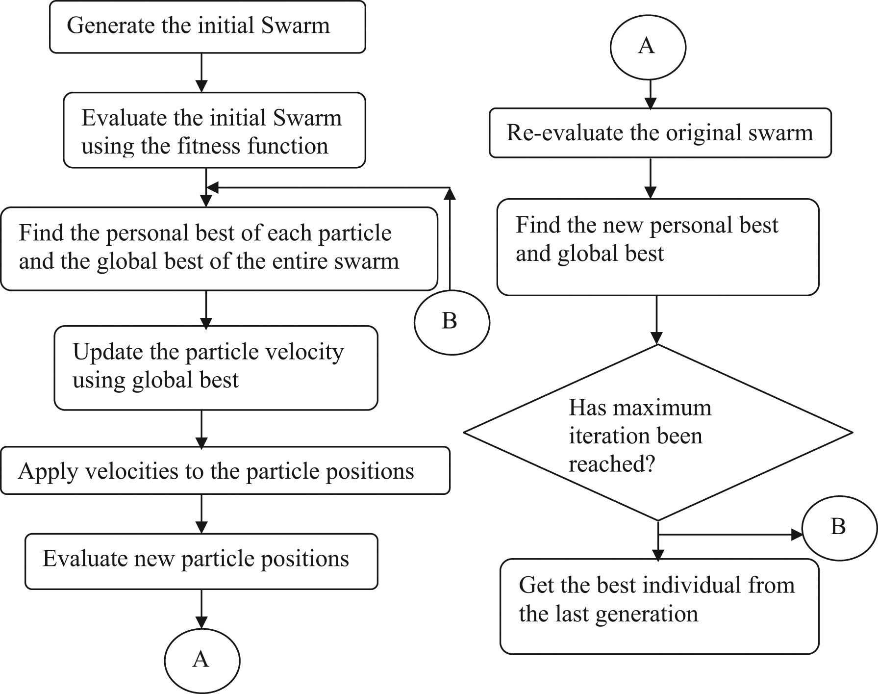
Flow chart of the SAA.

Experimental details

Turning with a single-point cutting tool is one of the widely used machining operations in most of the manufacturing industries. Material hardness, cutting speed, feed rate and depth of cut were selected as parameters and the FW was selected as a performance quality characteristic.

The test was carried out using a computer numerically controlled (CNC) lathe for a machining duration of 300 s, irrespective of the number of passes in order to avoid chipping and blending of the tool. A stereo microphone was fitted on the tool post of the CNC lathe at a constant distance of 50 mm from the cutting zone with the help of a vibration damping clamp.

Since the unavoidable machine noises play a negligible and uniform role throughout the process, no precautions were taken to avoid or to measure the non-relevant ambient noises generated by the machine. The continuous electrical signals generated by the stereo microphone during machining were transferred to the SEAWAVE Software. The default effective sampling rate of 32,000 samples/s was used with the installed audio controller of Intel 82801DB I/O for all the test conditions.

The peak value of the audible AE signal during the machining time was observed and recorded manually for all the test conditions. The experimental setup, with details is shown in Figure 2(a) and the exploded view showing the vibration damping clamp that has been tightly fitted between the tool post of CNC lathe and the microphone, is shown in Figure 2(b).

Figure 2.

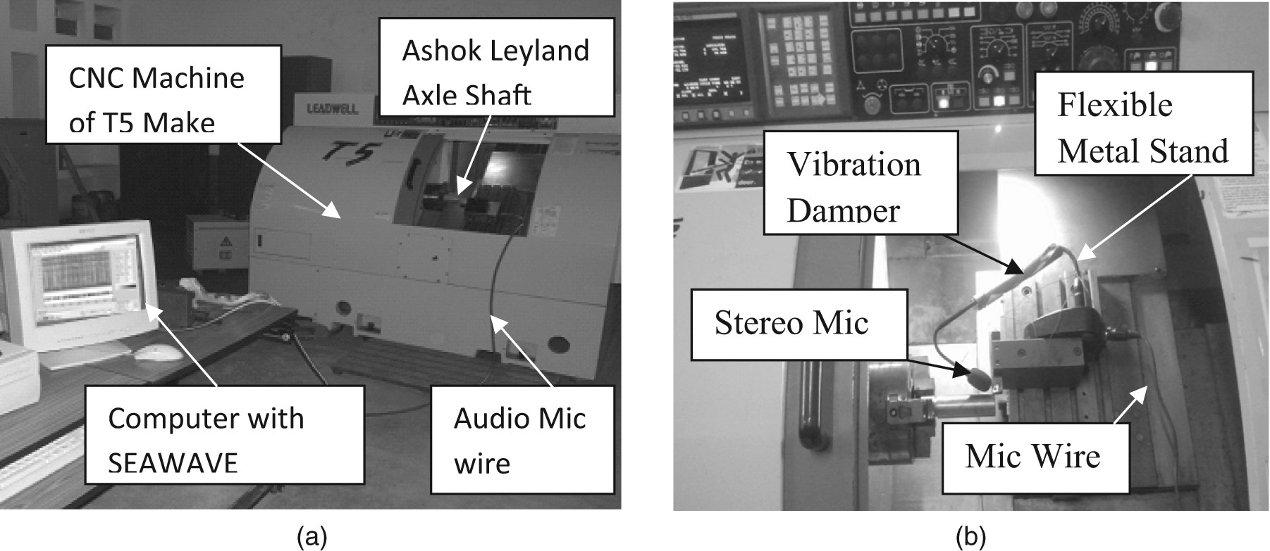
(a) Experimenal set up; (b) exploded view of microphone setup.

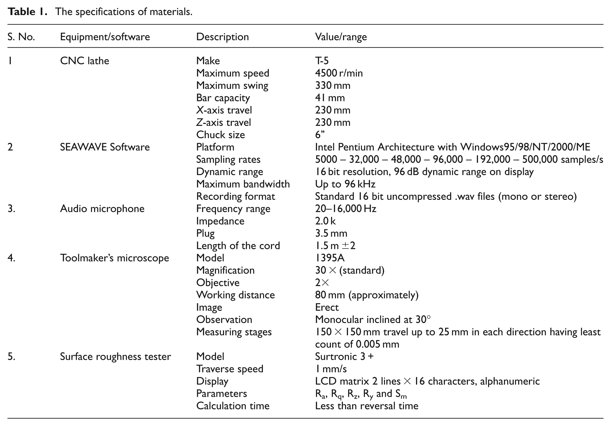
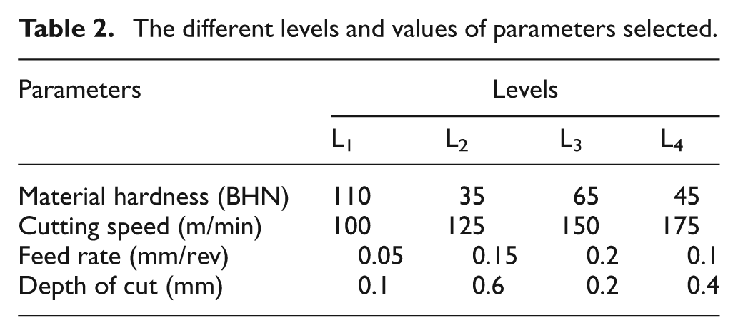
The specifications of CNC lathe, software used for recording the electrical signals from the microphone, audio microphone, tool maker’s microscope and surface roughness tester are presented in Table 1. The values of various cutting parameters are selected based on the data given in the machining handbook, and are presented in Table 2. Each experiment was conducted as per the test conditions shown in Table 3 using different fresh cutting edges of the same specifications for a convenient continuous machining duration of 300 s in order to avoid chipping of the tool.

Table 1.

The specifications of materials.

S. No.	Equipment/software	Description	Value/range
1	CNC lathe	Make	T-5
		Maximum speed	4500 r/min
		Maximum swing	330 mm
		Bar capacity	41 mm
		X-axis travel	230 mm
		Z-axis travel	230 mm
		Chuck size	6”
2	SEAWAVE Software	Platform	Intel Pentium Architecture with Windows95/98/NT/2000/ME
		Sampling rates	5000 – 32,000 – 48,000 – 96,000 – 192,000 – 500,000 samples/s
		Dynamic range	16 bit resolution, 96 dB dynamic range on display
		Maximum bandwidth	Up to 96 kHz
		Recording format	Standard 16 bit uncompressed .wav files (mono or stereo)
3.	Audio microphone	Frequency range	20–16,000 Hz
		Impedance	2.0 k
		Plug	3.5 mm
		Length of the cord	1.5 m ±2
4.	Toolmaker’s microscope	Model	1395A
		Magnification	30 × (standard)
		Objective	2×
		Working distance	80 mm (approximately)
		Image	Erect
		Observation	Monocular inclined at 30°
		Measuring stages	150 × 150 mm travel up to 25 mm in each direction having least count of 0.005 mm
5.	Surface roughness tester	Model	Surtronic 3+
		Traverse speed	1 mm/s
		Display	LCD matrix 2 lines × 16 characters, alphanumeric
		Parameters	Ra, Rq, Rz, Ry and Sm
		Calculation time	Less than reversal time

Table 2.

The different levels and values of parameters selected.

Parameters	Levels
	L1	L2	L3	L4
Material hardness (BHN)	110	35	65	45
Cutting speed (m/min)	100	125	150	175
Feed rate (mm/rev)	0.05	0.15	0.2	0.1
Depth of cut (mm)	0.1	0.6	0.2	0.4

Table 3.

Experimental test conditions and parameter values.

Test condition number	Hardness H (BHN)	Cutting speed V (m/min)	Feed rate f(mm/rev)	Depth of cut d (mm)
1	110	100	0.05	0.1
2	110	125	0.15	0.6
3	110	150	0.2	0.2
4	110	175	0.1	0.4
5	35	100	0.1	0.2
6	35	125	0.2	0.4
7	35	150	0.15	0.1
8	35	175	0.05	0.6
9	65	100	0.15	0.4
10	65	125	0.05	0.2
11	65	150	0.1	0.6
12	65	175	0.2	0.1
13	45	100	0.2	0.6
14	45	125	0.1	0.1
15	45	150	0.05	0.4
16	45	175	0.15	0.2

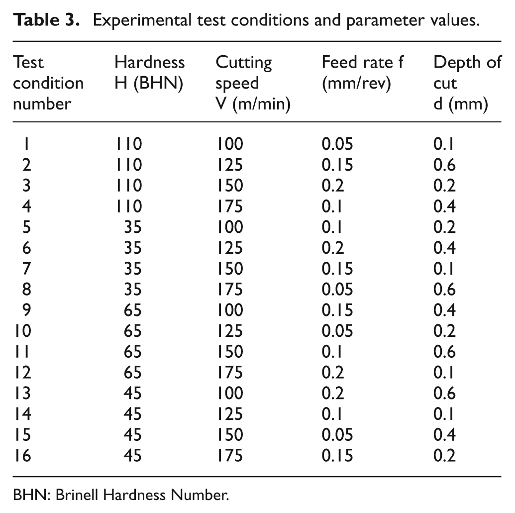
BHN: Brinell Hardness Number.

The peak values of the audible AE signal were recorded during machining time for all 16 experiments. The snapshot of the value of the audible AE signals recorded using SEAWAVE software during machining is shown in Figure 3. At the end of each experiment, the FW values of the cutting inserts were measured and recorded by using a tool maker’s microscope (specifications as shown in Table 1). Later the S/N ratio values of the FW were calculated using equation (1). The surface roughness of the finished product was measured by using a surface roughness tester (specifications as shown in Table 1).

Figure 3.

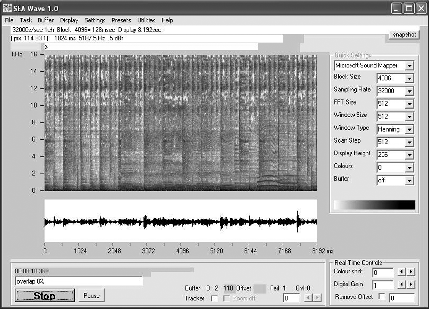
Snapshot of SEAWAVE software window during recording of the audible AE signals.

The surface roughness tester showed three parameter values of surface roughness, like arithmetic average deviation (R_a), peak-to-peak height (R_y) and root mean square average (R_z). The arithmetic average deviation is the average absolute value of profile excursions from the mean line. Usually R_a is measured five times (over consecutive values of sampling length L) and an average is calculated. ³⁶

The American National Standards Institute specifies the arithmetic average deviation as the standard unit for surface roughness. ³⁷ Hence, only the arithmetic average deviation (R_a) was observed, recorded and taken into consideration for the analysis. The S/N ratio of surface roughness was calculated using equation (1).

Results and discussions

According to Taguchi’s DoE, the minimum number of experiments for the selected parameters were conducted. The peak values of audible AE signals, FW and surface roughness corresponding to each experiment were recorded. The experimental test conditions and observed data (both raw and S/N values) are presented in Table 4. The value of the S/N ratio for FW and audible AE was calculated using equation (1) for test condition number 5 as

$$\text{S}/\text{N ratio of FW}=-10{\log }_{10}(65\times 65)=-36.2583$$

$$\text{S}/\text{N ratio of AE}=-10{\log }_{10}(57.03\times 57.03)=-35.1221$$

Table 4.

Observed experimental data and test results.

Test condition number	FW (µm)	AE (db)	Ra (µm)	S/N–FW	S/N–AE	S/N–Ra
1	105	94.41	1.08	−40.42	−39.50	−40.66
2	80	68.52	0.82	−38.06	−36.71	−38.27
3	95	76.55	0.93	−39.55	−37.67	−39.36
4	75	66.13	0.79	−37.50	−36.40	−37.95
5	65	57.03	0.66	−36.25	−35.12	−36.39
6	70	62.55	0.76	−36.90	−35.92	−37.61
7	60	55.72	0.64	−35.56	−34.92	−36.12
8	50	40.53	0.49	−33.97	−32.15	−33.80
9	75	64.33	0.8	−37.50	−36.16	−38.06
10	65	56.45	0.69	−36.25	−35.03	−36.77
11	65	54.93	0.71	−36.25	−34.79	−37.02
12	70	59.66	0.75	−36.90	−35.51	−37.50
13	55	44.23	0.6	−34.80	−32.91	−35.56
14	55	48.25	0.57	−34.80	−33.66	−35.11
15	50	36.55	0.49	−33.97	−31.25	−33.80
16	50	39.33	0.54	−33.97	−31.89	−34.64

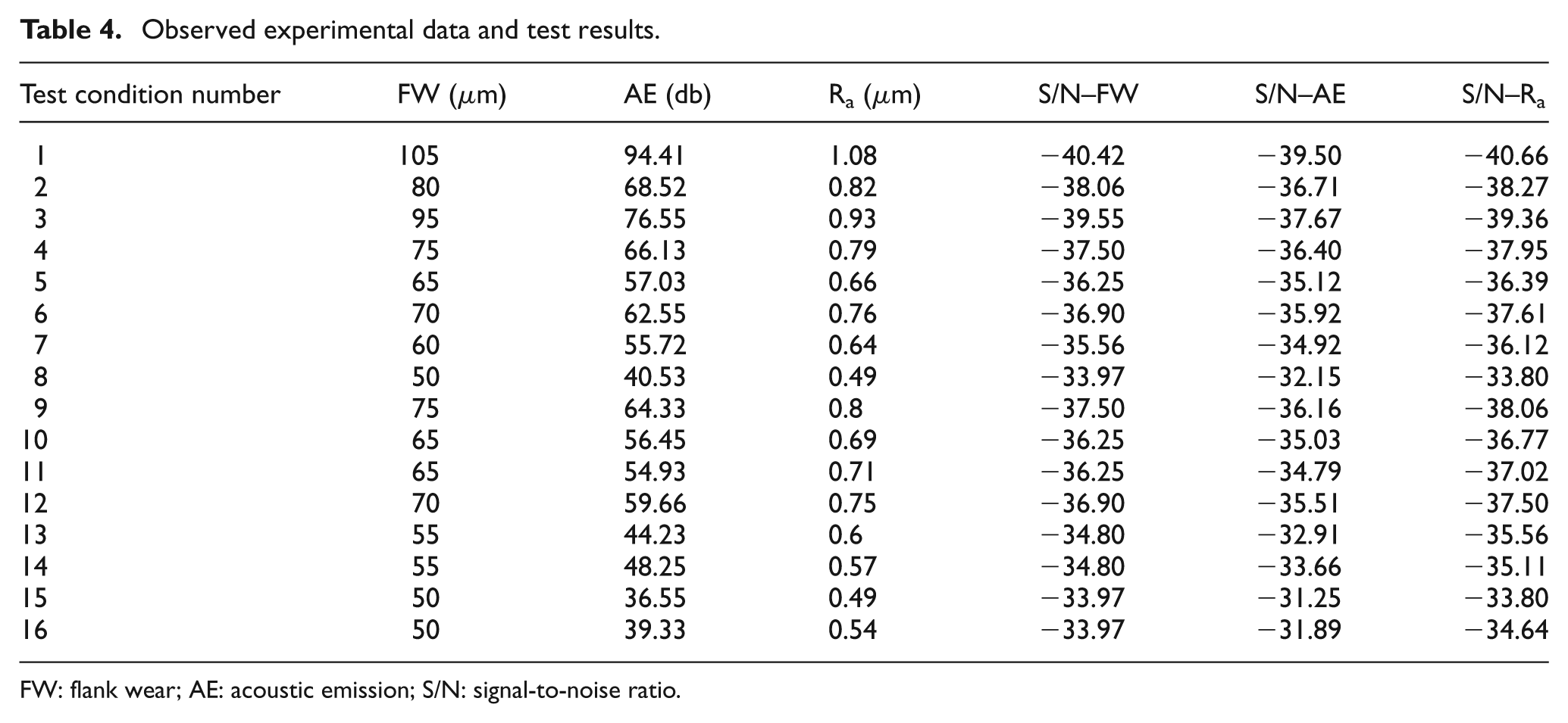
FW: flank wear; AE: acoustic emission; S/N: signal-to-noise ratio.

The best level of parameters (maximum value of S/N ratio) were identified as

$$\text{Hardness of workpiece}=45\text{BHN}\left({\text{H}}_4\right)$$

$$\text{Cutting speed}=175\text{m}/\text{min}\left({\text{V}}_4\right)$$

$$\text{Feed rate}=0.05\text{mm}/\text{rev}\left({\text{f}}_1\right)$$

$$\text{Depth of cut}=0.6\text{mm}\left({\text{d}}_2\right).$$

With the identified best level of parameters, a validation experiment was conducted for obtaining the minimum value of FW based on the audible AE signal. The value of audible AE and FW values were 45 microns and 36.52 db, respectively, which were lower than all the test condition values. The corresponding S/N ratio results of the validation experiment are shown below as

$$\text{Audible AE signal}=-31.2506$$

$$\text{FW}=-33.0643$$

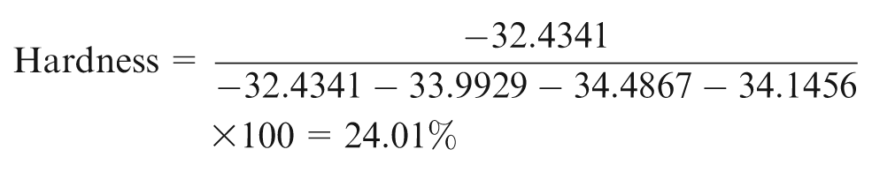
From Table 4, the percentage contribution of parameters on S/N-audible AE was calculated as

$$\text{Hardness}=\frac{-32.4341}{-32.4341-33.9929-34.4867-34.1456}\times 100=24.01\%$$

$$\text{Cutting speed}=25.16\%$$

$$\text{Feed rate}=25.53\%$$

$$\text{Depth of cut}=25.28\%$$

Similarly the percentage contribution of parameters on S/N-FW was calculated and found as

$$\text{Hardness}=24.23\%$$

$$\text{Cutting speed}=25.07\%$$

$$\text{Feed rate}=25.47\%$$

$$\text{Depth of cut}=25.2\%$$

From the above calculations, it is confirmed that the material hardness is less significant on the S/N–audible AE and S/N–FW followed by other parameters. The feed rate is highly significant on S/N–audible AE and S/N–FW.

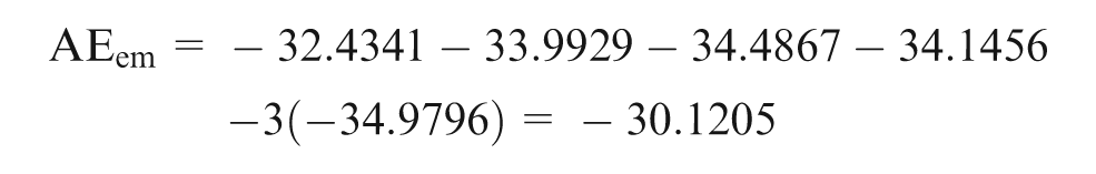
For verifying the validated results of audible AE signals based on the linear regression model, the estimated mean of audible AE was calculated as

$${\text{AE}}_{\text{em}}=\text{H}+\text{V}+\text{f}+\text{d}-3\text{A}{\text{E}}_{\text{m}}$$

(2)

where AE_em is the estimated mean of audible AE, H is the mean of audible AE corresponding to hardness, V is the mean of audible AE corresponding to cutting speed, f is the mean of audible AE corresponding to feed rate, d is the mean of audible AE corresponding to depth of cut and AE_m is the overall mean of audible AE.

From Table 4, the mean values of the parameters were substituted in equation (2) and the estimated mean of audible AE was calculated as

$${\text{AE}}_{\text{em}}=-32.4341-33.9929-34.4867-34.1456-3(-34.9796)=-30.1205$$

The linear regression data for audible AE was developed by using regression analysis, as shown in Table 5.

Table 5.

Summary output – linear regression – acoustic emission.

	df	SS	MS	F	Significance F
Regression	4	54.84	13.71	8.421546	0.0023077
Residual	11	17.91	1.628
Total	15	72.75
	Coefficient	Standard error	t stat	p-value
Intercept	−35.2671	1.96	−17.94	1.71E-09
H	−0.0546	0.011	−4.93	0.000449
N	0.025891	0.011	2.268	0.044418
f	−5.97837	5.706	−1.047	0.317274
d	2.940647	1.661	1.77	0.104371

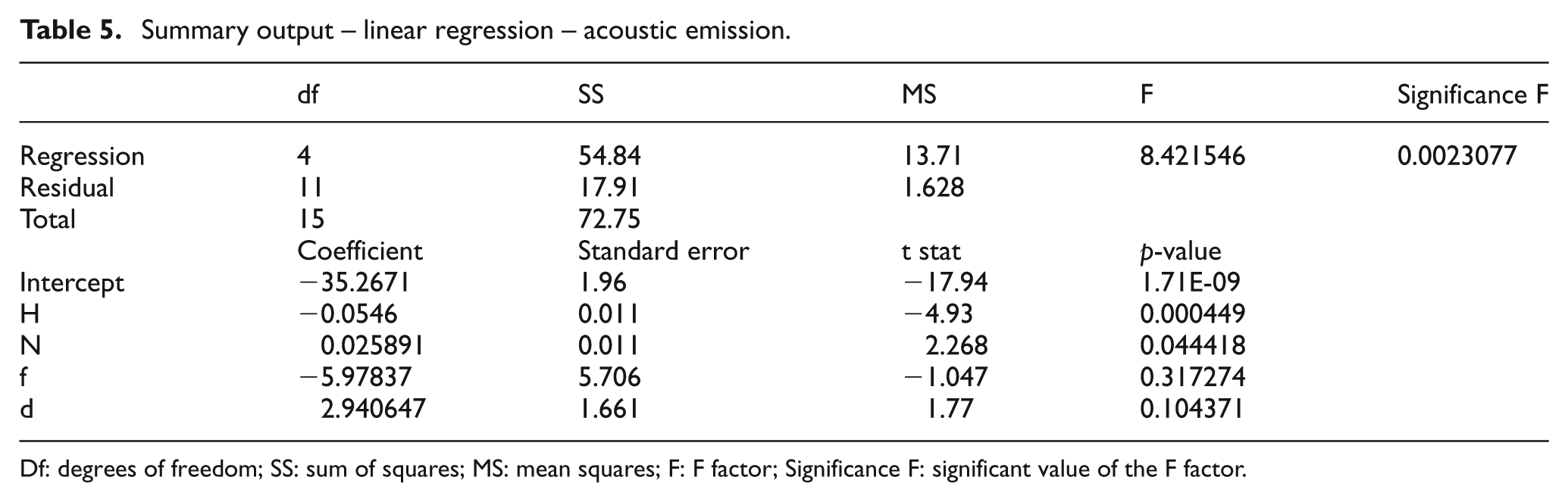
Df: degrees of freedom; SS: sum of squares; MS: mean squares; F: F factor; Significance F: significant value of the F factor.

A confidence interval (CI) of 95% for the prediction of audible AE based on the validation experiment on the basis of linear regression model is presented as

$$\mathrm{CI}=\sqrt{F_0.05(3,f_e)V_e[\frac{1}{n}+\frac{1}{R}]}$$

(3)

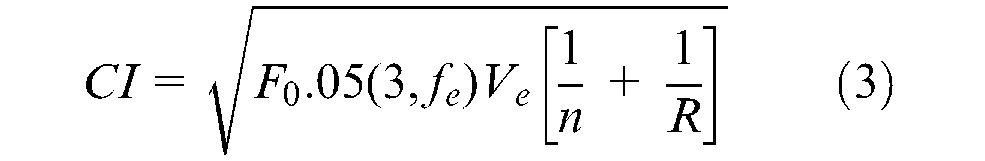
where f_e is the error degrees of freedom (11) from Table 5, F_0.05 (3, f_e) is the F ratio required for risk (3, 11) = 8.76 from standard “F” table, ³⁸ Ve is the error variance (1.628) from Table 5, R is the number of repetitions for confirmation test (1), N is the total number of experiments (16), and n is the effective number of replications = N/(1 + degrees of freedom associated with audible AE) = 16/(1 + 15) = 1.

By substituting the above values in equation (3), the value of confidence interval for audible AE based on linear regression model is calculated as

$$\text{CI}={\{8.76\times 1.628[(1/1)+(1/1)]\}}^{1/2}=5.3406$$

The 95% confidence interval for the optimal audible AE in validation experiment is verified as

$$(\text{A}{\text{E}}_{\text{em}}-\text{CI})<\text{A}{\text{E}}_{\text{con}}<(\text{A}{\text{E}}_{\text{em}}+\text{CI})=(-30.1205-5.3406)<\text{A}{\text{E}}_{\text{con}}<(-30.1205+5.3406)=-35.4611<\text{A}{\text{E}}_{\text{con}}<-24.7799$$

The result of the validation experiment shows that the audible AE is −31.2506, which is in between −35.4611 and −24.7799. The validated audible AE is thus confirmed by the above calculations. The linear regression model values are shown in Table 6.

Table 6.

Linear regression model values.

Test condition number	S/N–FW	S/N–AE	LR–FW	%error LR–FW	LR–AE	% error LR–AE
1	−40.42	−39.50	−39.62	2.02	−38.68	2.09
2	−38.06	−36.71	−38.69	1.64	−37.16	1.21
3	−39.55	−37.67	−39.35	0.50	−37.99	0.83
4	−37.50	−36.40	−37.71	0.55	−36.16	0.67
5	−36.25	−35.12	−35.72	1.49	−34.59	1.51
6	−36.90	−35.92	−35.43	4.12	−33.96	5.78
7	−35.56	−34.92	−35.20	1.02	−33.89	3.01
8	−33.97	−32.15	−32.91	3.22	−31.18	3.12
9	−37.50	−36.16	−37.24	0.68	−35.94	0.61
10	−36.25	−35.03	−36.45	0.54	−35.29	0.72
11	−36.25	−34.79	−35.40	2.41	−33.76	3.05
12	−36.90	−35.51	−36.61	0.77	−35.18	0.92
13	−34.80	−32.91	−36.08	3.54	−34.56	4.77
14	−34.80	−33.66	−35.93	3.14	−34.79	3.22
15	−33.06	−31.25	−34.41	3.93	−32.96	5.17
16	−33.97	−31.89	−34.98	2.88	−33.50	4.79

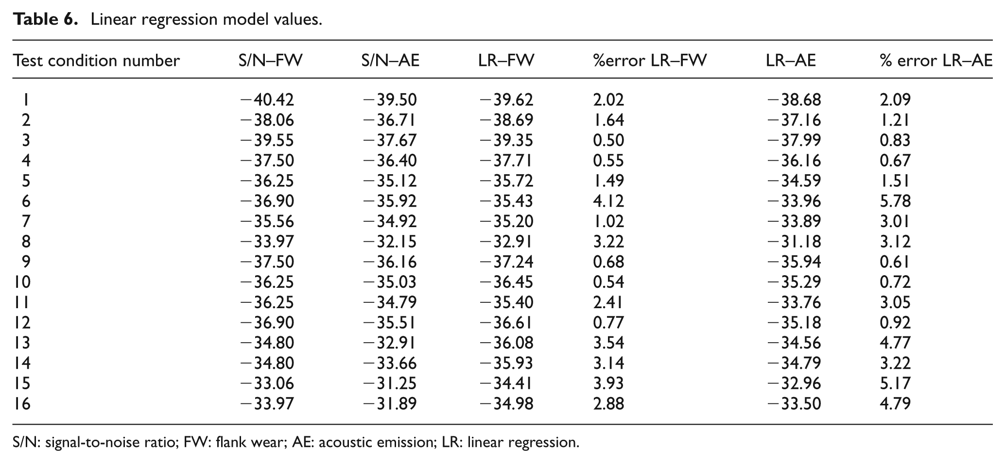
S/N: signal-to-noise ratio; FW: flank wear; AE: acoustic emission; LR: linear regression.

Empirical equation for the audible AE signal based on linear regression model is developed as

$$\text{A}{\text{E}}_{\text{LR}}=-35.2671-(0.0546\times \text{H})+(0.025891\times \text{V})-(5.97837\times \text{f})+(2.94064\times \text{d})$$

(4)

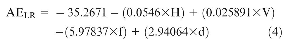
The comparison of S/N ratio values of audible AE with linear regression model values is shown in Figure 4. For verifying the validated results of audible AE signals based on a non-linear regression model, the estimated mean of audible AE was calculated as AE_em = –30.1205. The non-linear regression data for audible AE was developed by using regression analysis as shown in Table 7.

Figure 4.

Comparison of the S/N ratio of AE with linear regression model values.

Table 7.

Summary output – non-linear regression – acoustic emission

	df	SS	MS	F	Significance F
Regression	10	69.44	6.94	10.49	0.009
Residual	5	3.31	0.66
Total	15	72.75
	Coefficient	Standard error	t stat	p-value
Intercept	−38.24	8.27	−4.62	0.005
H	−0.104	0.048	−2.17	0.081
V	0.12	0.053	2.29	0.07
f	−79.23	57.74	−1.37	0.228
d	14.65	15.33	0.95	0.38
(H*V)	−5.7E-05	0.0003	−0.19	0.855
(H*f)	0.525	0.197	2.65	0.045
(H*d)	−0.032	0.041	−0.77	0.473
(V*f)	−0.070	0.311	−0.226	0.829
(V*d)	−0.179	0.077	−2.30	0.069
(f*d)	111.75	53.52	2.087	0.091

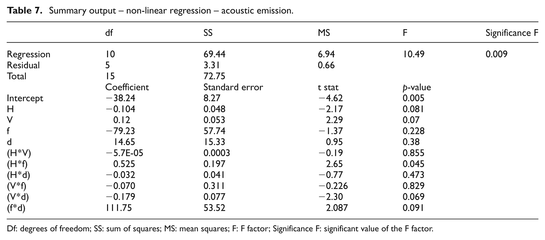
Df: degrees of freedom; SS: sum of squares; MS: mean squares; F: F factor; Significance F: significant value of the F factor.

A confidence interval of 95% for the prediction of audible AE based on the validation experiment on the basis of a non-linear regression model was calculated as

$$\mathrm{CI}=\sqrt{F_{0.05}(3,f_e)V_e[\frac{1}{n}+\frac{1}{R}]}$$

(5)

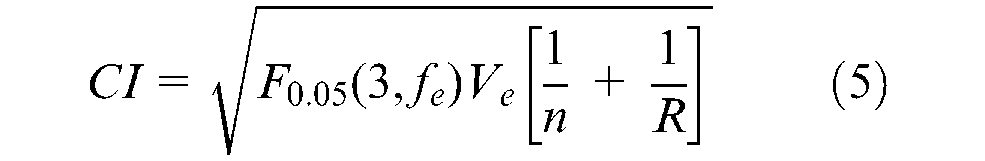
where f_e is the error degrees of freedom (5) from Table 7, F_0.05 (3, f_e) is the F ratio required for risk (3, 5) which equals 9.01 from standard “F” table, ³⁸ V_e is the error variance (0.66) from Table 7, R is the number of repetitions for validation experiment (1), and N is the total number of experiments (16). Where n_r is the number of replications (1), n is the effective number of replications which equals = N/(1 + degrees of freedom associated with audible AE) = 16/(1 + 15) = 1. By substituting the above values in equation (5), the value of the confidence interval (CI) for audible AE based on a non-linear regression model was calculated as

$$\text{CI}={\{9.01\times 0.66[(1/1)+(1/1)]\}}^{1/2}=3.44865$$

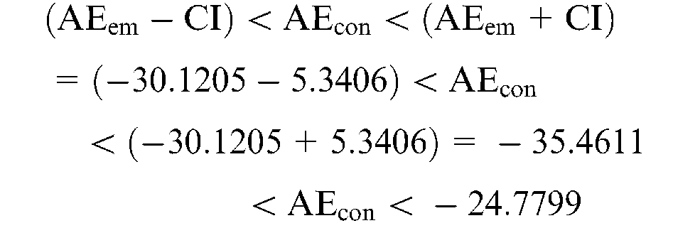
The 95% confidence interval for the optimal audible AE in validation experiment was verified as

$$(\text{A}{\text{E}}_{\text{em}}-\text{CI})<\text{A}{\text{E}}_{\text{con}}<(\text{A}{\text{E}}_{\text{em}}+\text{CI})=(-30.1205-3.44865)<\text{A}{\text{E}}_{\text{con}}<(-30.1205+3.44865)=34.3986<\text{A}{\text{E}}_{\text{con}}<39.4830$$

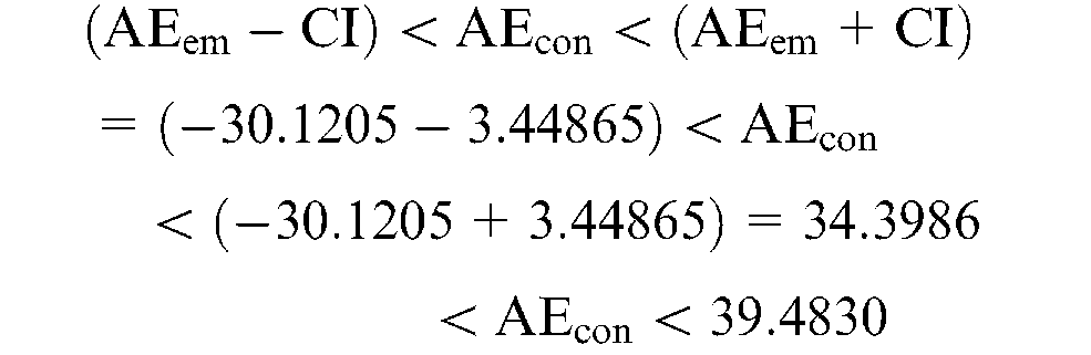
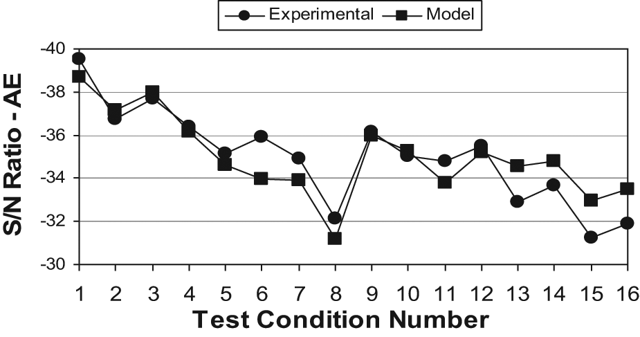
The result of validation experiment shows that the audible AE is −31.2506, which is between −33.56915 and −26.67185. The validated audible AE is thus confirmed by the above calculations. The non-linear regression model values are shown in Table 8. The comparison of the S/N ratio values of audible AE with the non-linear regression model values is shown in Figure 5. The empirical equation for the audible AE signal based on non-linear regression model was developed as

$$\text{A}{\text{E}}_{\text{NLR}}=(-38.24-(0.104\times \text{H})+(0.1219\times \text{V})-(79.237\times \text{f})+(14.656\times \text{d})-(0.00005\times \text{H}\times \text{V})+(0.525\times \text{H}\times \text{f})-(0.032\times \text{H}\times \text{d})-(0.0707\times \text{V}\times \text{f})-(0.1799\times \text{V}\times \text{d})+(111.758\times \text{f}\times \text{d}))$$

(6)

Table 8.

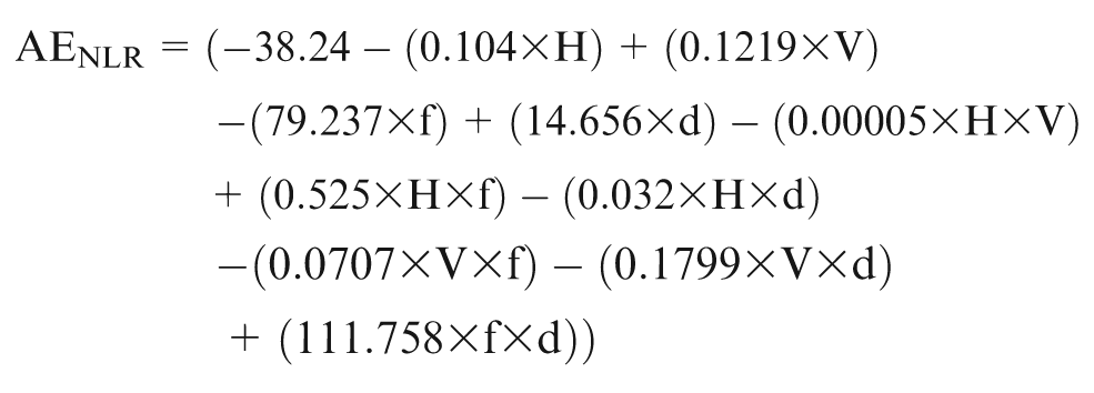
Non-linear regression model values.

Test condition number	S/N–FW	S/N–AE	NLR–FW	%error NLR–FW	NLR–AE	% error NLR–AE
1	−40.42	−39.50	−40.62	0.48	−39.73	0.58
2	−38.06	−36.71	−38.01	0.11	−36.59	0.31
3	−39.55	−37.67	−39.42	0.32	−37.51	0.43
4	−37.50	−36.40	−37.58	0.21	−36.56	0.43
5	−36.25	−35.12	−36.34	0.23	−35.35	0.66
6	−36.90	−35.92	−36.62	0.76	−35.49	1.22
7	−35.56	−34.92	−35.16	1.12	−34.29	1.81
8	−33.97	−32.15	−33.84	0.40	−31.99	0.51
9	−37.50	−36.16	−37.58	0.23	−36.50	0.92
10	−36.25	−35.03	−35.31	2.66	−33.82	3.57
11	−36.25	−34.79	−36.31	0.16	−34.82	0.07
12	−36.90	−35.51	−36.98	0.23	−35.50	0.03
13	−34.80	−32.91	−34.91	0.31	−33.00	0.27
14	−34.80	−33.66	−35.39	1.66	−34.27	1.77
15	−33.06	−31.25	−33.43	1.10	−31.62	1.16
16	−33.97	−31.89	−34.23	0.74	−32.55	2.03

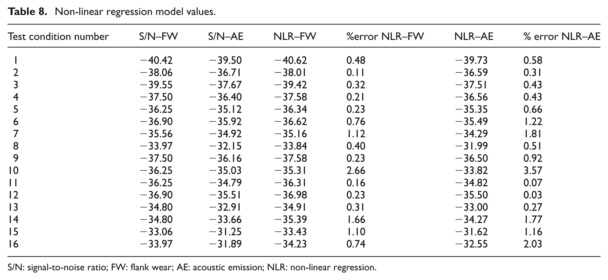
S/N: signal-to-noise ratio; FW: flank wear; AE: acoustic emission; NLR: non-linear regression.

Figure 5.

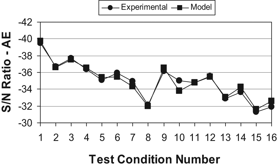
Comparison of S/N ratio of AE with non-linear regression model values.

By substituting the corresponding values of parameters corresponding to test condition number 5 in equations (4) and (6), the predicted values of the S/N ratio audible AE signal were obtained as

$$\text{A}{\text{E}}_{\text{LR}}=-34.5988$$

$$\text{A}{\text{E}}_{\text{NLR}}=-35.3565$$

The experimental value of the audible AE corresponding to the same test condition number 5 is −35.1221. The percentage deviation between the values of experimental audible AE and predicted AE were calculated as

$$\left[\frac{\mathrm{Empiricalvalue}-\mathrm{Experimentalvalue}}{\mathrm{Empiricalvalue}}\right]\times 100$$

$$\%\text{A}{\text{E}}_{\text{LR}}=1.512\%$$

$$\%\text{A}{\text{E}}_{\text{NLR}}=0.6632\%$$

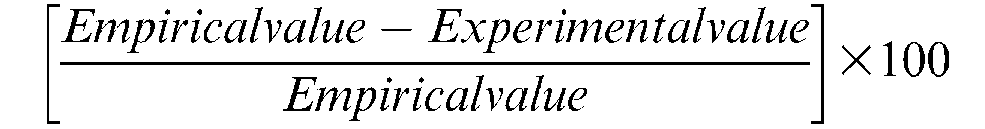
Figure 6 shows the comparison between the percentage error of audible AE in the linear regression model with the percentage error of audible AE in the non-linear regression model.

Figure 6.

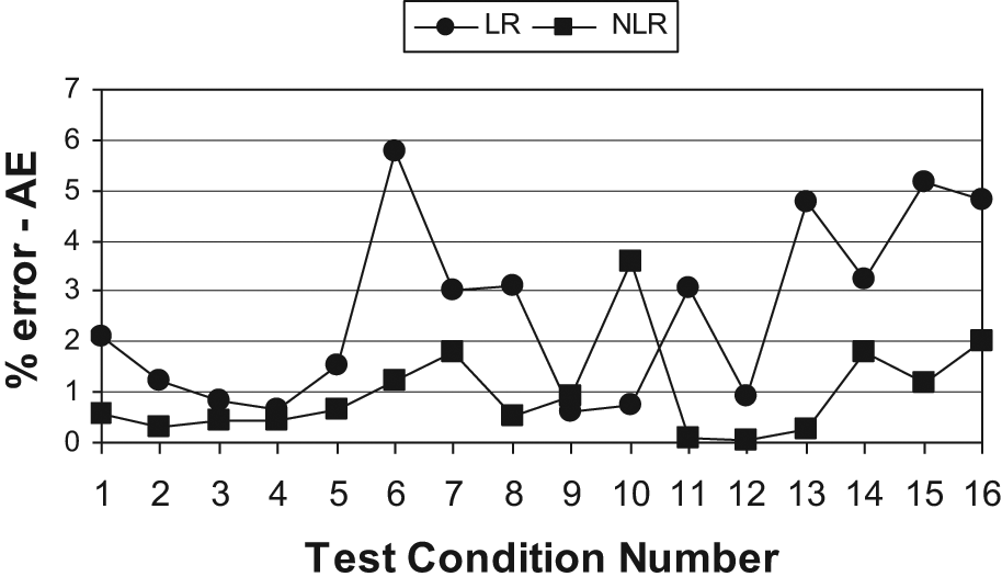
Comparison of the percentage error of linear regression AE and the percentage error of non-linear regression AE.

Since the traditional optimization technique Taguchi’s DoE identifies only the nearest levels of parameters, it is necessary to go for some of the non-traditional optimization techniques. There are several non-traditional optimization techniques, such as the adaptive genetic algorithm, SAA, memetic algorithm, ant colony algorithm, etc., in practice. Even though the SAA shows more or less the same agreement with other optimization techniques, it is comparatively less time consuming for convergence. Hence, it was further decided to use this technique both for linear regression and non-linear regression in order to minimize the audible AE signal and FW by maintaining the value of surface roughness (constraint) well below 5.00 microns.

In the SAA, the initial temperature (T) and decrement factor (d) are the two important parameters that govern the successful working of the simulated annealing procedure. If a larger initial value of ‘T’ (or ‘d’) is chosen, it takes more iterations for convergence. On the other hand, if a small value of the initial temperature ‘T’ is chosen, the search is not adequate to thoroughly investigate the search space before converging to the true optimum. Unfortunately, there are no unique values of the initial temperature (T), decrement factor (d) and number of iterations (n) that work for every problem. However, an estimate of the initial temperature can be obtained by calculating the average of the function values at a number of random points in the search space. A suitable value of ‘n’ can be chosen (usually between 2 and 100) depending on the available computing resource and the solution time. The decrement factor is left to the choice of the user. However, the initial temperature and subsequent cooling schedule require some trial and error efforts. Hence, different combinations of these two parameters were analyzed and the best results were obtained for the following combinations, both for linear and non-linear equations. There were better results for different possible combinations of these two parameters. All the possible combinations were tried out for linear equation and are shown below.

Number of iterations, n = 200 (convergence occurs at iteration number 79)

$$\text{T}=1{00}^{\circ }\text{C},\text{df}=0.1\text{and COF}=0.62404$$

$$\text{T}=1{00}^{\circ }\text{C},\text{df}=0.2\text{and COF}=0.624$$

$$\text{T}=1{00}^{\circ }\text{C},\text{df}=0.3\text{and COF}=0.62399$$

$$\text{T}=1{00}^{\circ }\text{C},\text{df}=0.4\text{and COF}=0.62399$$

$$\text{T}=1{00}^{\circ }\text{C},\text{df}=0.5\text{and COF}=0.62388$$

$$\text{T}=1{00}^{\circ }\text{C},\text{df}=0.6\text{and COF}=0.62391$$

$$\text{T}=1{00}^{\circ }\text{C},\text{df}=0.7\text{and COF}=0.62404$$

$$\text{T}=1{00}^{\circ }\text{C},\text{df}=0.8\text{and COF}=0.62387$$

$$\text{T}=1{00}^{\circ }\text{C},\text{df}=0.9\text{and COF}=0.62387$$

$$\text{T}=1{000}^{\circ }\text{C},\text{df}=0.9\text{and COF}=0.62398$$

From the various combinations, with the temperature and decrement factor values maintained at 100 °C and 0.8, the minimum value of combined objective function (COF) (0.62387) was obtained. When the temperature and decrement factor values were selected as 100 °C and 0.9, the same value of COF was obtained, but the number of iterations is increased to 141. Hence, these temperature and decrement factor values were not considered in this study. The temperature of 1000 °C does not improve the value of COF and hence, this temperature was also not considered in this analysis. The best levels of parameters obtained using the SAA based on the linear regression equation, and the corresponding S/N values of audible AE and surface roughness are presented in Figure 7.

Figure 7.

Output of the SAA for AE based on linear regression.

The better results for different possible combinations of initial temperature and decrement factor were also tried out for non-linear equation. It is found that, when the temperature and decrement factor were maintained at 100 °C and 0.4, the minimum value of COF (0.51715) was obtained, which is less than all the values obtained from the linear regression equation. The best levels of parameters obtained using the SAA based on the non-linear regression equation, and the corresponding S/N values of audible AE and surface roughness, are presented in Figure 8. The comparison of output of the SAA for linear regression and non-linear regression based on audible AE is shown in Figure 9.

Figure 8.

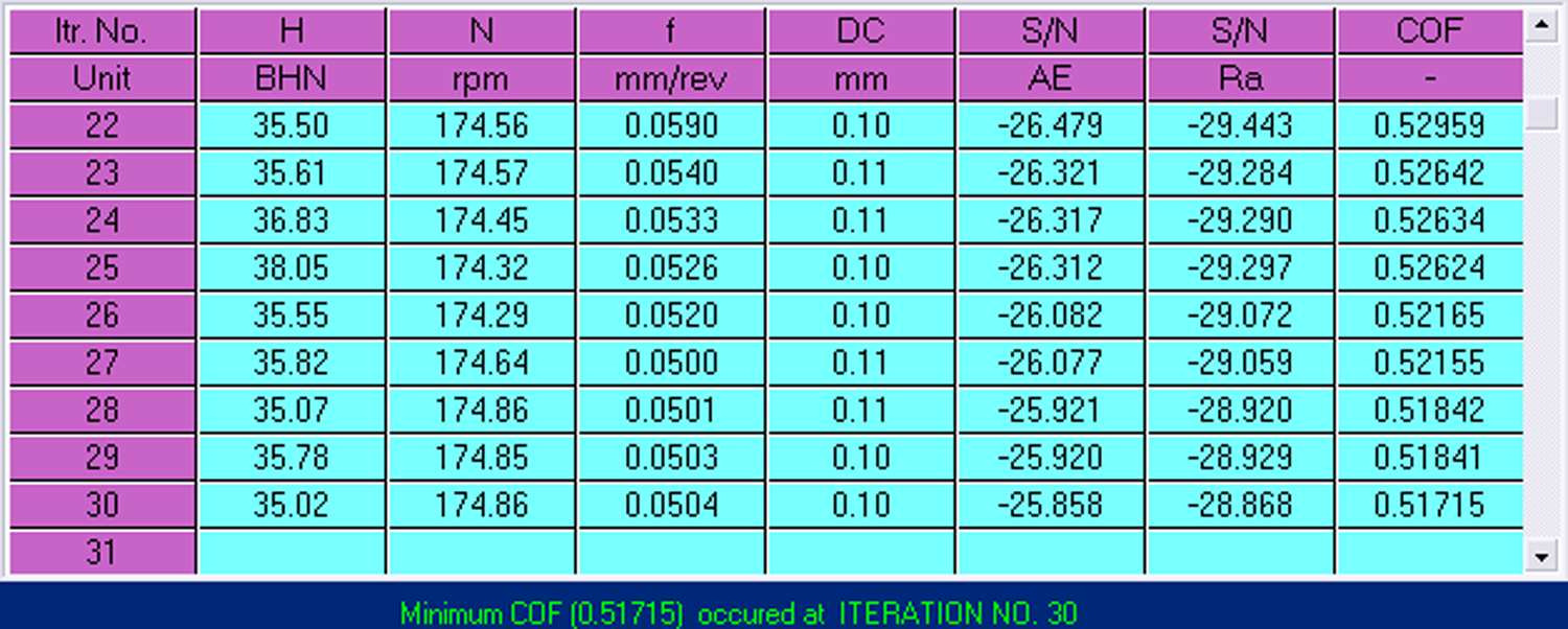
Output of the SAA for AE based on non-linear regression.

Figure 9.

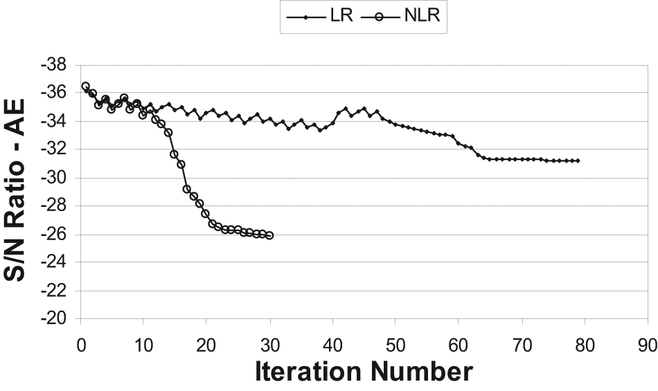
Comparison of output of the SAA for linear and non-linear regression based on AE.

For verifying the validated results of FW with the linear regression model, the estimated mean of FW was calculated and determined as

$$\text{F}{\text{W}}_{\text{em}}=-32.3714$$

The linear regression data for FW was developed by using regression analysis as shown in Table 9. A confidence interval of 95% for the prediction of FW based on the validation experiment on the basis of the linear regression model was obtained as

$$\text{CI}=4.2767$$

Table 9.

Summary output – linear regression – flank wear.

	df	SS	MS	F	Significance F
Regression	4	49.00	12.25	11.72	0.000588
Residual	11	11.490	1.044
Total	15	60.491
	Coefficient.	Standard error	t stat	p-value
Intercept	−35.74	1.57	−22.70	1.37E-10
H	−0.053	0.008	−6.049	8.31E-05
V	0.021	0.0091	2.349	0.0385
f	−6.80	4.570	−1.487	0.1649
d	2.137	1.330	1.606	0.1365

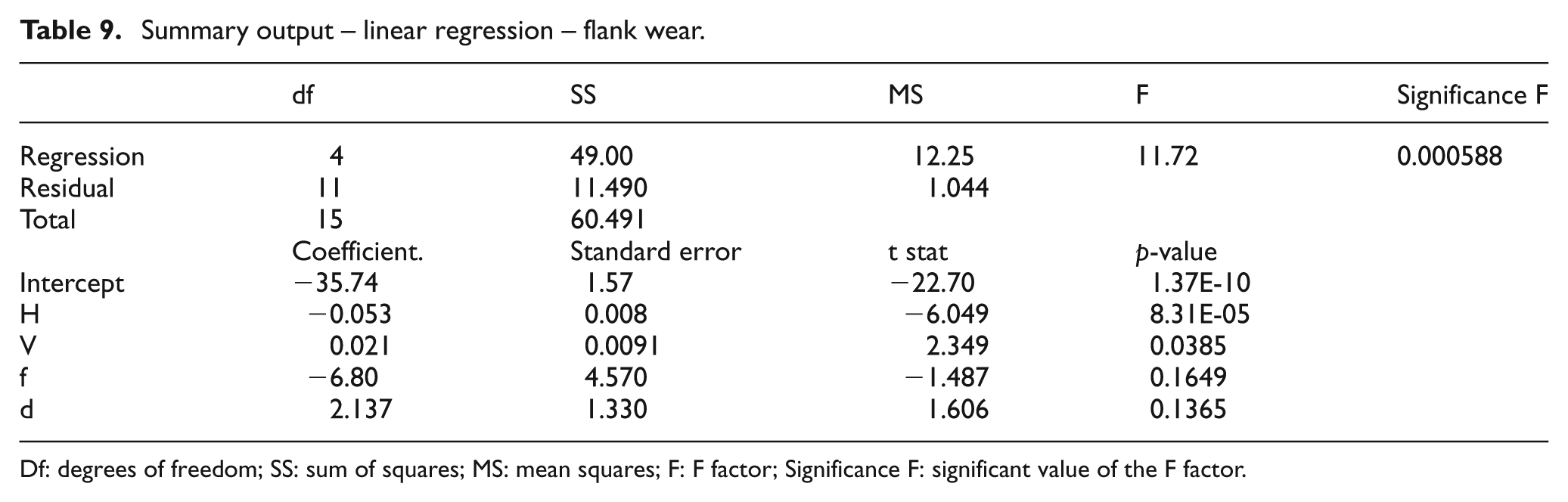
Df: degrees of freedom; SS: sum of squares; MS: mean squares; F: F factor; Significance F: significant value of the F factor.

The 95% confidence interval for the optimal FW in validation experiment was verified as

$$(\text{F}{\text{W}}_{\text{em}}-\text{CI})<\text{F}{\text{W}}_{\text{con}}<(\text{F}{\text{W}}_{\text{em}}+\text{CI})=(-32.3714-4.2767)<\text{F}{\text{W}}_{\text{con}}<(-32.3714+4.2767)=-36.6481<\text{F}{\text{W}}_{\text{con}}<-28.0947$$

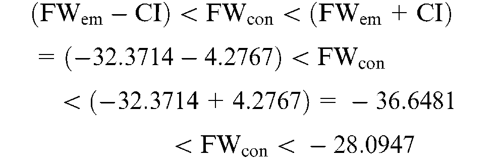
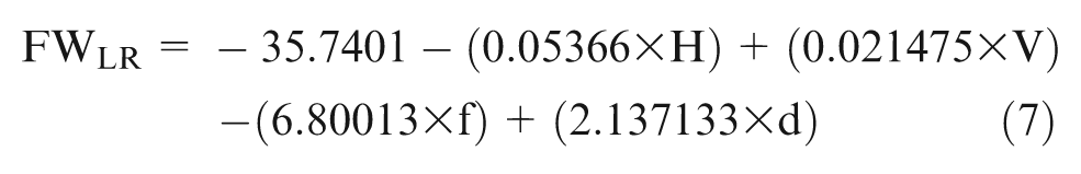
The result of the validation experiment shows that the FW is −33.4546, which is between −36.6481 and −28.0947. The validated FW was thus confirmed by the above calculations. The linear regression model values are shown in Table 5. The comparison of the S/N ratio values of FW with the linear regression model values is shown in Figure 10. Empirical equation for the FW based on the linear regression model was developed as

$$\text{F}{\text{W}}_{\text{LR}}=-35.7401-(0.05366\times \text{H})+(0.021475\times \text{V})-(6.80013\times \text{f})+(2.137133\times \text{d})$$

(7)

Figure 10.

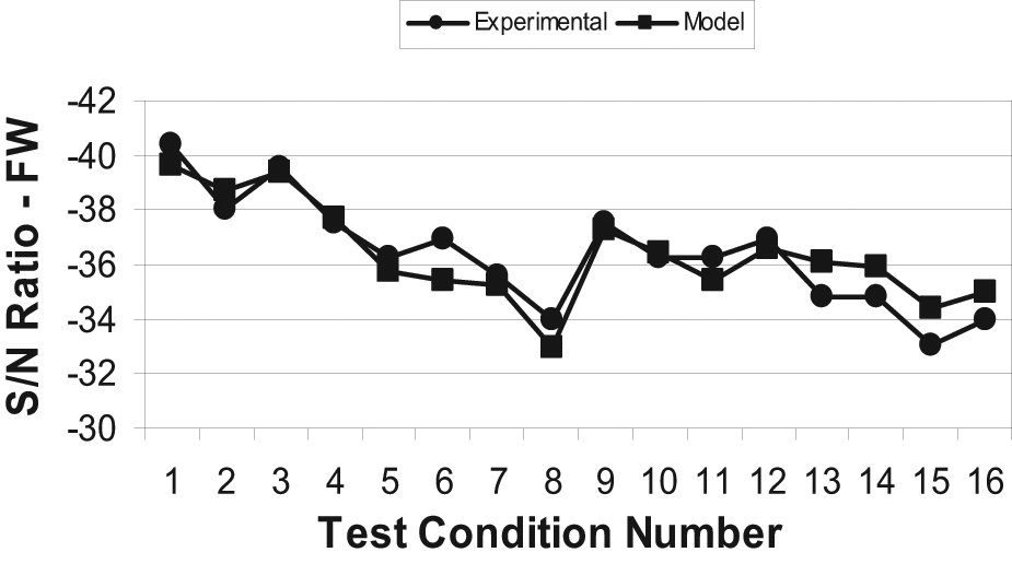
Comparison of the S/N ratio of FW with linear regression model values.

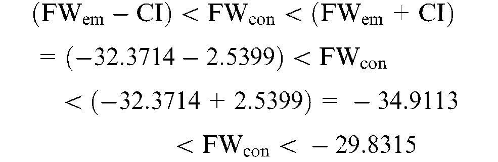
For verifying the validated results of FW with the non-linear regression model, the estimated mean of FW was calculated as FW_em = –32.3714. The non-linear regression data for FW was developed by using regression analysis as shown in Table 10. A confidence interval of 95% for the prediction of the mean FW based on the validation experiment on the basis of the non-linear regression model was calculated as CI = 2.5399. The 95% confidence interval of the optimal FW in the validation experiment was verified as

$$(\text{F}{\text{W}}_{\text{em}}-\text{CI})<\text{F}{\text{W}}_{\text{con}}<(\text{F}{\text{W}}_{\text{em}}+\text{CI})=(-32.3714-2.5399)<\text{F}{\text{W}}_{\text{con}}<(-32.3714+2.5399)=-34.9113<\text{F}{\text{W}}_{\text{con}}<-29.8315$$

Table 10.

Summary output – non-linear regression – flank wear.

	df	SS	MS	F	Significance F
Regression	10	58.69	5.86	16.37	0.003257
Residual	5	1.792	0.358
Total	15	60.49
	Coefficient	Standard error	t stat	p-value
Intercept	−40.51	6.08	−6.65	0.001
H	−0.09	0.035	−2.57	0.049
V	0.112	0.039	2.869	0.035
f	−38.68	42.49	−0.910	0.404
d	10.81	11.2	0.957	0.382
(H*V)	−2.4E-05	0.0002	−0.107	0.918
(H*f)	0.308	0.145	2.122	0.087
(H*d)	0.0088	0.0305	0.28	0.784
(V*f)	−0.180	0.229	−0.78	0.466
(V*d)	−0.149	0.057	−2.60	0.047
(f*d)	78.19	39.390	1.985	0.103

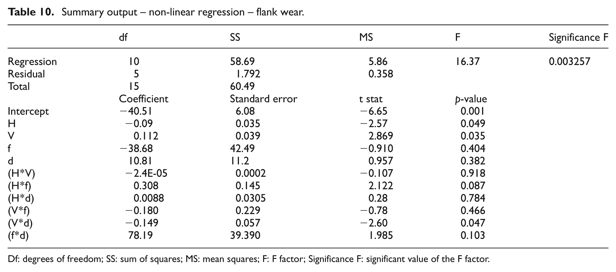
Df: degrees of freedom; SS: sum of squares; MS: mean squares; F: F factor; Significance F: significant value of the F factor.

The result of validation experiment shows that the FW is −33.4546, which is between −34.9113 and −29.8315. The validated FW was thus confirmed by the above calculations. The non-linear regression model values are shown in Table 7. The comparison of S/N ratio values of FW with the non-linear regression model values is shown in Figure 11.

Figure 11.

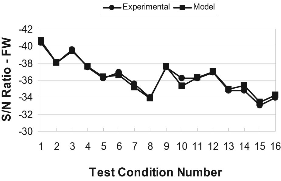
Comparison of the S/N ratio of FW with non-linear regression model.

The empirical equation for the FW based on the non-linear regression model was developed as

$$\text{F}{\text{W}}_{\text{NLR}}=(-40.5191-(0.0911\times \text{H})+(0.1124\times \text{V})-(38.6814\times \text{f})+(10.8134\times \text{d})-(0.000024\times \text{H}\times \text{V})+(0.0.3089\times \text{H}\times \text{f})+(0.0088\times \text{H}\times \text{d})-(0.1806\text{V}\times \text{f})-(0.14966\times \text{V}\times \text{d})+(78.1911\times \text{f}\times \text{d}))$$

(8)

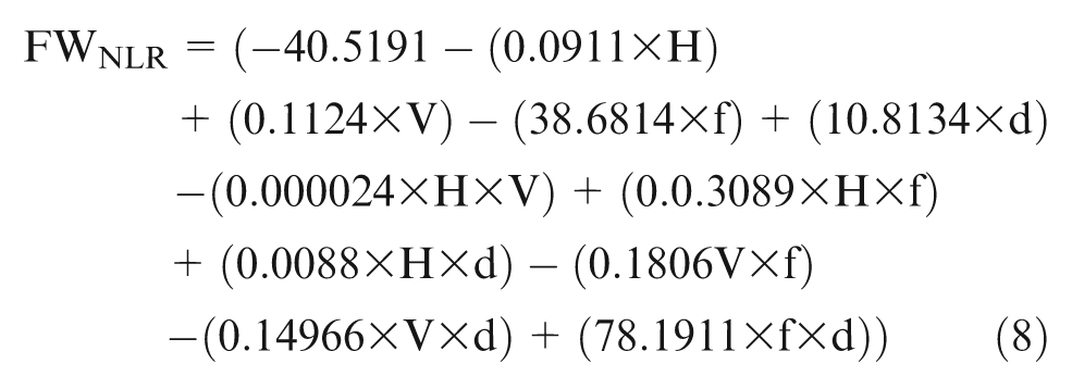
By substituting the corresponding values of parameters corresponding to test condition number 5 in equations (7) and (8), the predicted values of FW were obtained as

$$\text{F}{\text{W}}_{\text{LR}}=-35.7235$$

$$\text{F}{\text{W}}_{\text{NLR}}=-36.3428$$

An experimental value of FW corresponding to the same test condition number 5 is −36.2583. The percentage deviation between the values of experimental FW and predicted FW were calculated and found as

$$\%\text{F}{\text{W}}_{\text{LR}}=1.497\%$$

$$\%\text{F}{\text{W}}_{\text{NLR}}=0.2326\%$$

Figure 12 shows the comparison between percentage error of FW in the linear regression model with percentage error of FW in the non-linear regression model.

Figure 12.

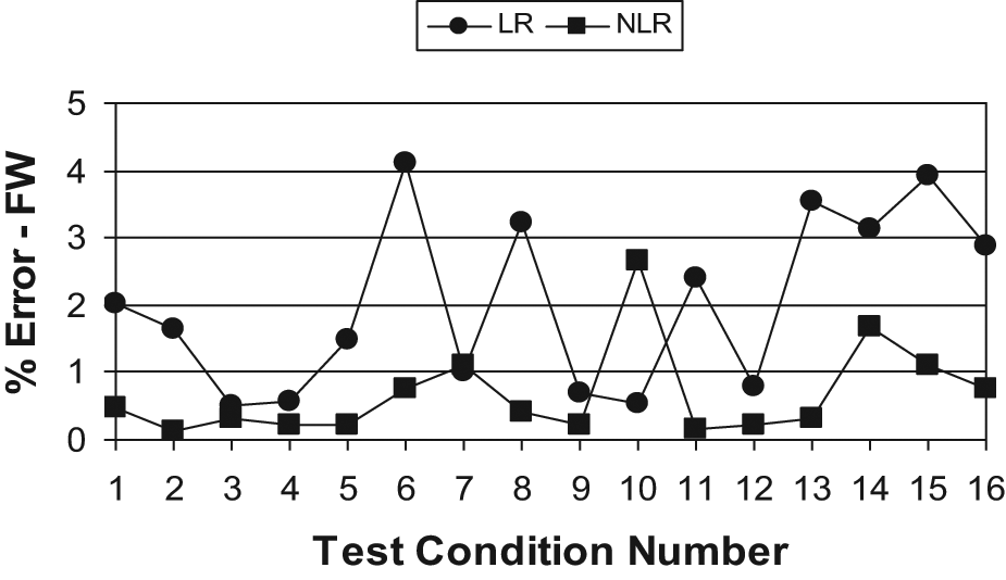
Comparison of percentage error of linear regression flank wear and percentage error of non-linear regression flank wear.

The better results for different possible combinations of initial temperature and decrement factor were also tried out for the linear and non-linear equation for FW using the SAA. It was found that, when the temperature and decrement factor are maintained at 1000 °C and 0.9, the minimum value of COF (0.65855) was obtained using the linear regression equation. The best levels of selected parameters obtained using the SAA for the linear regression equation and the S/N values of FW and surface roughness are presented in Figure 13. It was also found that, when the temperature and decrement factor are maintained at 200 °C and 0.1, the minimum value of COF (0.56614) is obtained using the non-linear regression equation, which is less than all the better values obtained from the linear regression equations. The best levels of selected parameters obtained using the SAA for the non-linear regression equation, and the S/N values of audible AE and surface roughness, are presented in Figure 14. The comparison of output of SAA for linear regression and non-linear regression based on FW is shown in Figure 15. The comparison of the S/N ratio values of FW and S/N ratio of audible AE signal value are shown in Figure 16.

Figure 13.

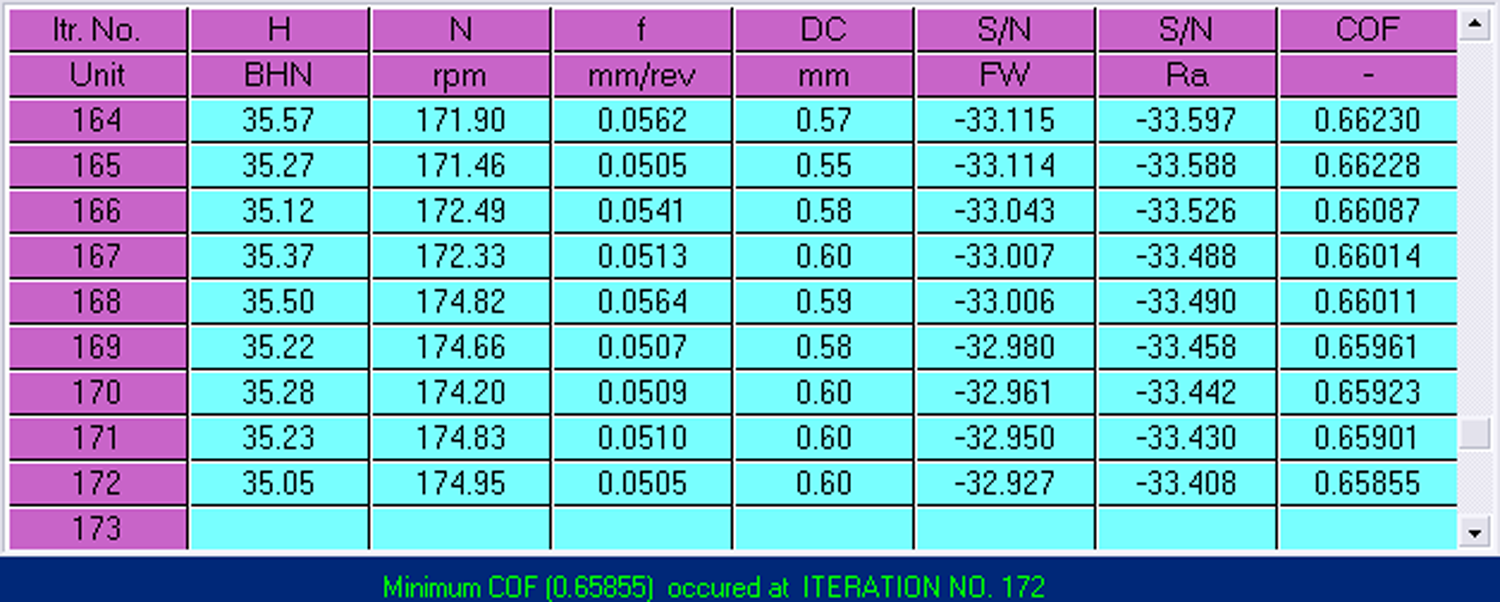
Output of the SAA for FW based on linear regression.

Figure 14.

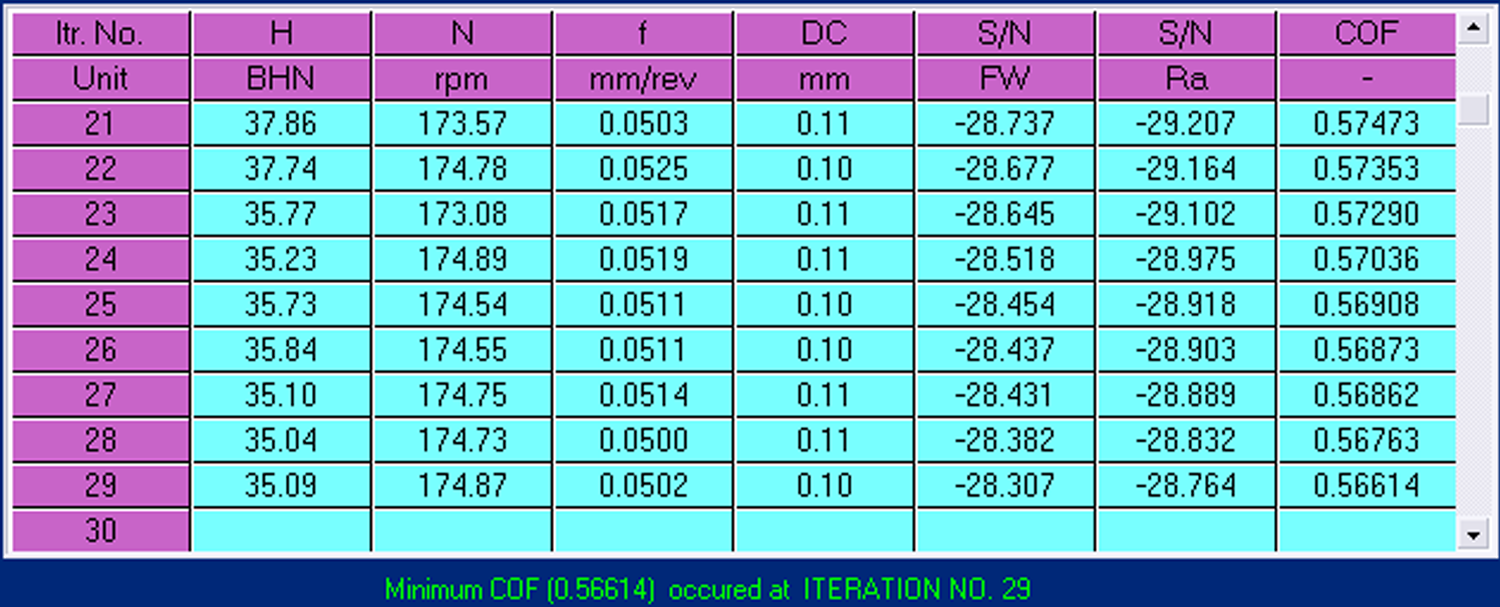
Output of the SAA for AE based on non-linear regression.

Figure 15.

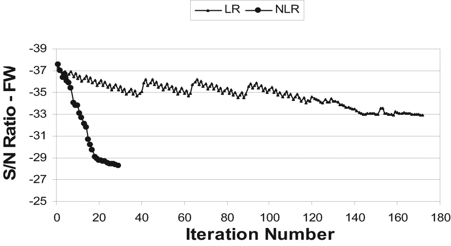
Comparison of output of the SAA for linear regression and non-linear regression based on FW.

Figure 16.

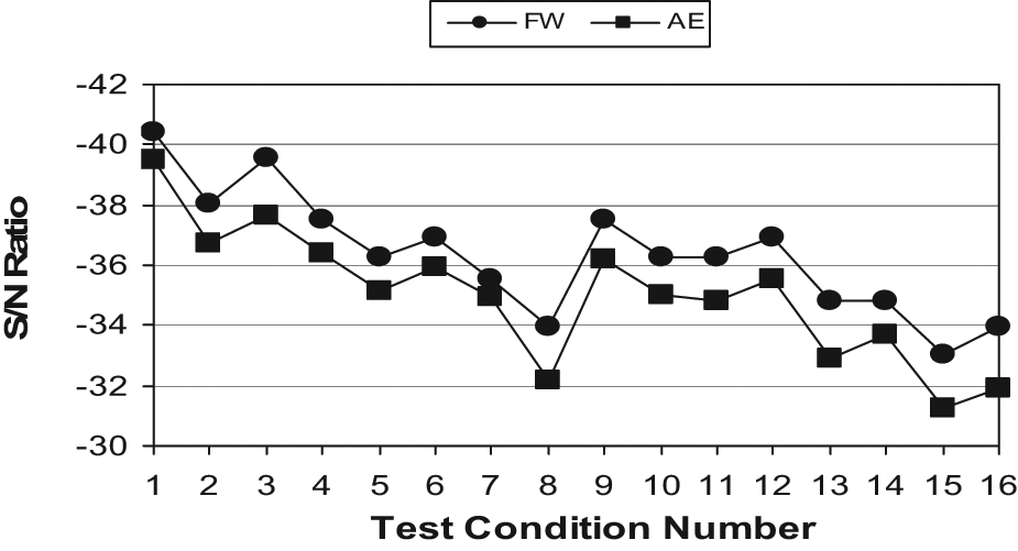
Comparison of the S/N ratio of FW and S/N ratio of AE.

Finally, the comparison of FW structure captured by a scanning electron microscope for the two different levels of hardness (110 BHN and 35 BHN) of a workpiece is shown in Figure 17(a) and (b).

Figure 17.

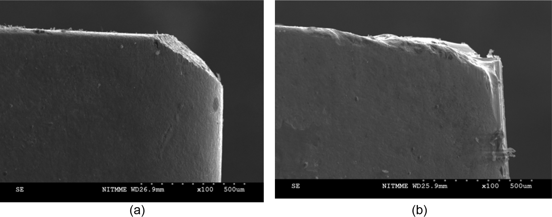
Comparison of FW structure of the cutting insert for two different levels (110 BHN and 35 BHN) of hardness values of workpieces.

Conclusions

In this article, the audible AE signal developed during turning used for monitoring the FW online basis is explained. Based on the experimentation and analysis, the following conclusions are drawn:

1. By using Taguchi’s DoE, the optimal levels of parameters are obtained and the validation experiment was conducted. The minimum value of FW obtained in the validation experiment is 45 µm, which is lower than that of all the tabulated experimental values by at least 10%.

2. In Figures 4 and 10, the trend between experimental S/N–AE and S/N–FW is uniform with a good correlation of linear predicted values of audible AE and FW. From the correlation between the trends of experimental audible AE and FW with predicted values of audible AE and FW, it is concluded that it is possible to use this developed model for the prediction of the objectives for all test conditions.

3. Also, as the trend between experimental S/N–AE and S/N–FW is almost the same as the predicted values of audible AE and FW using the non-linear regression model in Figures 5 and 11, the predicted model using the non-linear regression model can feasibly be used for the prediction of audible AE and FW for all test conditions of any range of selection.

4. From Figures 6 and 12, it is well defined that the non-linear regression model shows a comparatively minimum deviation of audible AE and FW when compared with the linear regression model for all test conditions.

5. Figures 9 and 15 show that the non-traditional optimization technique using the non-linear regression model gives a comparatively better combination of parameters to obtain minimum FW and audible AE when compared with the linear regression model.

6. Figure 16 shows a very close relationship between S/N–AE and S/N–FW. From this, it is concluded that, it is possible to use the online observation of the audible AE signal during machining as an indirect technique for monitoring the FW of the cutting insert with reference to their acceptable linear trend.