Experimental and numerical investigation of an adaptive simulated annealing technique in optimization of warm tube hydroforming

Abstract

Simulated annealing technique – which has attracted significant attention as being suitable for combinatorial optimization problems – has been used in many engineering applications. In current research, this method is used in optimization of a complicated forming process. Warm tube hydroforming is a new technology in the forming of lightweight aluminum and magnesium alloys in automotive, electronics and leisure industries. Owing to the complex nature of this process at high temperatures, and difficulty of obtaining the optimized forming conditions, this process has not received the credit it deserves yet. A new method for optimization of the warm tube hydroforming process is developed by using the simulated annealing algorithm with a novel adaptive annealing schedule. The optimal pressure loading paths are obtained for AA6061 aluminum alloy tubes with different wall thicknesses and corner fillets. The results obtained by simulated annealing technique are verified numerically and experimentally.

Introduction

Product quality, energy efficiency, time and cost are considered the most important research topics in manufacturing industries these days. Optimization is an effective way to gain this aim. Many optimization techniques are proposed for different kinds of problems, and many researches have been dedicated to finding the best ways to obtain the optimum results for various processes. Practical problems are in different fields, such as management, computer science and engineering. Solving an optimization problem is to find an optimal or near-optimal response out of a finite number of solutions.

Simulated annealing (SA) is a very efficient technique in combinatorial optimization problems. SA is a generic probabilistic metaheuristic, derived by a natural analogy with the statistical physics of random systems. Heuristic methods are used to find good solutions with acceptable computational time and cost. From the metallurgical point of view, SA is the simulation of a heated metal being cooled. During an annealing process, the metal is assumed to be at its highly ordered, minimum energy state. Therefore, the temperature has to be gradually decreased so that the material is in equilibrium at each temperature, and the crystalline structure of metal has formed homogeneously with the minimal energy level. The idea of using SA for optimization problems was first proposed by Kirkpatrick et al. ¹ based on the Metropolis algorithm, a Monte Carlo method that is a class of computational algorithms that relies on repeated random sampling to compute their results. Application of SA is widely increased in optimization of engineering problems, but to the best knowledge of the authors, it is not widely used in forming processes. Finding the optimal definitions for SA parameters is totally problem dependent on an empirical basis. Many researchers have tried to develop adaptive definitions for these parameters, such as annealing schedule, Markov chain length (MCL) and convergence condition. Lin et al. ² developed an algorithm with a combination of SA and genetic algorithm (GA), and tried to select the MCL adaptively according to the population size. Sohn, ³ Wong and Constantinides, ⁴ Pao et al., ⁵ Thompson and Bilbro ⁶ and Wu and Chow ⁷ selected the number of inner loops as a constant but problem dependent. Xavier-de-Souza et al. ⁸ decided the temperature reduction time when thermal equilibrium is reached at each temperature. Atiqullah and Rao ⁹ implemented the SA algorithm by augmenting it with a feasibility improvement scheme to formulate and solve a two part stamping optimization problem without artificially modifying the objective function.

The aim of this article is to develop a new concept of the SA technique with an adaptive annealing schedule in optimization of a metal-forming process known as warm tube hydroforming (WTH). A simple case with simple geometry and forming conditions is selected at this stage of the research to validate the approach. The authors believe that this approach has many capabilities and potentials to be used in optimization of complex manufacturing processes along with other intelligent systems, such as GA, neural networks and fuzzy-assisted systems.

Problem statement

Tube hydroforming is a cost-effective way of shaping metal tubes into lightweight, structurally stiff and strong pieces. In the tube hydroforming process, hydraulic pressure (usually oil or water) is applied into a tube inside a die with the desired cavity shape. The tube ends are sealed by axial punches, and the internal pressure is increased up to the designed value by injecting through one of the axial punches. This causes the tube to form against the die cavity surface. Usually axial force is also applied to flow the material into the bulging zone. Figure 1 shows a schematic of this process. The process requires the proper combination of part design, material selection, and application of internal pressure and axial feeding. The automotive industry is the most enthusiastic adopter of the hydroforming process, which makes production of the complex shapes possible by lighter and more rigid integrated structures for vehicles. Owing to the role of weight reduction in fuel consumption, manufacturing of the hydroformed parts out of lightweight materials, such as aluminum and magnesium alloys, has gained many interests in recent years. The main shortcoming of aluminum and magnesium alloys with a high strength-to-weight ratio and good resistance to corrosion is their low toughness and formability at room temperature.^10,11 Their inferior formability is because of the hexagonal closed pack structure in magnesium alloys, and high alloy percentages in aluminum alloys, which reduce the number of slip planes. A solution to enhance the formability of these materials is forming at elevated temperatures, usually below the recrystallization temperature. ¹² At this temperature, additional sliding planes are activated. Application of the hydroforming process at high temperatures for the manufacturing of aluminum and magnesium alloy products makes it possible to achieve the benefits of both methods.

Figure 1.

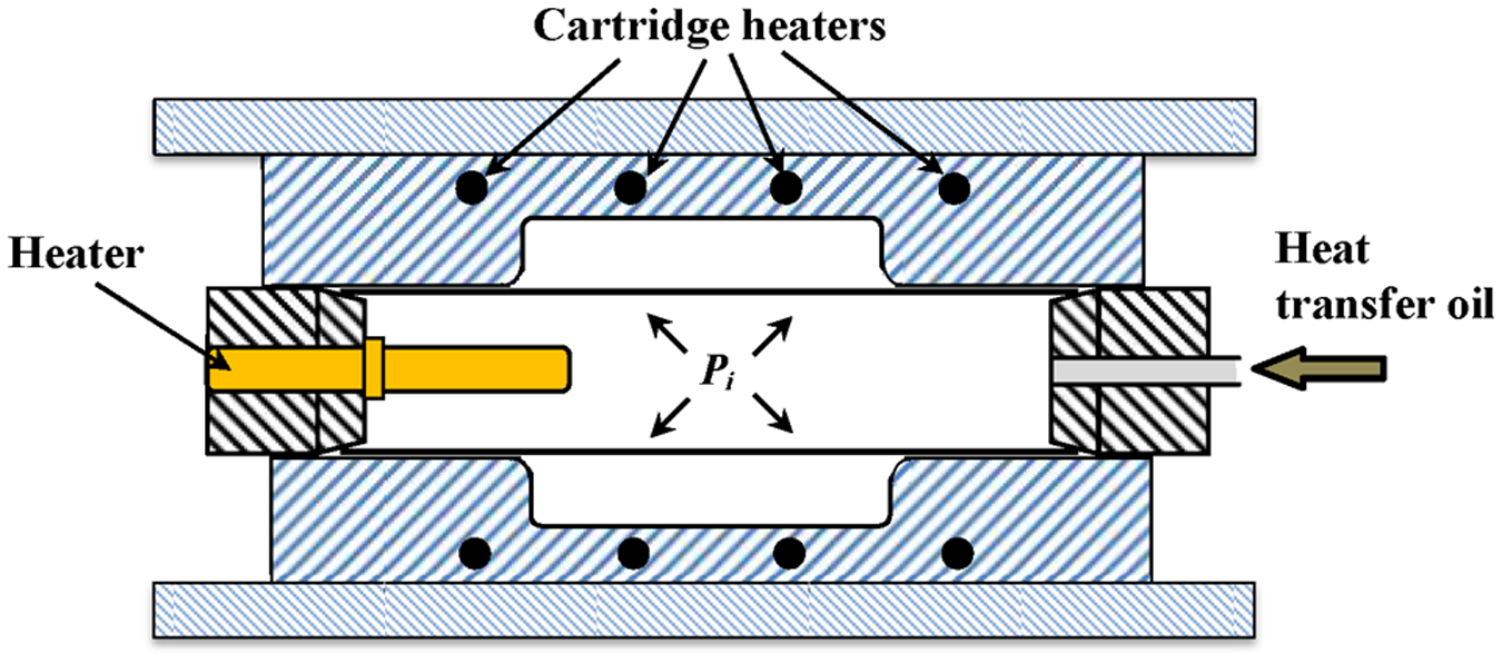
Schematic of WTH.

Proper prediction and control of WTH parameters, especially temperature, pressure and feed loading paths, are key factors in process success. But it is hard to determine the appropriate processing parameters of WTH because of the complicated deformation nature of aluminum alloys at high temperatures. Traditionally, the pressure loading path is obtained by simple theoretical equations, and then improved by finite element (FE) simulations. However, different optimization methods have also been proposed by researchers to improve loading conditions in the tube hydroforming process, but not at warm conditions. A gradient-based optimization method was used in optimization of tube hydroforming.^13,14 A response surface method was used in optimization of the process parameters. ¹⁵ A fuzzy control algorithm was utilized in the loading optimization of tube hydroforming.^16–20 A multi-objective optimization method using FE analysis and the Taguchi method was used in optimization of hydroforming parameters. ²¹ Optimization software, such as LS-OPT ²² and HEEDS ²³ were applied to optimize the loading paths. Neural network, and several optimization methods including hill climbing and SA, were adopted in determination of the loading conditions for T-joints. ²⁴ A hybrid method was utilized to optimize loading paths of tube hydroforming. ²⁵ The MOGA method was applied in multi-objective optimization of multi-stage tube forming. ²⁶ Self-feeding (SF) and adaptive simulation (AS) approaches were used as FE analysis strategies for process design. ²⁷ T-shaped hydroforming was optimized using a SA method. ²⁸ A non-adaptive SA method was proposed and validated by the authors to optimize the hydroforming of copper tubes at room temperature.^29–31

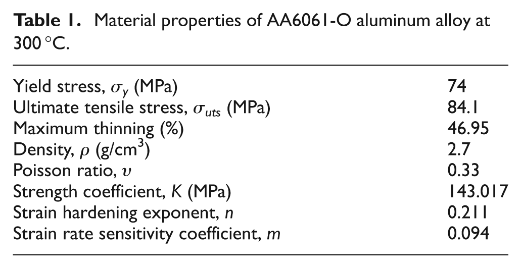
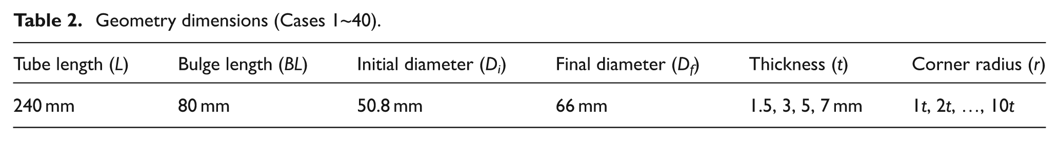
In current research, an adaptive SA algorithm written in MATLAB is linked with a commercial nonlinear finite-element code ANSYS/Ls-Dyna to optimize the pressure loading path in WTH without axial feed. A new adaptive annealing schedule is developed to be used in a SA algorithm and compared with other literature. Methodology is fully explained, and the algorithm is presented as a pseudocode (Appendix 2). Process parameters for hydroforming of the annealed AA6061 aluminum tube shown in Figure 2 have been obtained by the SA method, and verified by experiments. Table 1 shows the material properties from the stress–strain curves obtained by uniaxial tensile tests at 300 °C. The temperature is kept constant during the tests. All dimensions are parametrically defined using ANSYS Parametric Design Language (APDL) to make it easy for the user to select any dimensions. Table 2 shows 40 different cases, which are investigated at 300 °C. The expansion ratio for aluminum alloys is very low at room temperature, but it is selected as 29.92% for this product at 300 °C, which shows a highly improved formability. An optimized pressure loading path is found for each case, and compared with theoretical predictions. The optimal pressure fully forms the final geometry with the minimum thinning and without any defects. Corner fillet and tube thickness, which have great effect on internal pressure, are also discussed. Experiments are then performed using the WTH system for one case to validate the numerical results.

Table 1.

Material properties of AA6061-O aluminum alloy at 300 °C.

Yield stress, σ y (MPa)	74
Ultimate tensile stress, σ uts (MPa)	84.1
Maximum thinning (%)	46.95
Density, ρ (g/cm3)	2.7
Poisson ratio, υ	0.33
Strength coefficient, K (MPa)	143.017
Strain hardening exponent, n	0.211
Strain rate sensitivity coefficient, m	0.094

Table 2.

Geometry dimensions (Cases 1~40).

Tube length (L)	Bulge length (BL)	Initial diameter (D i )	Final diameter (D f )	Thickness (t)	Corner radius (r)
240 mm	80 mm	50.8 mm	66 mm	1.5, 3, 5, 7 mm	1t, 2t, …, 10t

Figure 2.

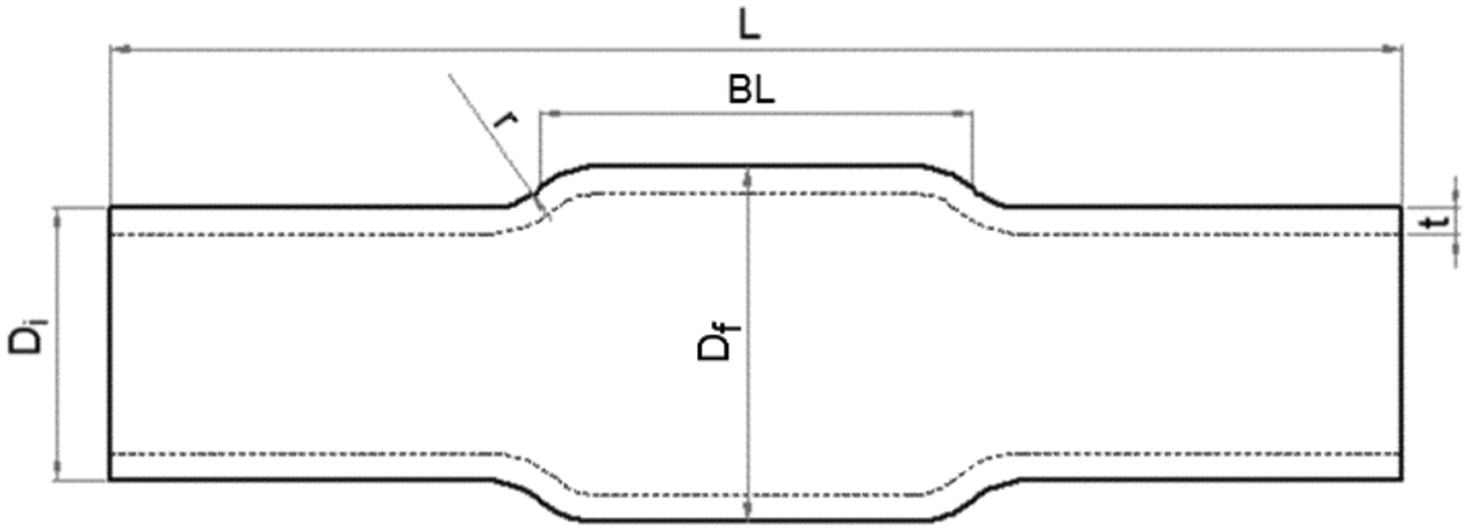
Parametric dimensions of the final tube.

Numerical procedure

The optimization process is a very time-consuming procedure. Two parameters have the highest effect on total time; the number of iterations and FE simulation time. The number of iterations is dependent on the algorithm parameters, while the simulation time is affected by the modeling conditions (type, number and size of the elements, and boundary conditions) and the PC configuration. To reduce the simulation time, a two-dimensional (2D) axisymmetric element PLANE162 is selected in ANSYS/Ls-Dyna. Boundary conditions (BC) in this model are the axial movement constraints on both tube ends, and face load (pressure) on all elements. The effect of the strain rate is not negligible at high temperatures, so the strain rate-dependent plasticity model is used. The material model follows a Ramburgh–Osgood constitutive relationship of the form $\sigma =K{\epsilon }^n{\stackrel{·}{\epsilon }}^m$ . The effect of temperature gradient is not considered owing to simplicity and time. The number and size of the elements are parametrically dependent on the tube length and thickness, which are minimized but still effective. The round of t/1.3 elements in width and 3L elements in length are used in initial tube meshing, i.e. for a 5 mm thickness tube with 240 mm length there will be 2160 elements on the tube. The PC used for simulations is Intel® Core™ i7 CPU 2.8 GHz and 3 GB RAM. It takes 4∼5 min for each simulation. In order to decrease the number of iterations, in addition to proper definition of the annealing schedule, it is very important to narrow the search space as much as possible. So it is required to properly determine the upper and lower bounds for internal pressure. More precise, these estimations are, the sooner the results converge to the optimized one. So, the basic theoretical equations are used to define the upper and lower bounds. “Bursting pressure”– the minimum needed pressure to start the deformation in the tube – is assumed as the lower bound (LB); and “calibration pressure”– the pressure needed to form the sharp corners – as the upper bound (UB). Since these equations are developed for simple geometries, the upper bound is multiplied by a correction coefficient of three for more complex parts. Equations (1) and (2) show the bursting and calibration pressures, respectively ³²

$$P_{\mathrm{bursting}}={\sigma }_{\mathrm{UTS}}\frac{2t}{(D_i-t)}$$

(1)

$$P_{\mathrm{calibration}}=\frac{2}{\sqrt{3}}{\sigma }_f\left[\ln \frac{r}{r-t}\right]$$

(2)

where, ${\sigma }_{\mathrm{UTS}}$ is the ultimate tensile strength of the material, t the tube initial thickness, D _i the tube initial diameter, ${\sigma }_f$ the flow stress of the material and r the smallest die corner radius.

The SA algorithm for the WTH process is summarized in a pseudocode, presented in Appendix 2.

SA method

In an annealing process, a heated metal, disordered at a high temperature, is slowly cooled down so that the system at any time is approximately in thermodynamic equilibrium. At high temperatures, the molecules move freely. As cooling proceeds, the system becomes more ordered and approaches a steady-state. ³³ In the SA method, inspired by the physical annealing process, each point of the search space is assumed to be analogous to a state of the annealing system, and the cost function or energy (E) (which is to be minimized) is analogous to the internal energy of the system in that state. The algorithm parameters in this article are defined as the following.

Acceptance probability

Generation of a new value is based on the previous candidate solution and neighborhood radius under the effect of a random value. The neighborhood radius should be decreased with temperature reduction to control the variation range of the variables. The new value is accepted based on the acceptance probability known as the Metropolis acceptance condition ¹

$$\text{P}\left(\Delta E\right)=\left\{\begin{array}{c}\hfill \begin{array}{c}\hfill e^{\frac{-\Delta E}{\mathrm{cT}}};\Delta E>0\hfill \end{array}\hfill \\ \multicolumn{1}{c}{\begin{array}{c}\hfill 1;\Delta E\le 0\hfill \end{array}}\end{array}\right\}$$

(3)

where $\Delta E$ is the energy changes at each step, T temperature and c (Boltzmann’s constant) a constant that relates temperature to energy.

Based on this condition, the energy of the system is computed at each step, and if the change is negative ( $\Delta E\le 0)$ the new configuration is accepted and used as the input data for the next step. But, if the change is positive $(\Delta E>0)$ , it is accepted with a probability given by the Boltzmann distribution function

$$\text{P}(\Delta E)=\text{exp}\left(\frac{-\Delta E}{\mathrm{cT}}\right)$$

A random number uniformly distributed in the interval (0, 1) is selected, and the new configuration is accepted if it is less than $\text{P}(\Delta E)$ . Otherwise, the original configuration is used to start the next step. In other words, the system sometimes goes “uphill” as well as “downhill”. It potentially saves the method from becoming stuck at local minima. This process is repeated sufficient times to give good sampling statistics for the current temperature. Then the temperature decreases, and the entire process continues repeatedly until the algorithm achieves the frozen state. It can be concluded that more acceptances will occur at high temperatures, and the acceptance probability is reduced with temperature reduction. It will decrease the movements toward the solutions with higher cost functions, and the algorithm will converge to the global minimum when the temperature approaches zero.

Adaptive annealing schedule

One of the most influential parts in a SA algorithm is to define the annealing schedule. There is no guarantee that a heuristic procedure to find a near-optimal solution for one problem is effective for another. So the only drawback of such a method is that all parameters have to be determined specifically for each problem. Furthermore, avoidance of entrapment in local minima depends on the cooling schedule, the choice of initial temperature, how many iterations are performed at each temperature and how much the temperature is decremented at each step as cooling proceeds. All parameters are effective in obtaining global minima convergence and escaping from local minima. The annealing schedule can be divided into two categories; regular and adaptive. In the regular annealing schedule, all parameters are defined specifically independent of the implementation results. In the adaptive annealing schedule, one or more parameters are defined adaptively according to the algorithm results. A successful definition of the annealing schedule depends on the following parameters.

Cooling function

Kirkpatrick et al. ¹ proposed an exponential cooling function $T_k={(T_1/T_0)}^k.T_0$ with the ratio $T_1/T_0=0.9$ , where k is the outer loop index. This equation can be rewritten as $T_k=\alpha T_{k-1},k=1,2,\dots$ . Since then, many researchers have used this function with different values for α in a range of 0.75 < α < 0.99, each obtained empirically for a specific problem.^{2,3,7,34–39} Szu and Hartley ⁴⁰ used a cooling function as $T_k=T_0/k$ . Hajek ⁴¹ proposed a logarithmic form of cooling function as $T_k=T_0/\log (k+1)$ . He proved that the algorithm will converge to the global minimum when $k\to \infty$ . Shojaee et al. ⁴² modified this logarithmic function as $T_k=T_{k-1}/\ln (1+k^{0.5})$ . Note that since log(1) = 0, log(k + 1) is used in logarithmic cooling functions to avoid the invalid results. All of these researchers have tried to find and utilize a more appropriate cooling function to approach the optimal response in a fast and easy way.

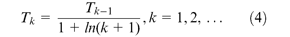
In this article, a new cooling function is developed as equation (4) by redefinition of the logarithmic function. In this function, undesirable increase of the initial temperature at the primary stages of the algorithm is prevented, and a natural logarithm is used to increase the reduction rate. Figure 3 compares the reduction trend of convergence to zero for each function. All initial temperatures are assumed to be 5 °C to be able to compare the reduction trend. It can be observed that the proposed function has a faster reduction rate for temperature. It is important to use the proper function along with other parameters, such as initial temperature and the number of inner loops.

Figure 3.

Comparison of different cooling functions.

$$T_k=\frac{T_{k-1}}{1+\ln (k+1)},k=1,2,\dots$$

(4)

Initial temperature

Initial temperature (T₀) has a high effect on the number of iterations and total optimization time. If the system is cooled down quickly (quenched) or the initial temperature is too low, it does not reach thermal equilibrium and a steady-state, but rather ends up in a polycrystalline or amorphous state having higher energy. Temperature appears in acceptance criterion of the algorithm (Boltzmann distribution function) and the cooling function. It must be large enough to enable the algorithm to move off a local minimum, and small enough not to move off a global minimum. In this article, two important issues have been considered in calculation of the initial temperature. First, the initial temperature is an average value in the range of effective temperatures in the Metropolis acceptance condition, and second, an adaptive method is used for its calculation. In fact, initial temperature shows the highest temperature in the Metropolis algorithm. In order to estimate the initial temperature in this method, the algorithm is allowed to sample 1000 randomly generated values covering the whole search space without considering the failures. Then the initial temperature is obtained by calculating the amplitude of changes for cost functions (CF) or “Energy” for selected samples by equation (5). ⁴³ By this equation, a temperature is selected as the initial temperature with which the number of accepted points to the total points’ ratio (β) is equal to 0.5. It means that 50% of changes are accepted by the Metropolis acceptance condition at this temperature. The designer may restrict or widen this value.

$$T_0=\frac{-(\text{Max}\mathrm{CF}-\text{Min}\mathrm{CF})}{\ln (\beta )}$$

(5)

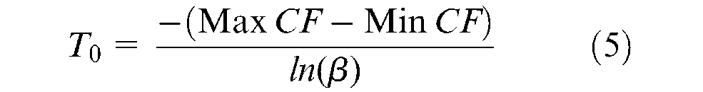
The initial temperature is obtained as 5 °C based on this method.

MCL

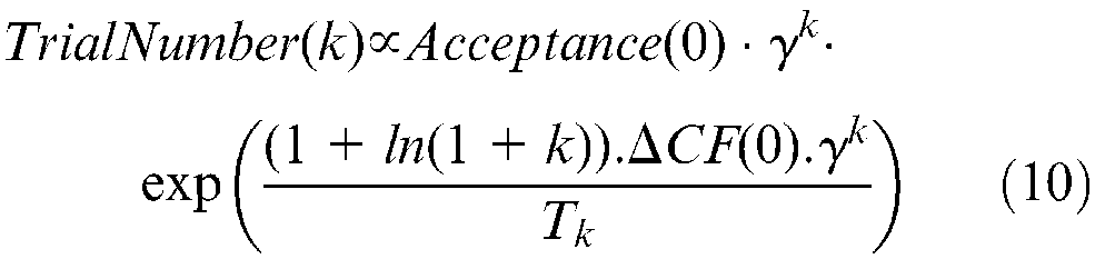
In order to increase the performance of the SA algorithm, there should be a logical balance between speed and accuracy. MCL is the number of iterations in each inner loop that is determined to reach the thermal equilibrium. The simulations (generation, evaluation and acceptation) should be repeated enough times so that the system approaches steady-state at each temperature. MCL might be constant or adaptive. Constant MCL means that there is the same trial number at each temperature, but in fact different iterations are necessary at different temperatures. At high temperatures with higher entropy, there is little chance of finding the appropriate answer. Also, at low temperatures with a low acceptance probability, use of a large number of iterations is not helpful. The middle temperatures range is the most suitable range for performance of the algorithm, so the most trials should be performed at this effective range. In adaptive definition of this parameter, the number of iterations in each inner loop is dependent on other parameters, such as temperature or neighborhood radius. In this article, MCL is defined dependent on the number of acceptances in each loop. The number of acceptances in each Markov chain decreases exponentially proportional to the neighborhood radius. Therefore, considering the Boltzmann distribution function and Metropolis acceptance condition

$$\frac{\mathrm{Acceptan}\mathrm{ce}(k)}{\mathrm{TrialNumber}(k)}\propto \exp \left(\frac{-\Delta \mathrm{CF}(k)}{T_k}\right)$$

(6)

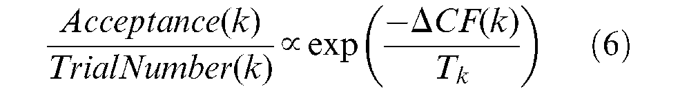
where Acceptance(k) is the required number of acceptances, TrialNumber(k) the necessary iterations to achieve these acceptances, and $\Delta \mathrm{CF}\left(k\right)$ the cost function changes. So

$$\mathrm{TrialNumber}(k)\propto \mathrm{Acceptan}\mathrm{ce}(k)·\exp \left(\frac{\Delta \mathrm{CF}(k)}{T_k}\right)$$

(7)

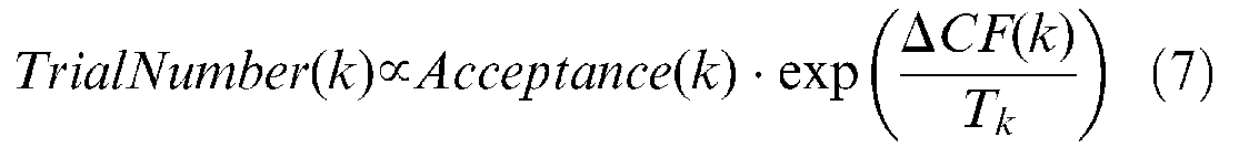
This equation represents the proportion of the number of iterations in the inner loop (MCL) to the needed acceptances, cost function and temperature. In this article, the cost function changes in modeling of the MCL are selected as a descending function with a reduction coefficient close to the unit. So

$$\mathrm{Acceptance}\left(k\right)=\mathrm{Acceptance}\left(0\right).{\gamma }^k$$

(8)

$$\Delta \mathrm{CF}\left(k\right)=\Delta \mathrm{CF}\left(0\right).{\gamma }^k$$

(9)

Considering equation (6)

$$\mathrm{TrialNumber}(k)\propto \mathrm{Acceptan}\mathrm{ce}(0)·{\gamma }^k·\exp \left(\frac{(1+\ln (1+k)).\Delta \mathrm{CF}(0).{\gamma }^k}{T_k}\right)$$

(10)

Combining with equation (5)

$$\mathrm{TrialNumber}(k)\propto \mathrm{Acceptan}\mathrm{ce}(0)·{\gamma }^k·\exp (-\ln (\beta ).(1+\ln (1+k)).{\gamma }^k)$$

(11)

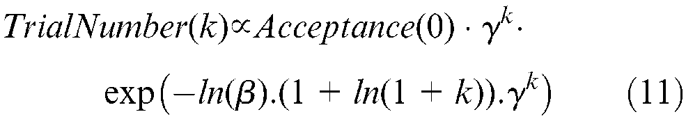
The values of 0.95, 0.5 and 20 are assigned to $\gamma$ , β and Acceptance(0), respectively. The proposed method causes the MCL to adaptively increase at the beginning of the search, and decrease after passing the effective temperature range.

Convergence condition

Definition of the convergence condition is problem dependent. In this article, if the number of outer loops exceeds 25 or $(maxE-minE)<\mathrm{DT}$ the algorithm stops, and the final variables are selected as the optimum values. DT is the desired tolerance, which is selected as 0.0001 here.

Goal function

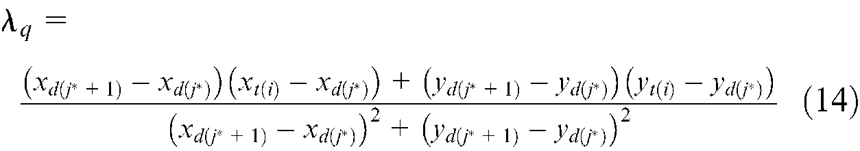
In a WTH process, it is expected to produce non-defective fully formed parts with minimal wall thinning. Therefore, maximum conformation with final geometry after the forming process is assumed to be the goal in this problem. This condition is controlled by checking the distance of each tube node from the die (minimum distance of node from the line) in a FE post-processor. In tube hydroforming, shape nonconformity usually occurs at die corners. The goal function is defined as the total sum of the distances of all upper nodes on tube (the nodes that make contact to the die) from the die. Equation (13) calculates the distance of each upper tube node $p_{t(i)}$ from a line passing through two of its adjacent nodes on the die, $p_{d(j^{*})}$ and $p_{d(j^{*}+1)}$

$$p_{t(i)}=(x_{t\left(i\right)},y_{t\left(i\right)})\text{and}{p}_{d(j^{*})}=(x_{d\left(j^{*}\right)},y_{d\left(j^{*}\right)})$$

(12)

$$d(i,j^{*})=\sqrt{{(x_{t\left(i\right)}-x_{d\left(j^{*}\right)}-{\lambda }_q(x_{d(j^{*}+1)}-x_{d\left(j^{*}\right)}))}^2+{(y_{t\left(i\right)}-y_{d\left(j^{*}\right)}-{\lambda }_q(y_{d(j^{*}+1)}-y_{d\left(j^{*}\right)}))}^2}$$

(13)

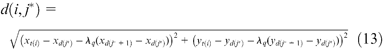
where i is the ith node on tube, j^* is the jth node on the die that has the minimum distance from the ith node on the tube, x and y are coordinates, and t and d are the indices that indicate tube and die, respectively. ${\lambda }_q$ is obtained by

$${\lambda }_q=\frac{(x_{d(j^{*}+1)}-x_{d\left(j^{*}\right)})(x_{t\left(i\right)}-x_{d\left(j^{*}\right)})+(y_{d(j^{*}+1)}-y_{d\left(j^{*}\right)})(y_{t\left(i\right)}-y_{d\left(j^{*}\right)})}{{(x_{d(j^{*}+1)}-x_{d\left(j^{*}\right)})}^2+{(y_{d(j^{*}+1)}-y_{d\left(j^{*}\right)})}^2}$$

(14)

So, the goal function f(p) is defined as equation (15), which has to be minimized

$$f\left(p\right)=\sum _{i=1}^{N}d(i,j^{*})$$

(15)

where N stands for the total number of upper nodes on the tube.

Input variable

The input variable in optimization of WTH is the slope of pressure versus time curve. Total process time (t) is considered as 20 ms in FE simulations. The slope of the loading curve is calculated by

$$s=\frac{\mathrm{Pressure}}{\mathrm{time}}$$

(16)

Accordingly, at each step, by considering a new value for the slope of the pressure diagram, the new energy will be obtained by FE analysis. Finally, the best gradient (with which the minimum goal function is obtained) gives the optimized internal pressure. Pressure is calculated considering an initial value defined by the designer and the neighborhood radius. Neighborhood radius (NR) in the SA algorithm is defined as

$$\mathrm{NR}=0.1\times \frac{\mathrm{UB}-\mathrm{LB}}{2}$$

(17)

where UB and LB are the upper and lower bounds for pressure, respectively. The amount of changes at each step is defined by the neighborhood radius reduction coefficient (NRRC). So the new neighborhood radius at the new temperature is obtained by

$$\mathrm{New}\mathrm{NR}=0.9\times (\mathrm{random}(0,1)-0.5)\times \mathrm{NR}$$

(18)

where random(0,1) is a random real number between 0 and 1.

Fault detection

During the procedure, FE results are checked for the failure criterion. Failure criterion is determined based on the combination of the von-Mises stress and maximum thinning percentage. The process fails if the thinning percentage is more than the maximum allowed thinning (given in Table 1), or the von-Mises stress is higher than the ultimate tensile strength of the material at each temperature. The von-Mises stress and the thinning percentage are calculated and given by a FE post-processor. In case of fault detection, the algorithm generates a new value for the input variable, and the process continues.

The above-mentioned procedure is summarized in Figure 4 showing the optimization package.

Figure 4.

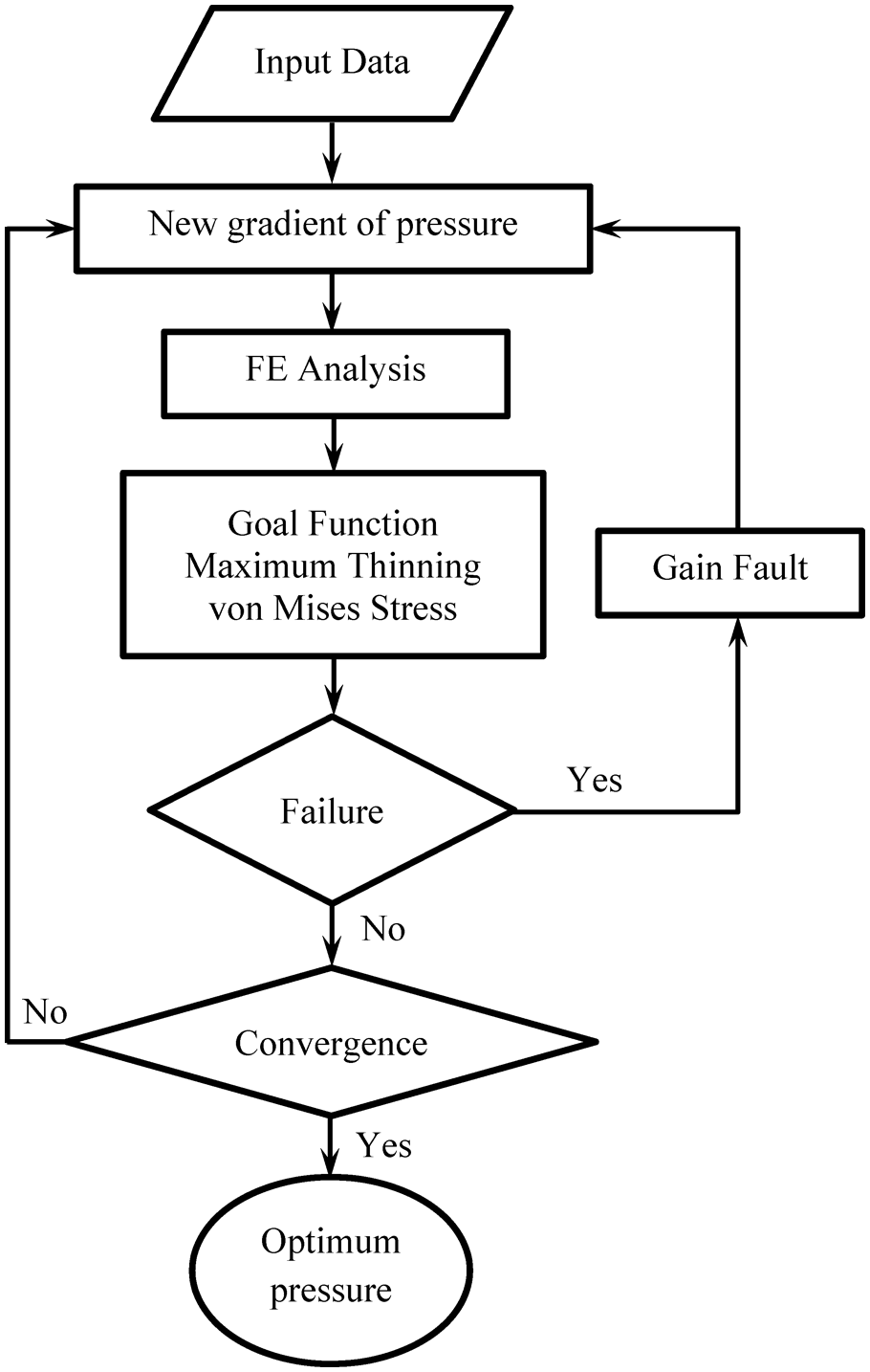
Optimization package flowchart.

Results and discussion

Experiments are performed to validate the numerical results. Experimental set-up is explained in Yi et al. ⁴⁴ A total of 40 different cases, which are summarized in Table 2, were investigated at 300 °C. A 24-mm length tube with an initial diameter of 50.8 mm and final diameter of 66 mm is tried with four different thicknesses (1.5, 3, 5 and 7 mm), and ten different corner radii from r/t = 10 to r/t = 1 are simulated for each thickness. So there are four groups with different thicknesses starting with the highest r/t ratio to the lowest one. Figure 5 summarizes all the results obtained by the optimization process. As predicted by theoretical equations for simple geometries, when the r/t ratio increases, the required internal pressure decreases. On the other hand, in equation (2) – which predicts the maximum needed pressure to form the corner fillets – the effect of the D _i /t ratio is neglected, while equation (1) and the optimized results show that this effect is not negligible. The reduction trend of pressure obtained by theoretical equations and SA is the same, but the optimal values to form the full shape are higher. This shows that theoretical equations are not capable of precise prediction of needed pressure during the forming process. As shown in Figure 5, the correlation coefficient (R²) for each group is very close to 1.00, which reveals the data set is highly precise. Note that the correlation coefficient only confirms the precision, not accuracy. To validate the accuracy of the results, experiments have been performed on Case 21. Case 21 is defined with geometry of D _i /t = 10.16, t = 5, r/t = 10. Figure 6 shows the part produced under optimal conditions. The total process time is 5 s, and the main bulge is formed during the 2nd∼4th seconds, which is called the “forming stage”. The internal pressure amount is constant in this period because when the bulge happens, the volume of product increases and the oil flow is just enough to maintain the pressure. Corner fillets are filled at the “calibration stage”. It is shown that the product is fully formed under the optimized pressure loading path without any processing defects.

Figure 5.

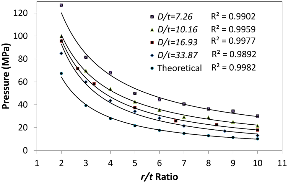
The effect of r/t and D _i /t ratios on internal pressure.

Figure 6.

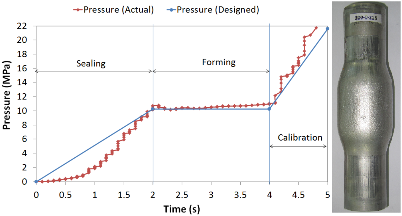
Optimal pressure loading path for Case 21 (D _i /t = 10.16, r/t = 10).

Figure 7 compares the thinning percentage obtained by experiments with a FE. It is observed that FE analysis shows a higher amount of thinning than the actual experiments. As explained before, this difference is because of the complicated nature of forming at elevated temperatures, mainly owing to the differences in strain rate, friction conditions and temperature gradient during the process.

Figure 7.

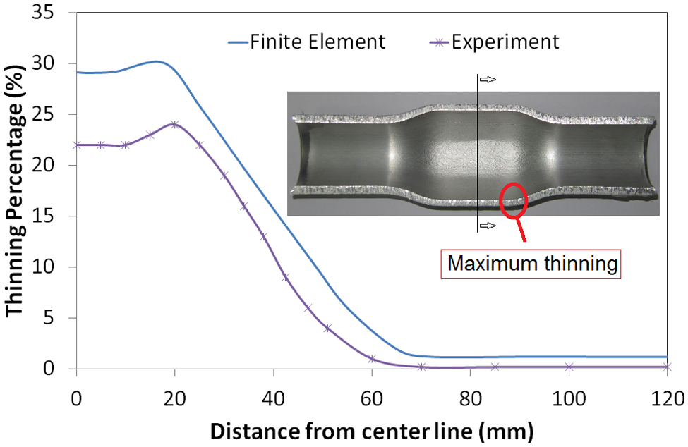
Comparison of the thinning in experiments and simulations.

The iteration versus goal function diagram gives an estimation of how well the initial variables and search space are determined. In this article, knowing the fact that the reduction of the r/t ratio increases the required internal pressure, the optimum pressure in each case is used as the lower bound for the next case in each group with the same D _i /t ratio. For the first case of each group, which has the highest r/t ratio (r/t = 10), and hence the lowest needed pressure, the lower bound is defined according to equation (1). It means that the search space in the first case is larger than other cases. So the algorithm converges to the optimal response faster in cases other than the first one since the search space is smaller, and the initial guess is more precise. This fact is shown in Figures 8 and 9 as an example. Figure 8 represents this diagram for the first case of the second group, Case 21 (D _i /t = 10.16, r/t = 10), in which there is a large difference between the primary value and optimal one; while, Figure 9 shows the curve for another sample, Case 15 (with geometry of D _i /t = 16.93, r/t =7), in which the initial variable is well defined, and it converges to the optimal response much faster. Hence, the number of iterations for the Case 15 is 155, while for the Case 21 is 199. Note that the scale of vertical axis in Figure 8 is “mm” while in Figure 9 it is “×10⁻⁴mm”. From an engineering point of view, the designer may decide to stop the algorithm when it gets close to 0, e.g. in Figure 8, after about 55 iterations, the goal function converges to near zero. This will help the engineers the save more time and cost.

Figure 8.

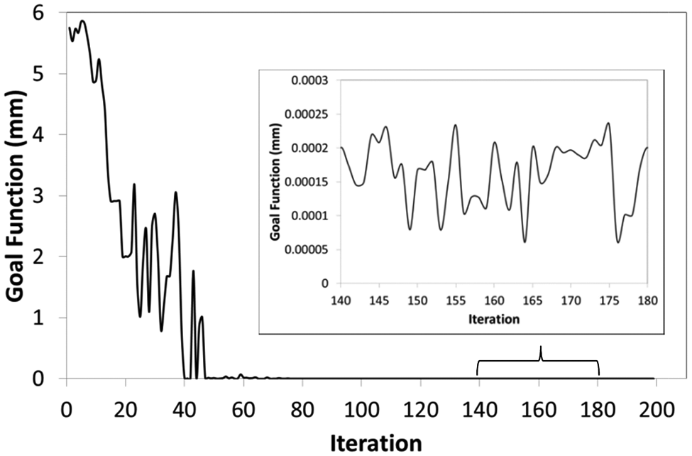
Iteration versus goal function for Case 21 (D _i /t = 10.16, r/t = 10).

Figure 9.

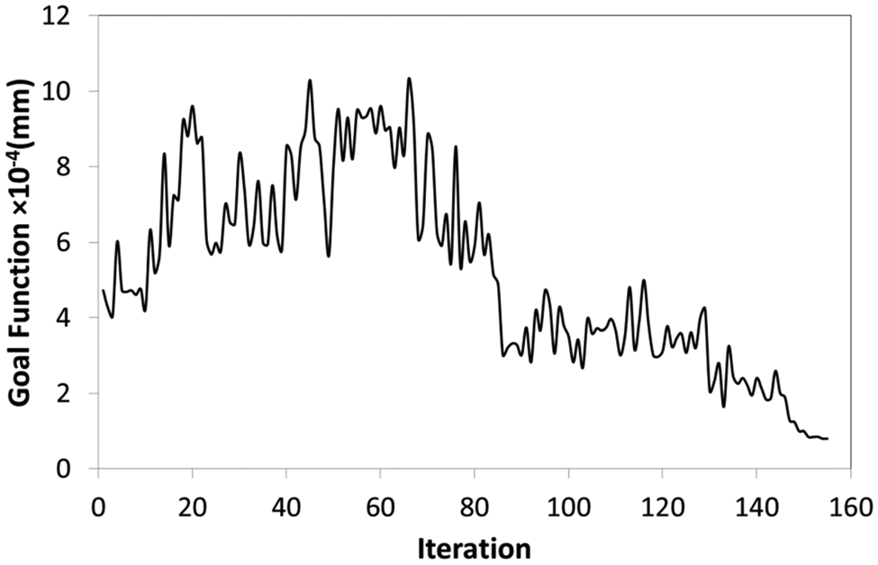
Iteration versus goal function for Case 15 (D _i /t = 16.93, r/t =7).

As an advantage for this technique, the simultaneous interaction of the FE code (ANSYS/Ls-Dyna) and SA code enables this method to verify the results numerically through the fault detection stage. So there is no possibility for any error in solving this problem. As shown in Figures 8 and 9, the only disadvantage for this method is its high dependency on initial process definitions, such as the annealing schedule and initial variables’ values.

Conclusion

A SA algorithm is used as a new technique in optimizing the pressure loading path in the WTH process. Optimized results are numerically and experimentally verified. The SA method is a problem-dependent technique in which all critical definitions, such as cooling schedule, initial temperature, initial variables, and upper and lower bounds, have to be determined for each specific problem. A new adaptive cooling schedule is proposed to increase the rate of convergence to the global minima. Furthermore, an adaptive method is used for determination of the initial temperature. Using the results of each simulation as the initial variables for the next case, the number of iterations and total solution time is significantly reduced.