Sage Journals: Discover world-class research

Abstract

Recent development of electrically assisted manufacturing processes proved the advantages of using the electric current, mainly related with the decrease in the mechanical forming load, and improvement in the formability when electrically assisted forming of metals. The reduction of forming load was formulated previously assuming that a part of the electrical energy input is dissipated into heat, thus producing thermal softening of the material, while the remaining component directly aids the plastic deformation. The fraction of electrical energy applied, which assists the deformation process compared to the total amount of electrical energy, is given by the electroplastic effect coefficient.

The objective of the current research is to investigate the complex effect of the electricity applied during deformation, and to establish a methodology for quantifying the electroplastic effect coefficient. Temperature behavior is observed for varying levels of deformation and previous cold work. Results are used to refine the understanding of the electroplastic effect coefficient, and a new relationship, in the form of a power law, is derived. This model is validated under independent experiments in Grade 2 (commercially pure) and Grade 5 (Ti–6Al–4V) titanium.

Keywords

Electrically assisted forming electroplastic effect resistive heating titanium

Introduction

Lightweight manufacturing in automobiles

Since it is expensive and processing-intensive, titanium is usually reserved for use in either aircraft or motorsport applications that demand high performance. Titanium is currently not desired as a “mass production” material because of high cost and limited formability.

Lower-cost titanium alloys for use in the automotive industry are being developed to give feasible raw material options to more cost-sensitive industries. Other lightweight metals, such as magnesium and aluminum, are already in more widespread use in the automotive industry, as requirements for higher fuel efficiency drive lower-mass designs. However, the use of these materials is coupled with the need for cost-efficient manufacturing processes. Presently, titanium and its alloys are limited in forming by energy-intensive and expensive processing, or limited formability when deformed. A new class of electromechanical processing, known as electrically assisted manufacturing (EAM), has shown the potential for higher achievable deformation with a lower energy requirement than that of competing processes. However, a better understanding of the effect of electrically assisted forming (EAF) (a specific type of EAM) is warranted, particularly the partitioning of thermal softening and direct electrical flow stress reduction.

EAM

EAM is a recently introduced metal forming technique capable of enhancing a metal’s formability during deformation.¹ In this technique, electricity is applied to the metal blank or billet while it is deformed, without stopping deformation. EAF is a specific type of EAM. A schematic of an EAF test set-up can be seen in Figure 1.²

The multiple benefits generated from the applied electricity are collectively known as the electroplastic effect. The three main benefits of the electroplastic effect are as follows.

Reduction in the flow stress required to continue plastic deformation.

Increased achievable part deformation prior to failure.

Reduction/elimination of springback effects in formed parts.

Figure 1.

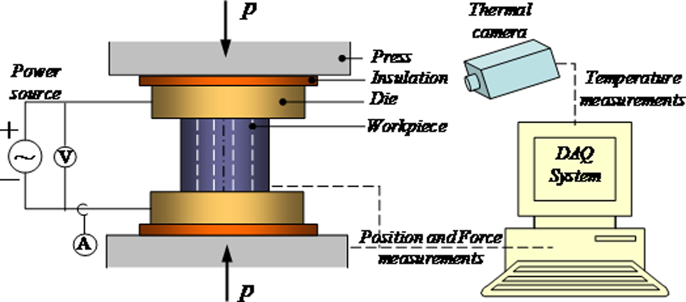
Schematic of an EAF test set-up.

Figure 2 displays EAF’s ability to transform strong and fairly brittle Ti–6Al–4V into a highly formable material. The specimens in the figure are some of the Ti–G5 specimens used in this work. In Figure 2(a), a specimen compressed under conventional conditions, with no applied electricity, is shown. After a minimal amount of deformation, the material failed due to shear fracture. Figure 2(b) shows a specimen compressed under EAF conditions, where the electricity was applied for the duration of the test. Owing to the electricity, the part was able to be formed to its desired height without failure. Details on the process conditions are given farther in the experimental section.

Figure 2.

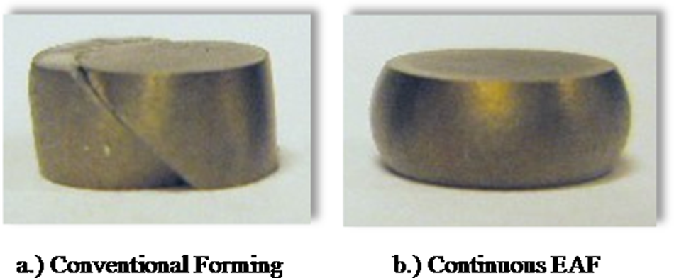
EAF formability improvement (TI–G5).

Development of EAM

In 1959, Machlin examined electricity’s effect on group 1A salts (NaCl), concluding that the electrical current notably affected the ductility, flow stress, and yield strength of the material.³ Later, in 1967, Nabarro devoted a chapter of his book towards electricity’s effect on metals, discussing charged dislocations, electrostatic fields, and presenting a materials-based equation for electrical resistivity.⁴ Troitskii et al., in 1969, researched the influence of electrons on dislocation creation and movement in different alloys of zinc, tin, lead, and indium, determining that flow stress could be reduced using high-current pulsed electricity.⁵ Okazaki et al., in 1978, studied the effect that pulsed electricity had on materials of different crystalline structures in uniaxial tension and found that the order of responsiveness to the electroplastic effect of the materials is similar to the order for a normal-to-superconducting transition.⁶ This supports the claim that both effects may reflect comparable types of electron-dislocation interaction. Afterwards in 1982, Klimov and Novikov proposed that an electric current may have a specific effect on a metal’s structure that is not the result of Joule heating.⁷ Work by Xu et al. in 1988 examined the recrystallization and grain growth behavior of pre-worked Ti plate when exposed to long durations of low current electricity.⁸ In 1998, Chen et al. developed a relationship between electric flow and the formation of intermetallic compounds (Sn/Cu and Sn/Ni systems).⁹ Then, Conrad (2002) determined that the plasticity and phase transformations of metals and ceramics are affected by very high-current density, short-duration electrical pulses.¹⁰

In 2007, Andrawes et al. was able to conclude that an electrical current can significantly reduce the required deformation energies without excessively heating the workpiece when in uniaxial tension.¹¹ Additionally in 2007, Perkins et al. produced an experimental EAM compression work, which presented results from formability-enhancing EAM compression tests on many types of popular engineering metals.¹² Ross et al. (2007) performed the same type of study in tension.¹³ From this, it was concluded that continuously applied electricity reduced the flow stress, but consequently also reduced achievable tensile elongation. This work proved that different electrical application methods were optimum for specific types of deformation. Further descriptions of these and other works on EAM can be found in Salandro and Roth.¹

More recently, work has been done to not only experimentally prove EAM’s effects, but also begin to understand and model various aspects of EAM and its level of effectiveness. Siopis et al.^14,15 examined how different microstructure properties affect the effectiveness of EAM in micro-extrusion experiments. Specifically, it was concluded that a finer-grained material, with more grain boundary area, enhanced the electroplastic effect, whereas a larger-grained material, with less grain boundary area, lessened the effect.¹⁴ Another work by Siopis et al. (2009) determined that the effectiveness of EAF increased as the dislocation density within the metal also increased, as a result of cold-working prior to EAF experiments.¹⁵ Further, research by Dzialo et al. (2010) showed that, above the critical threshold current density, the efficiency of the applied electricity increased with the percentage of alloyed Zn in copper specimens during microforming.¹⁶

There have been several previous works which strived to model an EAM process. Specifically, research by Kronenberger et al. (2009) showed that an FEA model, accounting strictly for resistive heating effects, proved unsuccessful in modeling an EAM process.¹⁷ Additionally, Ross et al. (2009) proved that the forming flow stress profiles for an EAM compression test and an isothermal compression test (at the maximum temperature reached during the EAM test) were considerably different.¹⁸ Both of these works support the theory that the applied electricity during an EAM process has direct dislocation effects aside from just resistively heating the workpiece. To this end, work by the authors has been done on modeling various EAF processes and their attributes. In Bunget et al.,² an approach for modeling the flow stress of an electrically assisted forging process was presented, where the electrical power was separated into heating and deformation effects using a newly adopted electroplastic effect coefficient (EEC). This coefficient designates the specific efficiency of the electricity used to enhance deformation. In Salandro et al.,¹⁹ a similar modeling approach was used to model an electrically assisted air bending process. Since pulsing the electricity is most effective in tension-based processes, a piece-wise model was used to simulate pulsing the current. In these two previous works, a complete thermal energy balance was also included in the models, which accounted for conduction, convection, and radiation heat transfer. This balance is the basis for the thermal model presented in this research.

Objective and approach

The objective of the current research is to investigate the complex effect of the electric current applied during deformation, and to establish a methodology for quantifying the electroplastic effect coefficient. This coefficient is defined as the fraction of electrical energy applied that assists the deformation process compared to the total amount of electrical energy. From the conservation of energy and empirical observations, an analytical model able to predict the temperature rise in the specimen owing to the electricity that was applied while subjected to deformation, is proposed. The formulation of the EEC is projected to be a function of material and electric field parameters, as well as prior cold work.

The authors previously formulated a simplified thermo-mechanical model for predicting the stress–strain variation for an electrically assisted compression test.² That model assumed the EEC to be constant during the duration of the forming test. In this present work, further refinement is proposed for the electroplastic effect coefficient. Let it be known that the EEC is dependent on the magnitude of current applied to the workpiece. Since the purpose of this work was to develop a preliminary model and propose a procedure for determining the electroplastic effect coefficient, only one current magnitude was used.

Methodology

Aspects of the electroplastic effect

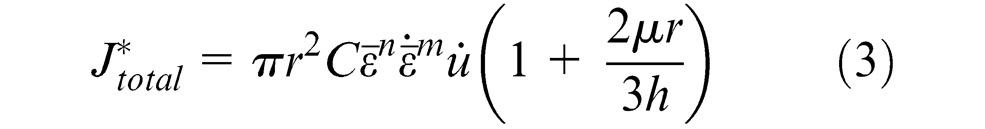
The application of electricity to a metallic part during plastic deformation is a complex phenomenon. The electric energy consumed results in an increase in the specimen’s temperature and in the dies near the vicinity of the part. The resistive heating of the specimen results in thermal softening of the material, thus the flow stress decreases. Previous thermal measurements have proven that the temperature rise is lower than expected from the balance of energies. Furthermore, Ross et al.¹⁸ investigated the reduction in the forming load in an electrically assisted test and compared it to deformation experiments where the workpiece was at similarly high temperatures. Their observations led to the conclusion that the decrease in the forming load in the electrically assisted test is higher than what can be attributed solely to the thermal softening effect. This difference is attributed to the electroplastic effect, which is the fraction of the electric energy imparted into the mechanical deformation process, as follows

P_{e} = P_{heat} + P_{def} = η (1 - ξ) VI + η ξ VI

(1)

where P_e is the electric power (I.V), η is the efficiency, and ξ is the EEC.^2,19P_hea_t represents the amount of electric power that will dissipate into heat through resistive heating of the workpiece. P_def is the electrical power component that will aid the plastic deformation. As a result, the decrease in the force needed for the same deformation as in a conventional test (at room temperature), is controlled by two mechanisms: (a) thermal softening, thus lower flow stress, and (b) facilitating deformation owing to the energy provided by the electrons to the dislocations, as well as indirect effect of the resistive heating.

Using the thermo-mechanical model previously developed by the authors for electrically assisted compression, the stress–strain distribution can be determined.² In the development of the model, the component of the electrical energy that goes into aiding deformation, as defined in equation (1) is integrated into the governing equation, as follows

J_{total}^{*} = J_{m}^{*} + J_{e}^{*}

(2)

where $J_{m}^{*}$ is the mechanical component, and $J_{e}^{*}$ is the electrical component, which is equivalent to P_def in equation (1). The total power consumed by the process and the individual components are given by

J_{total}^{*} = π r^{2} C {\bar{ε}}^{n} {\overset{\cdot}{\bar{ε}}}^{m} \overset{\cdot}{u} (1 + \frac{2 μ r}{3 h})

(3)

J_{m}^{*} = π r^{2} p \overset{\cdot}{u}

(4)

J_{e}^{*} = η ξ VI

(5)

where C is the strength coefficient of the material, $\bar{ε}$ and $\overset{\cdot}{\bar{ε}}$ are the effective strain and strain rate, n is strain hardening exponent, m is the strain rate sensitivity, p is the pressure exerted by the die, $\overset{\cdot}{u}$ is the die speed, r and h are the instantaneous part dimensions, and µ is the friction coefficient. The overall model is written as

π r^{2} C {\bar{ε}}^{n} {\overset{\cdot}{\bar{ε}}}^{m} \overset{\cdot}{u} (1 + \frac{2 μ r}{3 h}) = π r^{2} p \overset{\cdot}{u} + η ξ VI

(6)

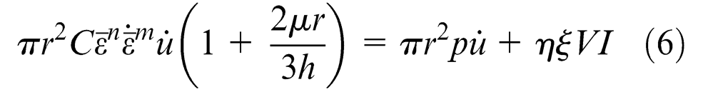
with ξ formulated from the thermal model. The model can be solved to determine the pressure, p, needed for deformation, which can be further used to calculate the stresses. Note that this forming pressure is reduced when electricity is used, as compared to the conventional test. This reduction is comprised by the electroplastic effect coefficient, which needs to be accurately predicted, as well as the temperature variation in EAF, since C,n, and m are material parameters dependent on the temperature.

The EEC depends on specific material properties, such as heat capacity, electric resistivity, electric field characteristics, contact pressure at the die/workpiece interfaces, and the prior cold work of the initial specimen. The next sections will investigate all these aspects. But first, the development of an analytical model for predicting the temperature rise in the specimen owing to the applied electricity presented.

Assumptions of the thermal model

Simplifying assumptions were used to facilitate the derivation of the model, as follows.

The material is homogeneous and isotropic.

The increase in temperature owing to friction at the workpiece/die interface is negligible. This assumption is valid for the small dimensions and low relative speeds in the compression tests.

The barreling effect owing to friction is neglected when the model is solved.

In the initial calculations, the material properties that are assumed constant with temperature are C_p and ρ. The influence of material property changes will be discussed.

The temperature distribution in the part is considered uniform. In reality, contact resistance under low loading causes an increase in the temperature at the ends of the specimen at the beginning of application, followed rapidly by homogeneous heating as the load increases and contact resistance effect becomes negligible. The outside boundaries will also have a different temperature distribution, and these boundary conditions will be taken into consideration when the solution for the model is calculated.

The voltage in the specimen is assumed constant and it is determined for the initial dimensions of the specimen at room temperature. However, the voltage will vary during the test. On one hand the decrease of the ratio of height over cross-sectional area results in lower resistance, thus lower voltage, while the increase in temperature will increase the resistivity, thus resistance and voltage increase. Overall, the present work assumes that these effects cancel each other.

The temperature rise and its distribution during an electrical test are illustrated in Figure 3 during a stationary test, where electricity is applied without plastic deformation. It can be seen that the specimen heats up rapidly for about the first 12 s, until the electricity is shut off. Then, the heat from the specimen conducts into the compression dies.

Figure 3.

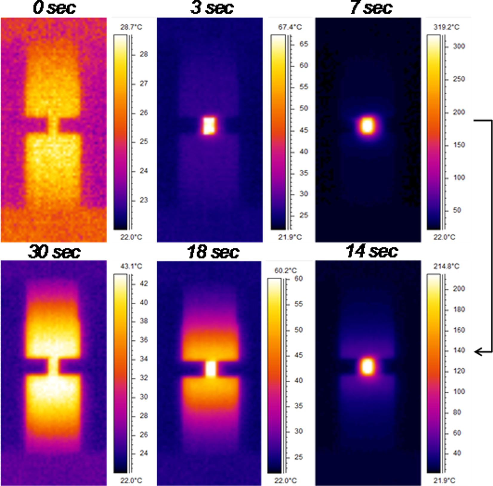
Heating and cooling sequence during a stationary electrical test.

When examining only the specimen, the specific temperature profile will also change throughout the test. More specifically, the temperature of the die/workpiece contact points at the beginning of the test will be much hotter than the rest of the specimen (because the actual contact area will be less, leading to a higher overall electrical power at these points). However, as the part is compressed and the asperities are crushed, the temperature profile inverts and the middle of the specimen is the hottest (since the asperities crush and the contact area increases, leading to a decrease in the electrical power at these points). The estimated thermal profiles are illustrated in Figure 4.

Figure 4.

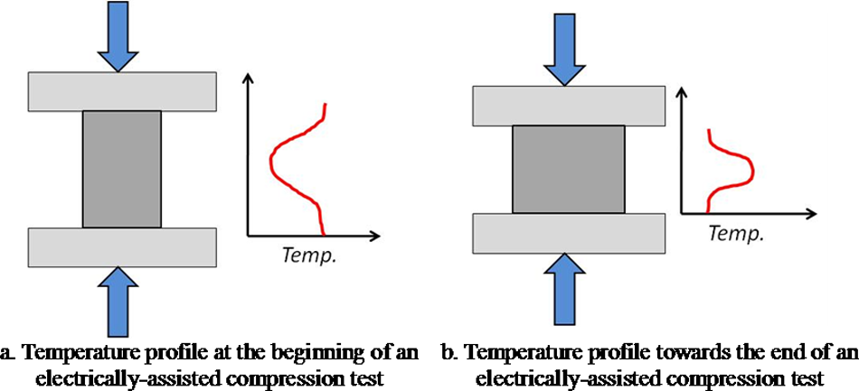
Specimen thermal profiles at the beginning and end of an electrically assisted compression test. (a) Temperature profile at the beginning of an electrically assisted compression test. (b) Temperature profile towards the end of an electrically assisted compression test.

Development of the thermal analytical model

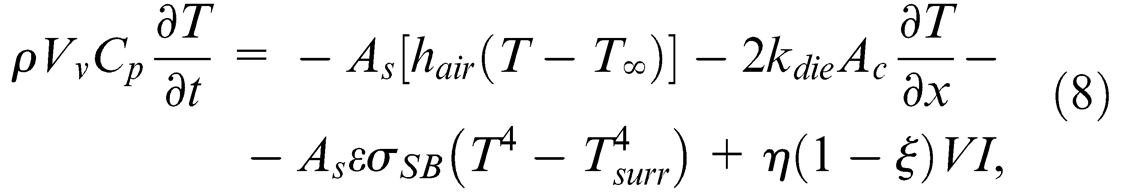
For a better understanding of the electroplastic effect, the thermal aspects have to be isolated. When the electric current passes through the metallic workpiece, heat is generated and the temperature of the part rises. The temperature increase is determined from the energy balance, shown in Figure 5.

The general form of the energy conservation is expressed on a rate basis as

\begin{matrix} {\overset{\cdot}{E}}_{part} = {\overset{\cdot}{E}}_{g} - {\overset{\cdot}{E}}_{out}, \\ \overset{\cdot}{Q} = {\overset{\cdot}{Q}}_{e} - {\overset{\cdot}{Q}}_{cond} - {\overset{\cdot}{Q}}_{conv} - {\overset{\cdot}{Q}}_{rad}, \end{matrix}

(7)

Figure 5.

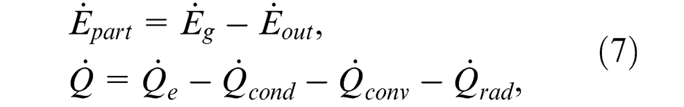
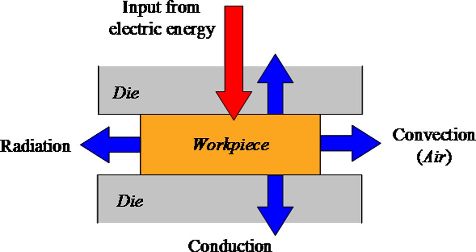
Heat flux energy balance.

where ${\overset{\cdot}{E}}_{part}$ is the rate of change of the energy content in the part analyzed ( $\overset{\cdot}{Q}$ ), ${\overset{\cdot}{E}}_{g}$ is the rate of heat generation owing to the electric resistive heating ( ${\overset{\cdot}{Q}}_{e}$ ), and ${\overset{\cdot}{E}}_{out}$ is the rate of energy leaving the part owing to conduction into the dies in the contact zone ( ${\overset{\cdot}{Q}}_{cond}$ ), convection ( ${\overset{\cdot}{Q}}_{conv}$ ), and radiation from the surface ( ${\overset{\cdot}{Q}}_{rad}$ ). After developing each component, the heat equation can be written in one dimension as

\begin{matrix} ρ V_{v} C_{p} \frac{\partial T}{\partial t} = - A_{s} [h_{air} (T - T_{\infty})] - 2 k_{die} A_{c} \frac{\partial T}{\partial x} - \\ - A_{s} ε σ_{SB} (T^{4} - T_{surr}^{4}) + η (1 - ξ) VI, \end{matrix}

(8)

where $ρ$ is the density of the material, $V_{v}$ is the volume of the part, C_p is the specific heat of the material, T is the temperature, t is time, A_s is the lateral surface area of the part, h_air is the convection heat transfer coefficient, $T_{\infty}$ = T_surr is the surrounding temperature, k_die is thermal conductivity for the die material, A_c is the cross-sectional area, x is coordinate, $ε$ is radiative emissivity for the part, and $σ_{SB}$ is the Stefan–Boltzmann constant. The input from electricity was taken from equation (1). The changes in geometry are calculated assuming compression at constant speed, as well as volume constancy, as given by the following equations

\frac{\partial h}{\partial t} = - \overset{\cdot}{u}; \frac{\partial D}{\partial t} = \sqrt{\frac{V_{v}}{π}} \frac{\overset{\cdot}{u}}{h \sqrt{h}}

(9)

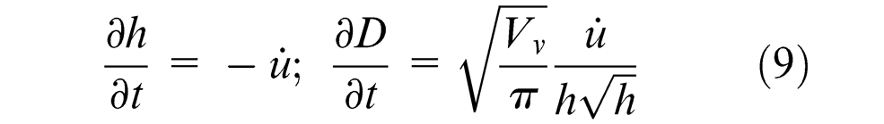
where D and h are instantaneous dimensions of the workpiece, and $\overset{\cdot}{u}$ is the compression speed. The second equation was determined from the volume constancy condition ( $V_{v} = π D^{2} h / π D^{2} h 4 4$ ).

The variation of the temperature of the specimen in time is solved from equations (8) and (9), and combined with experimental thermal measurements and with geometrical changes occurring during the deformation process, the EEC is determined. The procedure is described below.

Solve the model for a stationary test. This is a test when the part is clamped between the dies and pre-loaded, and electricity is applied. The dies are stationary, thus no plastic deformation occurs and the dimensions of the part are not changed.

Validate the model by comparing with thermal measurements from experiments (i.e. strictly resistive heating).

Solve equations (8) and (9) for an electrically assisted deformation test. Note that just the temperature rise component is considered owing to the application of electricity. Initially assume the EEC to be ξ = 0.

Compare the solution from the previous step with the thermal measurements. At this step, the increase in temperature owing to electricity is separated from the increase owing to plastic deformation by subtracting the temperature increase recorded during conventional compression experiments. As will be shown in the results section, there will be a significant thermal profile difference between the experiment and the model. This difference proves the concept of the electroplastic effect coefficient.

Determine the electroplastic effect coefficient, ξ, in order to match the model with the experimental thermal profile, and propose a formulation for this coefficient for the different materials studied.

Further refine the EEC and the model to account for prior cold work.

The analytical model is solved and validated in the next sections, followed by investigations of influencing parameters initially assumed constant, such as material properties as a function of temperature, and contact pressure. Additionally, the effect of prior cold work, which has significant thermo-mechanical effects, will be explored.

Experimental set-up and procedure

The experimental objectives of this work are to:

determine the flow stress reductions due to EAF;

measure the thermal profile during the EAF test;

establish the effect that prior cold work has on the force and temperature profiles for different levels of deformation;

analyze the heating effects in relation to the die contact pressure.

Figure 6 displays the experimental set-up. An Instron Model 1332 hydraulic testing machine was used to compress the specimens. Machined, hardened, and insulated dies, made from A2 tool steel, were installed in the Instron machine (note that insulation was used such to isolate the electricity from the test machine). For thermal measurements, a Flir A40M thermal camera, with a temperature capacity of 550 °C, resolution of 0.1 °C, and a sample frequency of 50 Hz was utilized. All force and position data were gathered using an on-board data acquisition system at 1500 Hz sampling frequency.

Figure 6.

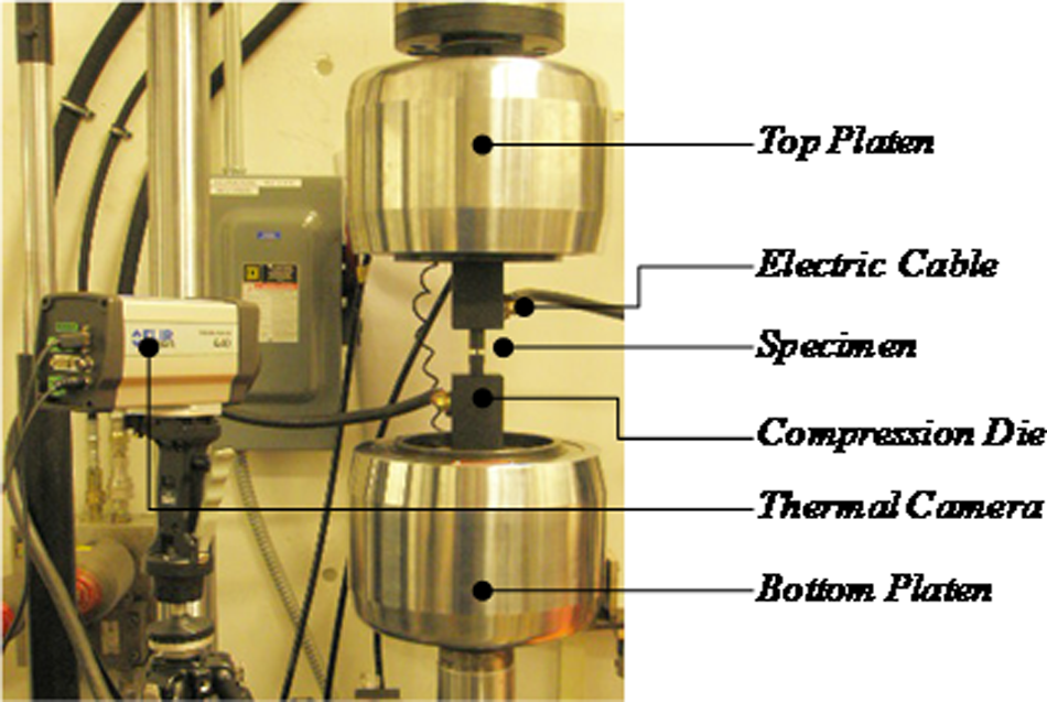
Experimental test set-up.

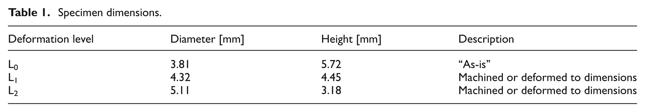
The materials tested are two grades of titanium: Grade 2, which is a single-phase polycrystalline material, and Grade 5 (Ti–6Al–4V), a dual-phase alpha–beta alloy. The initial dimensions of the specimens are summarized in Table 1. A displacement speed of 12.7 mm/min was used for all tests and a constant DC current of 300 A was utilized for all the EAF tests. Please note that, since the cross-sectional areas between the specimens of the three levels of deformation will be different, the resulting current densities will also be different. Considering the size of the “as-is” specimens, the current density supplied to the workpieces is about 26 A/mm², which is above the threshold current density of about 20 A/mm² determined by Perkins et al.¹²

Table 1.

Specimen dimensions.

Deformation level	Diameter [mm]	Height [mm]	Description
L₀	3.81	5.72	“As-is”
L₁	4.32	4.45	Machined or deformed to dimensions
L₂	5.11	3.18	Machined or deformed to dimensions

All specimens used in this work were machined from the same 6.35 mm-diameter rod of each respective material. To account for the “cold working” effect while also keeping the base material consistent, this rod was cut and centerless ground to the specified part diameters. Then, using electrodischarge machining (EDM) processing, the different diameter rods were parted into compression slugs representing L₀, L₁, and L₂ dimensions. This enables a slug machined to L₁ or L₂ (with no prior cold work) to be compared to a L₀ slug that was deformed to L₁ or L₂ (with certain level of cold work). A schematic of this procedure can be seen in Figure 7.

Figure 7.

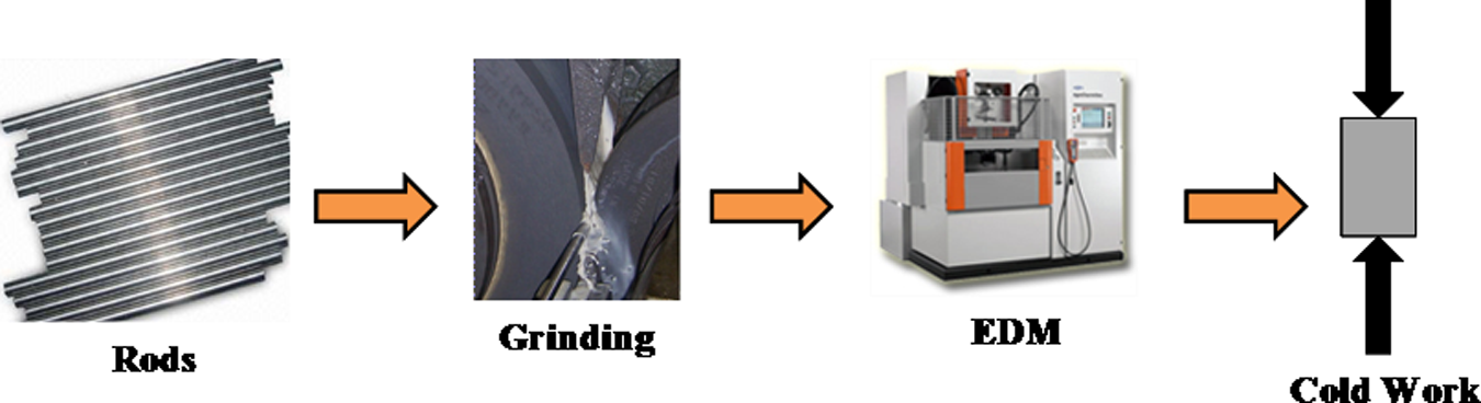
Specimen preparation procedure.

Two types of tests were performed in this work. First, deformation tests were run, where the specimens were deformed at a constant die speed to deformation levels L₁ or L₂, with and without electricity applied. Stress–strain and thermal profiles were created from these tests. Second, stationary tests were performed, where electricity was applied to a specimen without plastic deformation. Specifically, the dies were in contact with the specimen so as to allow electricity to flow, but without causing plastic deformation in the sample. Thermal profiles were gathered from these tests and were used in comparison with each other and with the thermal profiles from the deformation tests, as will be shown in the Results and discussion section. The different test combinations and corresponding specifications can be seen in Table 2.

Table 2.

Test combinations and specifications.

Grade	Deformed/stationary	EAF/conventional	Displacement	Previous structure	% CW
2	Deformed	EAF	L₀-L₂	As-is	–
2	Deformed	Conventional	L₀-L₂	As-is	–
5	Deformed	EAF	L₀-L₂	As-is	–
5	Deformed	Conventional	L₀-L₂	As-is	–
2	Deformed	EAF	L₁-L₂	Initially deformed to L₁	22
2	Deformed	Conventional	L₁-L₂	Initially deformed to L₁	22
2	Deformed	EAF	L₁-L₂	Initially machined to L₁	–
2	Deformed	Conventional	L₁-L₂	Initially machined to L₁	–
2	Stationary	EAF	L₁	Initially deformed to L₁	22
2	Stationary	EAF	L₁	Initially machined to L₁	–
2	Stationary	EAF	L₂	Initially deformed to L₂	44
2	Stationary	EAF	L₂	Initially machined to L₂	–
5	Stationary	EAF	L₁	Initially deformed to L₁	22
5	Stationary	EAF	L₁	Initially machined to L₁	–
5	Stationary	EAF	L₂	Initially deformed to L₂	44
5	Stationary	EAF	L₂	Initially machined to L₂	–

Results and discussion

Within this section, true stress–strain plots and temperature plots will be used to emphasize several EAF relations and effects. First, the reductions in flow stress owing to EAF will be shown. Of note is that, since this work focused on modeling EAF, only one current was used, so the reductions in flow stress from EAF could be much greater if larger currents were utilized. Second, the model prediction process and accompanying experimental results are discussed. The steps required for model prediction are outlined in the Methodology section. Third, an experimental study on the effect of the cold working on EAF performance will be conducted. Fourth, the effect that the contact force, between the dies and specimen, has on the thermal effect of EAF is illustrated. Fifth, changes in material properties owing to elevated temperatures are discussed and shown. From the creation of the model and analysis of several of the main input variables, EAF can be better understood and more accurately predicted through this variety of influencing factors.

Force reduction owing to EAF

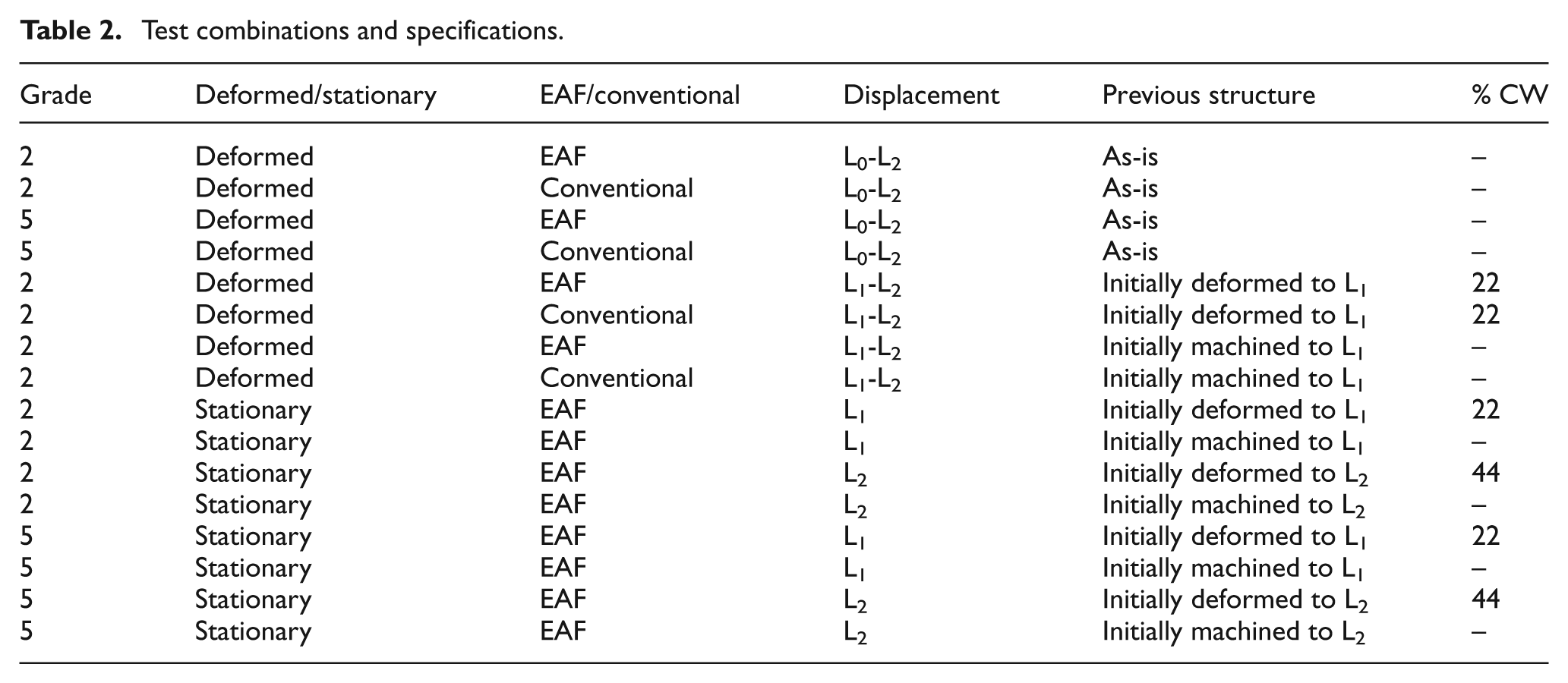
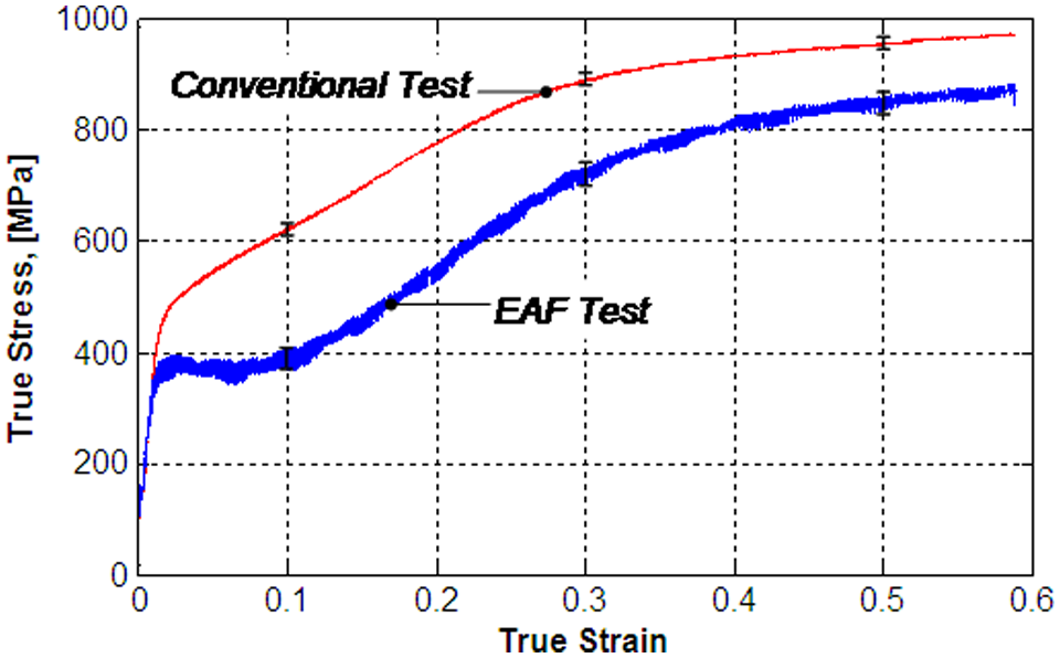
From many experimental works over the last several years, it has been proven that EAF can reduce a metal’s flow stress compared to conventional forming.¹²Figures 8 and 9 show the true stress–strain profiles of a conventional compression test (at room temperature) and an EAF test for Ti–G2 and Ti–G5, respectively. A die speed of 12.7 mm/min was used and a constant current of 300 A was applied during the EAF test. Both figures show that the flow stress was reduced significantly owing to EAF. In Figure 8, one can see that the difference in the flow stress is fairly consistent throughout the test. Conversely, in Figure 9, the difference in flow stress increased slightly as the test progressed. Additionally, the Ti–G5 in the conventional compression test failed before the end of the test. However, in the electrically assisted compression test, the material was able to be completely formed without failure (specimens in Figure 2). The results in Figure 9 are comparable to EAF compression test results of the same alloy run by Perkins et al.¹² Specifically, a small amount of strain weakening is apparent at the beginning of the test, and in both works, the elongation of Ti–G5 is increased using EAF.

Figure 8.

Flow stress reduction owing to EAF (G2).

Figure 9.

Flow stress reduction owing to EAF (G5).

Another observation is that, although the displacement varies linearly in time owing to a constant die speed, the force for the EAF test showed some variation (“noise”). The frequency analysis of the data indicated a frequency response at ∼22.29 Hz and its multiples for G2, and 1.02 Hz and its multiples for G5, which are not found in the conventional tests. The behavior observed may be due to a cyclic softening/hardening phenomenon present during EAF. The input of electric energy results in an alternating of electroplastic softening of the material (thus reduction in the forming load), and hardening of the material owing to deformation (thus increase in load).

Model prediction and experiments

When the electric current passes through a metallic workpiece, heat is generated and the temperature of the part rises. For a better understanding of the electroplastic effect, the thermal aspect needs to be isolated. Two types of EAF tests were performed: (a) deformation test, and (b) stationary test, where the specimen is placed between the dies, while no plastic deformation takes place.

The first step in the model prediction process is to compare the model to a simple stationary test, to isolate the resistive heating effects and validate that the heat transfer relationships within the model are correct. Figure 10 displays both an experimental test and the model output for a stationary test on Ti–G2. The model tends to slightly underestimate the temperatures in the middle of the test, but is extremely accurate at the beginning and end of the test. Additionally, the heating profile of the model is slower than that of the experiments.

Figure 10.

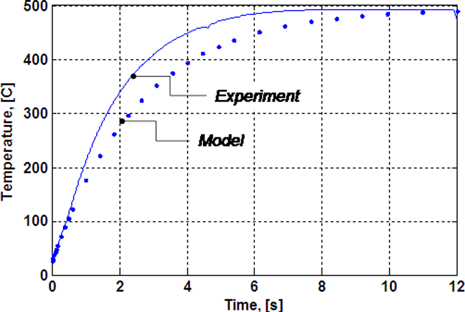
Stationary test at L₀ (G2).

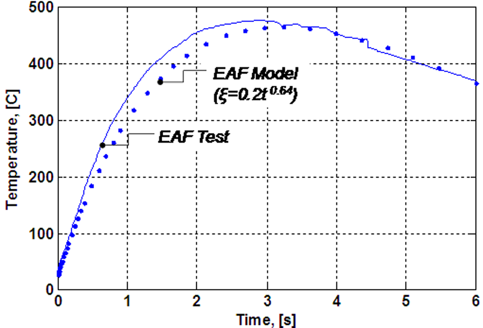
Now that the model can effectively predict resistive heating effects, the effect of plastic deformation must now be included to represent an actual EAF test. The temperatures recorded are presented in Figure 11 for Ti–G2. The EAF deformation test is compared with the stationary tests for intermediate stages of deformation, (i.e. 6 s for L₁ and 12 s for L₂). The temperatures generated during stationary tests owing to resistive heating are extremely greater than the EAF deformation tests. The difference cannot be explained simply by the very small difference in the cross-sectional area (the machined specimens do not have barreling), but by the difference in the dislocation density. Moreover, during the EAF deformation test, a significant portion of the electric energy goes toward assisting plastic deformation, rather than direct resistive heating. Knowing this, the EEC can be determined from the difference in thermal profiles of the model and experimental EAF tests, after deducting the temperature profile for the conventional forming test.

Figure 11.

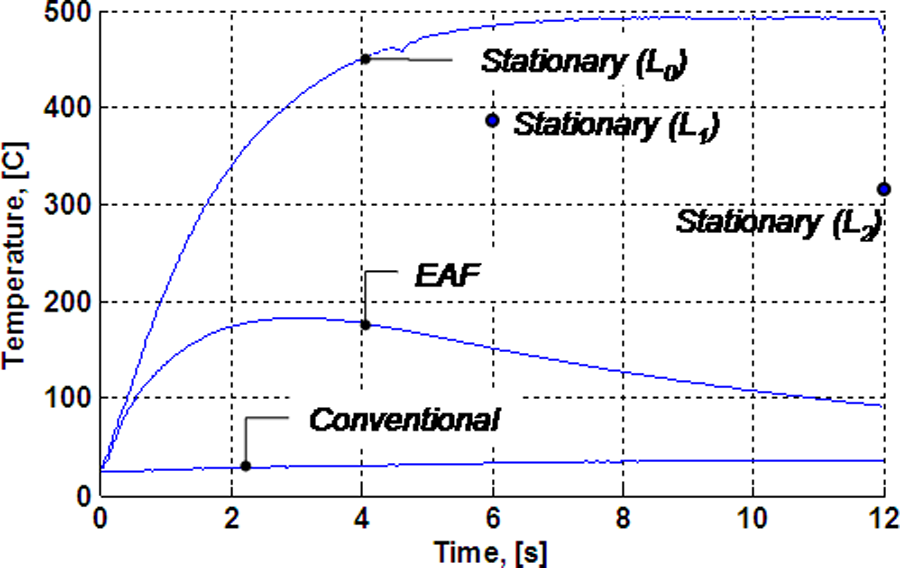
L₀ to L₂ model, EAF, and conversion tests (G2).

After experimentation with different EEC relations, the model and experimental EAF thermal profiles were matched using a power law function to represent the EEC, as shown in Figure 12. The same model prediction process procedure was followed for Ti–G5. The model and experimental results for the stationary test are shown in Figure 13. For this test, a specimen machined to L₂ dimensions was used in the experiments. The model and experiments matched closer than for Ti–G2.

Figure 12.

L₀ to L₂ model with EEC.

Figure 13.

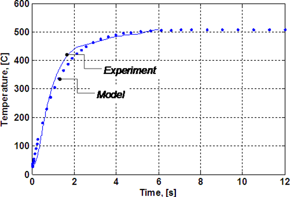
Stationary test at L₂ (G5).

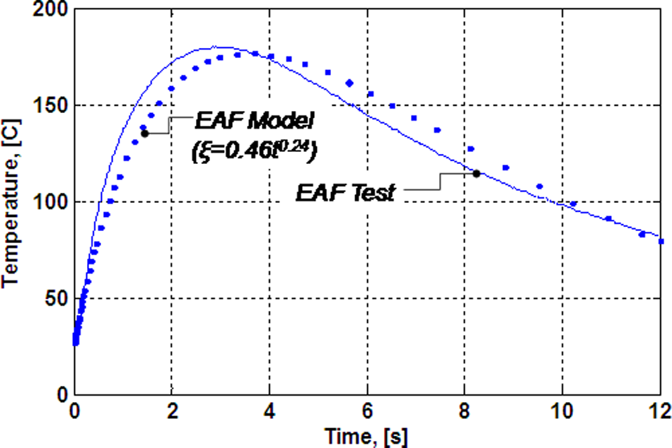
As was done for Ti–G2, an EEC function was developed to match the model and experimental EAF thermal profiles, shown in Figure 14. For this material, the model produced roughly the same peak temperature as the experiments, but the model showed a slightly slower heating profile, as was also seen for Ti–G2.

Figure 14.

L₀ to L₁ EEC profile (G5).

Figure 15 displays the EEC profiles for an EAF test from L₀ to L₂ (0 s to 12 s). Of note is that the Ti–G5 profile ends at 6 s, while the Ti–G2 profile extends to 12 s. This is because the Ti–G5 specimens failed after L₁ and were not able to be conventionally formed to L₂ without fracture. The coefficients were found to be non-linear, and were approximated using the power law, as shown in equation (10)

ξ = ξ_{0} * t^{a}

(10)

where ξ₀ is an initial value, which is dependent on specific material properties and the magnitude of the applied current, t represents time, and a is an exponential term. Although the EEC does not simply vary in time, the term ‘time’ is related to the deformation parameters. Equation (10) can be re-written in terms of strain, as shown in equation (11), where $ε$ is the material strain and $\overset{\cdot}{ε}$ is the strain rate (i.e. the deformation speed). The relationship of a is not clearly understood yet, and more experiments are required to investigate this exponent in more detail.

ξ = ξ_{0} * {(\frac{ε}{\overset{\cdot}{ε}})}^{a}

(11)

Figure 15.

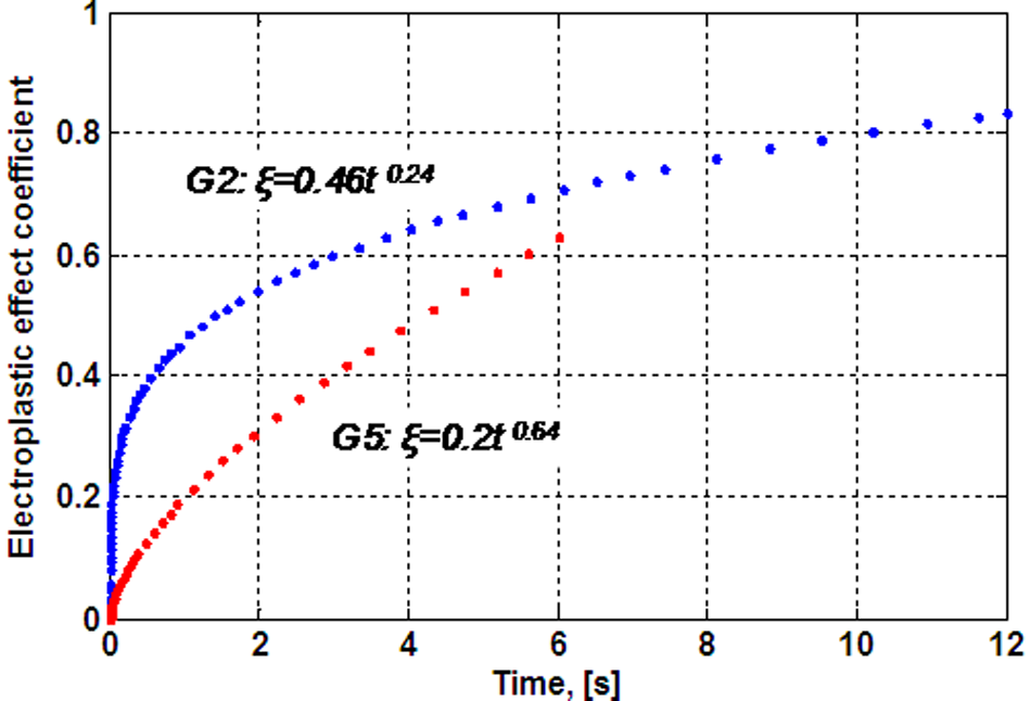
L₀ to L₂ EEC profiles (G2 and G5).

From Figure 14, the EEC for each Ti-grade is different, owing to differences in the electrical, thermal, and microstructure properties of the two materials. Specifically, the Ti–G2 EEC increased rapidly in the first few seconds of deformation, hence the larger ξ₀ value, whereas the Ti–G5 EEC increased more consistently throughout the length of the test, hence the larger a value.

The difference between model predictions and experiments was computed, and the maximum and minimum differences, as compared to the experimental measurements of the temperature, are presented in Figure 16. For most of the tests, the model predicted the temperatures with less than ± 12% error, while one of the tests underestimated some of the values with about –20%. Overall, the model predictions agree well with the measurements, but refinement will be needed for more accuracy.

Figure 16.

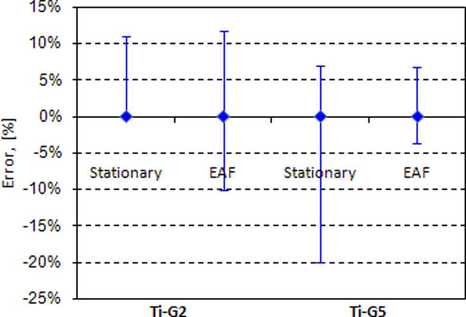
Percent error between the model predictions and experiments.

Effect of prior cold work

Within this sub-section, the effect that prior plastic deformation (i.e. cold work) has on thermal profiles and true stress–strain profiles is discussed. Figure 17 shows the temperature recorded during two stationary tests at L₂, where two different Ti–G2 specimen types were used: one with significant cold work (L₂ deformed) and one without any cold work (L₂ machined). Before running the stationary test, different steps were taken to produce each specimen. For preparation of a cold-worked specimen, a L₀ specimen was compressed to L₂, or a true strain of about 0.57, thus increasing the dislocation density and residual stress state within the material. To produce the non-worked specimen, a combination of centerless grinding and EDM processes were used to replicate the size of a deformed L₂ specimen. When preparing the cold-worked specimen, barreling was not replicated. The cold-worked specimen has a significantly lower thermal profile compared to the work-free machined specimen. The lower thermal profile of the worked specimen can be attributed to the many dislocations and stress fields that the applied electricity could “push” or “relieve”. In doing this, not all of the electricity is contributing to resistive heating. Conversely, in the machined specimen, there are not many dislocations or stress fields that can absorb much of the applied electrical energy. Hence, more of the electricity goes towards resistive heating, which generates the higher thermal profile.

Figure 17.

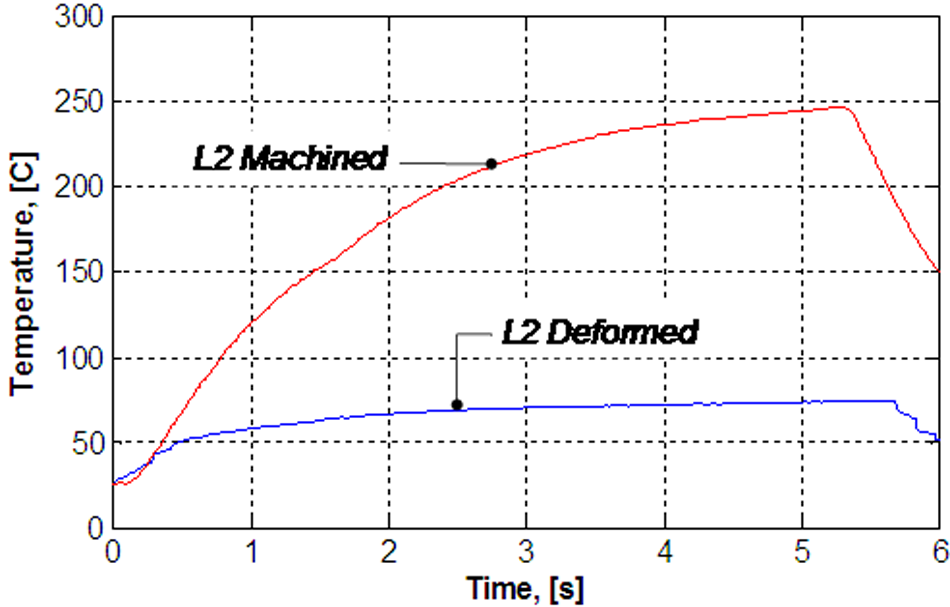
Stationary test at L2 (G2).

Figure 18 displays the effect that prior cold work/EAF have on the true stress–strain profiles of Ti–G2 specimens. The stress–strain profiles are from L₁ to L₂. As was done with the thermal cold-work relationship investigation, specimens were either conventionally formed from L₀ to L₁ (to instill cold work), or they were machined to L₁ size specifications (to produce parts free of cold work). For each specimen type, conventional and EAF tests at 300 A were run. It can be observed that the EAF tests lowered the flow stress for both specimen types. However, for the initially machined specimens that had no cold-work, the reduction in flow stress owing to EAF was over double the flow stress reduction in the initially deformed cold-worked specimens. The minimal flow stress reductions for the initially deformed specimens may be owing to the fact that the applied magnitude of current was unable to mobilize many of the dislocations in the material because the dislocation density in the material lattice was increased significantly from the cold working.

Figure 18.

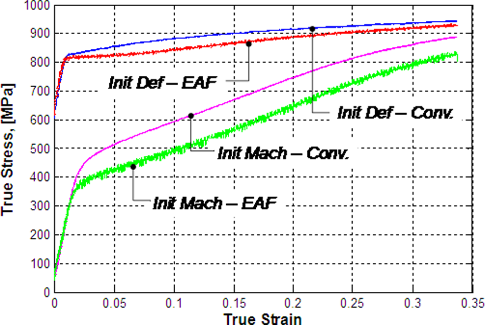
Stress–strain profiles from L1 to L2 (G2).

These results are different from the observations of Siopis et al., which explored the combined effect of grain size and dislocation density on the effectiveness of EAF at the microscale.^14,15 They observed that the stress reduction owing to EAF increased as the grain size decreased and the dislocation density increased. Note that, in the work presented here, since there was not severe deformation, it is not expected that the grain size changes, but rather the effect of dislocations density is separately investigated.

Contact force effect on temperature

Another input variable that can affect EAF thermal profiles is the contact force witnessed between the specimen and the top/bottom dies. Figure 19, shows that, as the contact force is increased the overall temperature of the specimen is decreased. To produce this figure, stationary tests were performed on initially machined (non-worked) specimens at L₂ dimensions with varying contact forces. To reduce variability, a new specimen was used for each test, and the applied force did not exceed the yield strength of Ti–G2 at these dimensions, so plastic deformation did not occur. From the figure, it can be seen that there is a strong inverse relationship between the contact force and specimen temperature. This may be attributed to the lower resistance of the part with increase in load, as the elastic deformation of the asperities of the surfaces in contact results in increased contact area at the dies/specimen interfaces. The thermal model proposed in this work does not currently include a variable for contact force, but future revisions will incorporate it.

Figure 19.

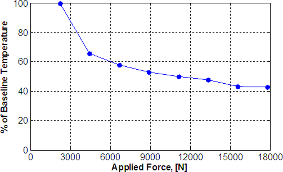
Contact force effect on temperature (G2).

Influence of changes in material properties with temperature

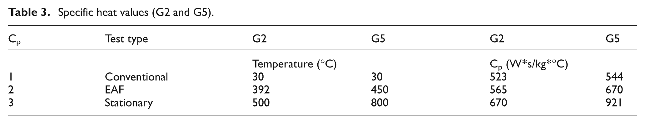
As the temperature of the specimen increases during each test, the material properties have the potential to vary with the temperature increase. Figures 20 and 21 display thermal profiles for stationary tests calculated using different specific heat values for Ti–G2 and Ti–G5, respectively. The selected specific heat values are representative of the temperatures occurring at the particular tests (conventional deformation test, EAF test, and stationary test). These values are summarized in Table 3.²⁰ One can see a noticeable difference in the thermal profiles owing to the changes in the specific heat values from test-to-test for Ti–G5. This was also seen for the Ti–G2 material, but the differences in the thermal profiles were not as large. From the figures, it is clear that the change in specific heat values with temperatures can have a moderate effect on the specimen heating profile, and therefore, a variable specific heat value as a function of temperature should be incorporated into future revisions of the model.

Figure 20.

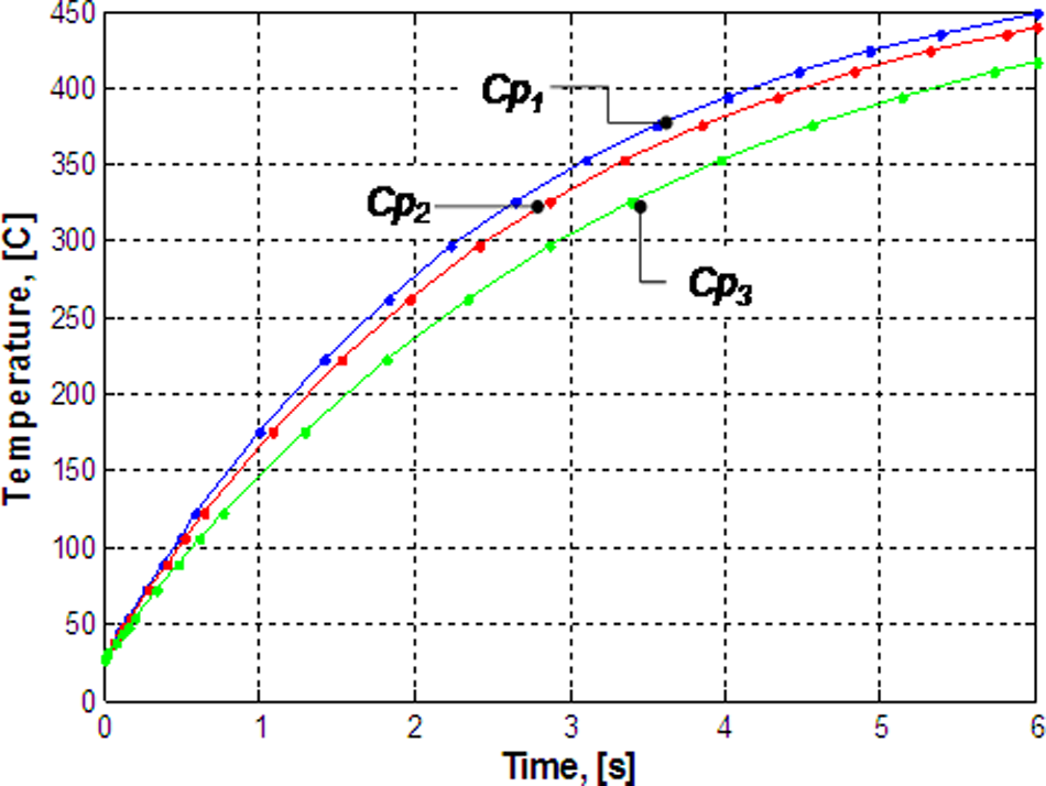
Specific heat effect (G2).

Figure 21.

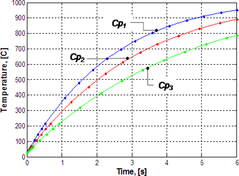
Specific heat effect (G5).

Table 3.

Specific heat values (G2 and G5).

C_p	Test type	G2	G5	G2	G5
		Temperature (°C)		C_p (Ws/kg°C)
1	Conventional	30	30	523	544
2	EAF	392	450	565	670
3	Stationary	500	800	670	921

Conclusions and future work

This paper analyzes the thermo-mechanical aspects of the electroplastic effect. A thermal model, accounting for different forms of heat transfer, material properties specifically for titanium alloys, previous cold work, and various levels of plastic deformation, was verified using experimental EAF tests. Moreover, the effects of varying material properties and contact pressure at the die/workpiece interface were also investigated experimentally. The conclusions from this work are as follows.

EAF reduced the flow stress in both Ti–G2 and Ti–G5. Although just one current was used, 300 A DC, based on previous work, similar results are expected for different currents.

To account for varying differences in thermal profiles between the conventional/EAF tests, a new EEC was introduced, which was defined by a power law relation.

The EECs for the two Ti-grades were significantly different. This is because the grades of titanium were different. Ti–G2 is a single-phase polycrystalline material, and Ti–G5 is a dual-phase alpha–beta alloy. For Ti–G2, the electrons were able to travel easier because they only had to move through one phase. This can be seen by noticing the steeper and higher EEC for Ti–G2 compared to Ti–G5.

The effect of prior cold work was notable to both the thermal and stress–strain profiles of the Ti.

Contact force had a strong, but inverse relationship with specimen temperature.

The variation in the specific heat of the materials had a small effect on the thermal profiles.

Future work will first include integration of the variable EEC in the thermo-mechanical model for prediction of the stress–strain relationship during EAF compression tests. Next, the effects of previous cold work and contact pressure will be incorporated into the thermal model. Additionally, the model can be expanded to other materials, by simply modifying the material properties, specimen dimensions, and test parameters. Further, tribological modeling, where asperity crushing is modeled, will need to be performed since the real contact area has a notable effect on the overall thermal profile of the workpiece. Moreover, the fundamental understanding of electroplastic effects can be potentially extended to various other EAF and EAM processes.

Footnotes

Appendix

Acknowledgements

The authors would like to acknowledge Ionic Technologies Inc. for heat treating the EAM-compression dies, and Insulfab Plastics Inc. for providing insulation material used in the dies.

This research received no specific grant from any funding agency in the public, commercial, or not-for-profit sectors

References

Salandro

Roth

. Electrically-assisted manufacturing. In: Zhang

(ed) Intelligent EFM and interdisciplinary process innovations. CRC Press, 2010, pp. 505–536.

Bunget

Salandro

Mears

. Energy-based modeling of an electrically-assisted forging process. Transactions of the North American Manufacturing Research Institute of SME 2010; 38.

Machlin

. (1959). Applied voltage and the plastic properties of “brittle” rock salt. J Appl Phys 1959; 30(7): 1109–1110.

Nabarro

FRN

. Theory of crystal dislocations, Chapter IX, 1967.

Troitskii

. Electromechanical effect in metals. Pis’ma Zhurn Experim Teoret Fiz 1969; 10: 18.

Okazaki

Kagawa

Conrad

. A study of the electoplastic effect in metals. Scripta Metallurgica 1978; 12(1): 1063–1068.

Klimov

Novikov

. The “Electroplastic Effect”. A.A. Baikov Institute of Metallurgy, Acad. of Sci. of the USSR, Moscow. Trans. from Problemy Prochnosti 1982; 2: 98–103.

Lai

Chen

. Effect of electric current on the recrystallization behavior of cold worked alpha-Ti. Scripta Metallurgica 1988; 22: 187–190.

Chen

Liu

. Electric current effects upon the Sn/Cu and Sn/Ni interfacial reactions. J Electronic Mat 1998; 27: 1193.

10.

Conrad

. Thermally activated plastic flow of metals and ceramics with an electric field or current. Mat Sci & Engr 2002; A322: 100–107.

11.

Andrawes

Kronenberger

Roth

. Effects of DC current on the mechanical behavior of AlMg1SiCu. Mat Mf Proc 2007: 22(1); 91–101.

12.

Perkins

Kronenberger

Roth

. Metallic forging using electrical flow as an alternative to warm/hot working. J Mf Sci Engng 2007; 129(1): 84–94.

13.

Ross

Irvin

Roth

. Manufacturing aspects relating to the effects of DC current on the tensile properties of metals. J Engr Mat Tech 2007; 129(2): 342–347.

14.

Siopis

Kinsey

Kota

. Effect of severe prior deformation on electrical-assisted compression of copper specimens. In: International Manufacturing Science & Engineering Conference, 2010, MSEC2010-34276, pp. 7.

15.

Siopis

Kinsey

. Experimental investigation of grain and specimen size effects during electrical-assisted forming. In: International Manufacturing Science & Engineering Conference, 2009, MSEC2009-84137, pp. 6.

16.

Dzialo

Siopis

Kinsey

. Effect of current density and zinc content during electrical-assisted forming of copper alloys. CIRP Annals – Mfg Technol 2010; 59(1): 299–302.

17.

Kronenberger

Johnson

Roth

. Coupled multifield finite element analysis model of upsetting under an applied direct current. J Mfg Sci Engng 2009; 131.

18.

Ross

Kronenberger

Roth

. Effect of DC on the formability of Ti-6AL-4V. J Engng Mat Technol 2009; 131(3): 11.

19.

Salandro

Bunget

Mears

. Electroplastic modeling of bending stainless steel sheet metal using energy methods. International Manufacturing Science & Engineering Conference, 2010, MSEC2010-34043, pp. 10.

20.

United States Department of Defense (2003). Department of Defense Handbook: Metallic materials and elements for aerospace vehicle structures, MIL-HDBK-5J.

A thermal-based approach for determining electroplastic characteristics

Abstract

Keywords

Introduction

Lightweight manufacturing in automobiles

EAM

Development of EAM

Objective and approach

Methodology

Aspects of the electroplastic effect

Assumptions of the thermal model

Development of the thermal analytical model

Experimental set-up and procedure

Results and discussion

Force reduction owing to EAF

Model prediction and experiments

Effect of prior cold work

Contact force effect on temperature

Influence of changes in material properties with temperature

Conclusions and future work

Footnotes

Appendix

Acknowledgements

References