Sage Journals: Discover world-class research

Abstract

The use of individual-level browsing data, that is, the records of a person’s visits to online content through a desktop or mobile browser, is of increasing importance for social scientists. Browsing data have characteristics that raise many questions for statistical analysis, yet to date, little hands-on guidance on how to handle them exists. Reviewing extant research, and exploring data sets collected by our four research teams spanning seven countries and several years, with over 14,000 participants and 360 million web visits, we derive recommendations along four steps: preprocessing the raw data; filtering out observations; classifying web visits; and modelling browsing behavior. The recommendations we formulate aim to foster best practices in the field, which so far has paid little attention to justifying the many decisions researchers need to take when analyzing web browsing data.

Keywords

web browsing data digital trace data web tracking data computational social science

Digital traces—data that emerge from people’s interactions with digital systems (Howison et al., 2011)—are an increasingly valuable scientific resource. A subset of trace data concerns people’s activity when seeking out and consuming online information—so-called web browsing or web tracking data. Researchers use such data to explore a wide variety of phenomena across the social sciences, from ideological polarization (Gentzkow & Shapiro, 2011) and selective news exposure (Nelson & Webster, 2017) to online shopping (Santos et al., 2012) and porn consumption (von Andrian-Werburg et al., 2023). Browsing data hold great potential, especially when linked with surveys (Stier, Breuer, et al., 2020), but their characteristics also raise statistical questions less common for traditional data sources.

There is some literature conceptualizing trace data in general (Keusch & Kreuter, 2021) as well as measurement frameworks for browsing data in particular (Bosch & Revilla, 2022b). Scholars have also worked on the challenges of collecting browsing data such as user privacy (Menchen-Trevino & Karr, 2022; Silber et al., 2022) and reviewed the growing number of collection tools (Christner et al., 2022). Our question is different: How should browsing data be handled once collected? To our knowledge, there is no guide for avoiding the pitfalls of browsing data while harvesting their enormous potential.

We structure our recommendations along four steps. First, researchers have to make many decisions when preprocessing raw variables. For example, what is the correct way to extract domains from URLs? Second, browsing data are inherently messy, and researchers may consider filtering out observations such as duplicated visits. Third, researchers often wish to classify large quantities of browsing into more manageable categories, which can be done in many different ways. Last, modelling browsing behavior raises thorny questions, for example, regarding statistical power in panel models.

We review the choices made in previous studies and derive recommendations from exploring our own ten data sets, which span seven countries (France, Germany, the Netherlands, Poland, Spain, the UK, and the U.S.), were collected between 2015 to 2022, with a total over 14,000 participants recruited by six different panel providers (Kantar, Lucid, Netquest, Panel Ariadna, Respondi, and YouGov), and comprise more than 360 million web visits. This wide coverage ensures that our advice is not based on idiosyncrasies of any one data set but is applicable to research at large. We use our data to describe typical properties of browsing data and to test the sensitivity of results to analytical decisions. Our final contribution is a hands-on code guide (SM B, also published at https://bernhardclemm.com/browsing-data-code-guide/index.html), which implements the described analytical steps (in R and SQL). This will allow scholars unfamiliar with browsing data to enter this exciting field easily.

(Our) Browsing Data

We focus on individual-level browsing data, defined as the records of a person’s visits to online content through a desktop or mobile browser (or apps). These data have—in general—at least three variables: a URL, a timestamp, and a participant identifier (Figure 1).

Figure 1.

A typical web browsing data set. “id” is the participant identifier; “timestamp” is the time of the visit; “url” is the URL of the visit.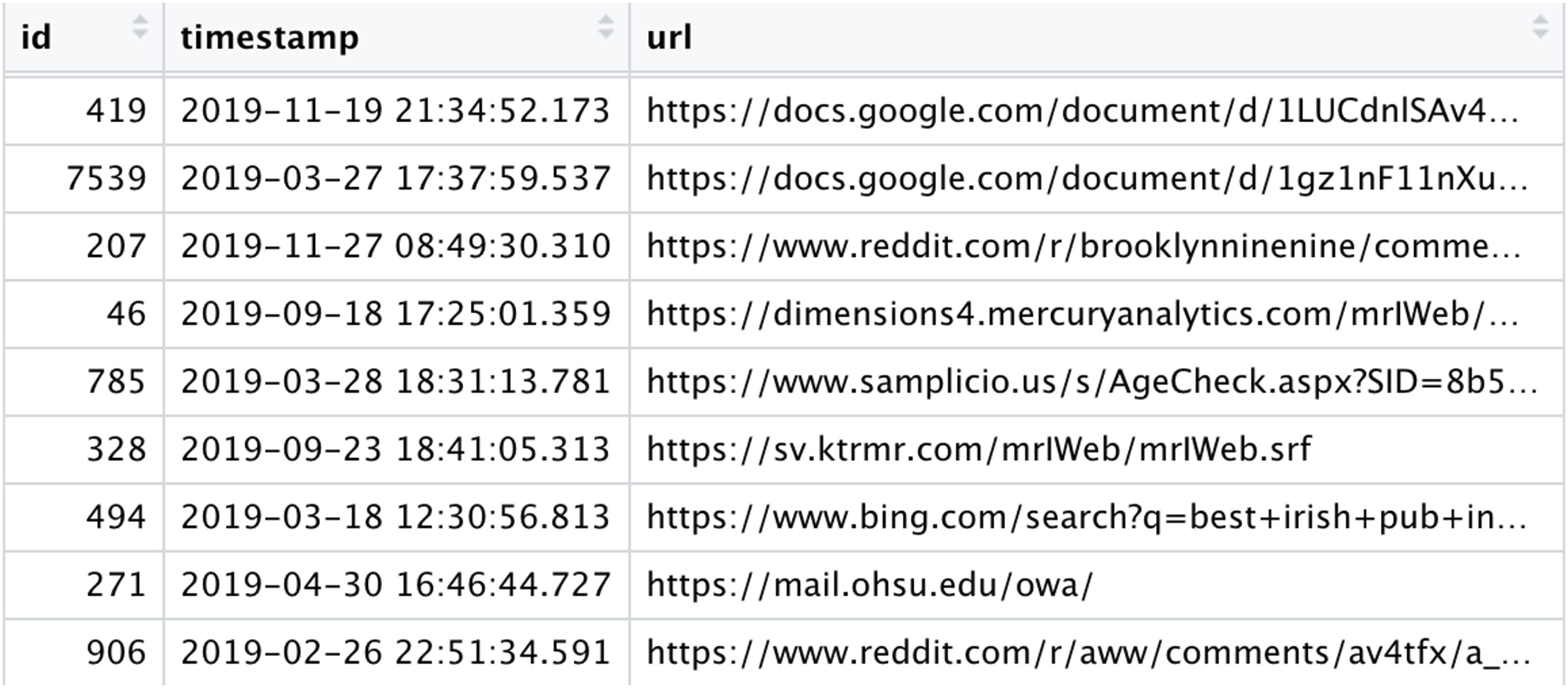

There are exceptions to this typical version of web browsing data. Variables may be more limited: For example, some data vendors only provide a web domain, not the URL. App usage data does not include a URL, but an “app name” variable. In other cases, more variables are available: Some tools provide a measure of visit duration (which can also be approximated with timestamps, cf. Section “Defining visit duration”) or the “title” of a website (cf. Section “Classifying by website titles or paths”). More recent technologies collect the HTML of visited pages (Adam et al., 2023). The different levels of data “richness” have implications for classification purposes (cf. Section “Classifying browsing data”).

The ten browsing data sets we explore, all paired with survey data, follow this basic structure, with slight differences in terms of the variables (Table 1). Our data sets vary on a number of important dimensions, one of which is the tool with which browsing data were collected, the key distinction being between “donated-data” and “tracked-data” technologies.

Table 1.

Overview of Data Sets.

Time	Country	Collection technology	Provider	Devices	Waves	# Subjects^a	# Visits (m)
2015	USA	Wakoopa^b	YouGov	Desk	1	1392	6.3
2018–2019	GER	Wakoopa^b,c	Respondi	desk.+mob	3	3074	93.8
2019–2020	NED	WebHistorian^d,f	Kantar	Desk	3	3027	56.8
2019–2020	POL	WebHistorian^d,f	Panel Ariadna	Desk	3	2076	49.2
2019–2020	USA	WebHistorian^d,f	Lucid	Desk	3	2392	129.8
2022	ESP	Wakoopa^b	Netquest	desk.+mob	2	366	6.6
2022	FRA	RealityMine^b,e	YouGov	Desk	2	359	6.4
2022	GBR	RealityMine^b,e	YouGov	desk.+mob	2	410	4.5
2022	GER	RealityMine^b,e	YouGov	desk.+mob	2	355	6.6
2022	USA	RealityMine^b,e	YouGov	desk.+mob	2	443	7.1

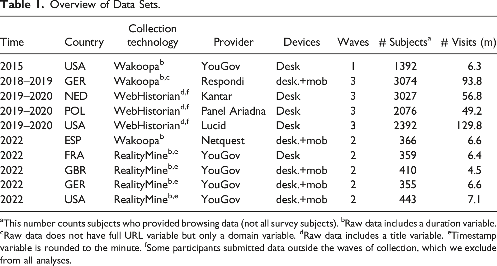
^aThis number counts subjects who provided browsing data (not all survey subjects). ^bRaw data includes a duration variable. ^cRaw data does not have full URL variable but only a domain variable. ^dRaw data includes a title variable. ^eTimestamp variable is rounded to the minute. ^fSome participants submitted data outside the waves of collection, which we exclude from all analyses.

The open-source WebHistorian tool follows a donated-data paradigm and collects users’ visit history stored in their browsers. Participants submit their data ex post, and browsing is not recorded continuously (cf. Menchen-Trevino, 2016). In a tracked-data approach (Wakoopa and RealityMine), participants install tracking software on their device(s). Tracked data are commonly collected by commercial companies. A benefit of donated-data solutions is that they require no longer-term commitment by participants and may avoid Hawthorne effects. However, donated-data solutions typically work for desktop only, whereas tracking technologies cover multiple devices and mobile apps.

To explore the sensitivity to analytical decisions, we focus on exposure to news and to social media as exemplary variables throughout the paper. This is not because our recommendations are restricted to these topics but because they were accessible across data sets. We are confident our recommendations will travel to other research topics—for example, online shopping (Santos et al., 2012) or use of health-related information (Bachl et al., 2023).

Preprocessing Browsing Data

Parsing URLs

The URL is the key to classifying web browsing into useful categories. Parsing URLs requires a thorough understanding of their anatomy, which we illustrate in Figure 2. For research purposes, the most relevant parts are the host, the domain, the path, and the query with its parameters. A variety of packages such as adaR (R) (Schoch & Chan, 2023), webtrackR (R) (Schoch et al., 2023), urltools (R) (Keyes et al., 2019), or tld (Python) (Barseghyan, 2013) provide functions for parsing these components, which we discuss below. In SM A.1.4, we additionally discuss how to process “app names” that emerge from app usage data.

Figure 2.

Structure of a fictitious URL. We ignore other components (such as port or username) less relevant for researchers. Italicized terms are used ambiguously, as discussed below.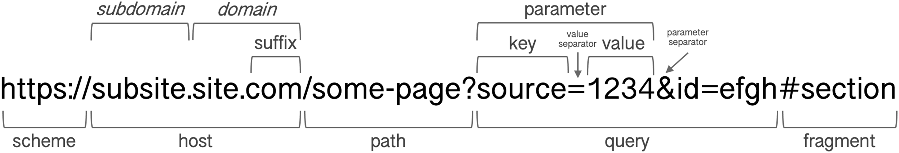

Extracting Hosts and Domains

Both domain and host are useful starting points to categorize browsing behavior. For example, to measure shopping activity, one could compile a list of e-commerce domains such as “amazon.com” and “ebay.com.” A host always includes the domain but sometimes additionally contains a subdomain and can thus be more informative. For example, “music.amazon.com” reveals more about the visit than just “amazon.com.”

In contrast to the host—the part between the scheme and the path—the term “domain” does not have a strict technical definition. We use it in the common colloquial meaning: the part of a URL that identifies the person or organization in control of the site. In technical terms, we mean the top domain under a registry suffix, that is, the rightmost part of the URL before, and including the registry suffix, which is the “ending” under which one can register a domain. Not all (though most) suffixes are registry suffixes, which adds complexity to the definition and extraction of domains, as we elaborate in SM A.1.1.

Some data vendors include a pre-measured domain variable in the data. Otherwise, the domain needs to be extracted. Looking at Figure 2, this seems deceptively straightforward: Extract the host and split it at each dot; the domain consists of the last two parts. However, as the suffix structure and the number of dots are not standardized, such rules of thumbs do not work. Domain extraction must be based on the Public Suffix List (PSL), a list of all suffixed maintained by the Mozilla Foundation (2022) and used by common URL parsing packages. In SM A.1.2, we test how well common R packages extract domains.

Even when a domain variable is pre-measured by data vendors, it is worthwhile to compare it to the domain extracted with open-source packages. As shown in Table 2, the extracted and pre-measured domains are identical most of the time, but not always. We discuss different cases of non-correspondence in SM A.1.3. Given these possible discrepancies, we suggest researchers rely on their own extraction rather than on a variable provided by commercial vendors. We provide code for domain extraction in SM B.2.1.

Table 2.

Percent of Visits for Which the Domain Pre-measured by the Data Vendor and the Domain Extracted With adaR Correspond. Only Data Sets With a Pre-measured Domain Included.

Data set	% Correspondence
2015-USA-Wakoopa	99.9
2022-ESP-Wakoopa	99.2
2022-FRA-RealityMine	95.9
2022-GBR-RealityMine	96.0
2022-GER-RealityMine	97.3
2022-USA-RealityMine	96.6

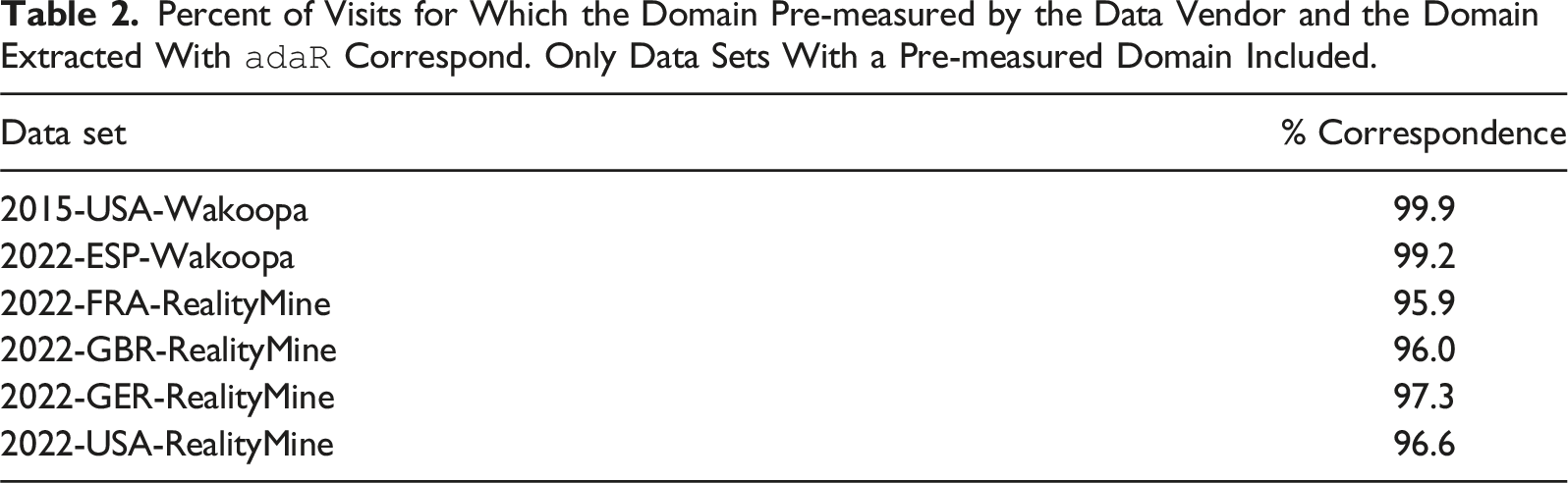
Recommendation #1: Parse URLs with open-source packages rather than relying on variables by data providers.

Extracting Paths and Queries

The extraction of paths and query strings is more straightforward and can be done with most parsing packages (code in SM B.2.1). The path is an interesting data point in itself, as it often provides a clue about the page content. For example, researchers studying news content might extract the path of the URL “https://www.theguardian.com/politics/2023/aug/01/boris-johnson-swimming-pool-newts-oxfordshire,” namely, “boris johnson swimming pool newts oxfordshire,” and use it as an input for classification (cf. Section “Classifying by website titles or paths”).

The query string opens the door to several important variables. First, it can be used to identify referrals (cf. Section “Defining referrals”). Second, search engines typically include a user’s search into the query string, for example, a Google search will appear in the URL as “search = [search terms].” Scholars have made fruitful use of such search parameters, for example, to test the impact of the search engine rankings (Ulloa & Kacperski, 2023) or to explore searches related to politics (Menchen-Trevino et al., 2023) or health (Bachl et al., 2023).

Defining Visit Duration

In their barest form, web browsing data reveal when a user visited a certain URL—but not for how long. Yet, from a theoretical perspective, the duration of visits is just as relevant as their number. Conceptualizing the duration of a visit is in itself not simple. Consider a user who opens a web page, reads it for 1 minute, and then looks out the window for 2 minutes before closing the page. Is this is a visit of 1 or 3 minutes? Beyond conceptualization, there is no way for any tool to measure such subtleties.

Most tracking tools provide a duration variable—though the exact operationalization is a black box, and we tried in vain to get a precise explanation of its measurement from one panel provider. Nevertheless, many studies, including some of our own, rely on the tracker-provided duration variable (e.g., Aslett et al., 2022; Cardenal et al., 2019; Guess, 2021; Nelson & Webster, 2017; Scharkow et al., 2020; Stier et al., 2022). When browsing data do not contain a duration measure, it can be approximated via timestamps. The simplest approach entails setting the duration of a visit to the difference between its timestamp and the timestamp of the next visit, using some cutoff when this difference is large (e.g., Casas et al., 2022; Wojcieszak, Menchen-Trevino, et al., 2023; code for implementation in B.2.2).

In this approach, the choice of the cutoff and of a replacement value when the cutoff is exceeded are crucial. To shed light on optimal choices, for three data sets, we compared how well the pre-measured duration (which we use as a benchmark) correlates with a timestamp-based approximation, varying cutoff and replacement values (see SM A.2). The results show, first, that optimal cutoffs tend to be low, usually below or around 5 minutes. Second, correlations are generally highest if timestamp differences above the cutoff are set to missing. Note that this approach will create missing data, which may be problematic for certain aggregations. The second-best replacement value is the cutoff value. These analyses can serve as a rough orientation; we hope that future tracking solutions provided by academics will provide more transparent duration measurements.

Recommendation #2: When approximating duration with timestamps, choose a cutoff of below or around 5 minutes and set differences exceeding this cutoff to missing (if the resulting missing data does not create further problems).

Defining Referrals

Given the central role of online intermediaries—platforms like Facebook, Google, or Twitter—in the digital ecosystem, researchers have started to investigate the role of the so-called “referrals” from these platforms, that is, users following links to outside content (Cardenal et al., 2019; Guess, Nyhan, & Reifler, 2020; Möller et al., 2020; Stier et al., 2022; Wojcieszak et al., 2021). Since most collection tools do not capture behavior within online platforms, we can only indirectly infer which visits were triggered by referrals.

The most common approach is to simply order browsing histories sequentially and define a visit preceded by a platform visit as a referral. For Facebook-referred visits alone, a recent study identified three variants of this approach (Schmidt et al., 2023). A fourth approach infers referrals from the URL parameter “fbclid” contained in the query string. The study validated each approach by applying it to data from a tracking tool that also captures the HTML of public Facebook posts seen by participants (Adam et al., 2023). This direct observation of whether a visit was Facebook-referred was used as a benchmark for validation, showing that many of the referrals identified are false positives (up to 43%). Sequence-based approaches overestimate referrals as they implausibly assume that any visit after a Facebook visit is caused by clicking on a link in Facebook.

Better results—with up to 90% accuracy—are achieved by inferring referrals from the URL parameter “fbclid,” a pattern directly observable in browsing data (Schmidt et al., 2023; see SM B.2.3 for code). Although we are not aware of research testing the reliability of parameters for other platforms, the available evidence suggests that defining referrals based on URL parameters, rather than timelines, is the most valid approach.

Recommendation #3: When defining platform referrals, try to find relevant URL parameters that indicate that a visit was referred.

Filtering Browsing Data

Missing Visits

With browsing data, missing data can be hard to recognize, since it is not always clear what “complete” data look like. As shown in Table 3 and detailed in SM A.3, some participants have little, or at least less than the maximum, activity across the study period. Existing studies typically do not discuss the possibility of missing data in detail. If anything, researchers drop participants with few data points. For example, Cronin et al. (2022) exclude participants with fewer than seven days of data and Fletcher et al. (2021) drop subjects with fewer than five news visits.

Table 3.

Patterns of Participants’ Data Availability. “Days” Refer to Any Day That the Subject Provided Data. For Multi-Wave Data Sets, Only One Wave is Summarized.

Data set	% with <7 days	Maximum n of days	Median n of days
2015-USA-Wakoopa	31.18	21	10
2018-GER-Wakoopa	9.71	74	41
2019-NED-WebHistorian	5.65	92	60
2019-POL-WebHistorian	6.31	92	49
2019-USA-WebHistorian	3.89	92	62
2022-ESP-Wakoopa	9.76	84	58.5
2022-FRA-RealityMine	4.41	89	67
2022-GBR-RealityMine	7.98	89	74
2022-GER-RealityMine	8.24	88	69
2022-USA-RealityMine	5.44	74	66

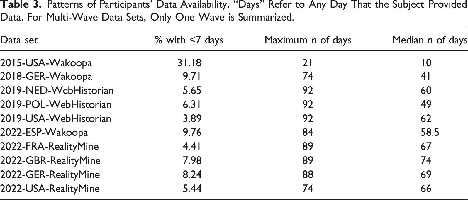
Who are the participants with little data? We distinguish two cases: First, participants may simply spend little time online, in which case the data are not missing. Second, data collection may truly have missed some browsing behavior. Participants may navigate the Internet on devices the study does not track, or interfere with the collection technology, by periodically deleting their data (in the case of donated data) or by temporarily disabling the tracker (as they are allowed to by most tracked-data providers).

Is there any way to distinguish missingness from true low browsing frequencies? One indication may be temporal concentrations of active days. Figure 3 contrasts two cases from our donated-data samples. Panel A shows a subject with consistently few visits across time. In contrast, Panel B shows a participant who provided data almost every day for a very short period immediately before data submission. Most likely, this participant cleaned their browsing history shortly before submission. SM B.3.1 provides code for detecting such patterns.

Figure 3.

Two subjects with small data quantities (from 2019-NED-WebHistorian and 2019-POL-WebHistorian). Dashed lines indicate day of data submission.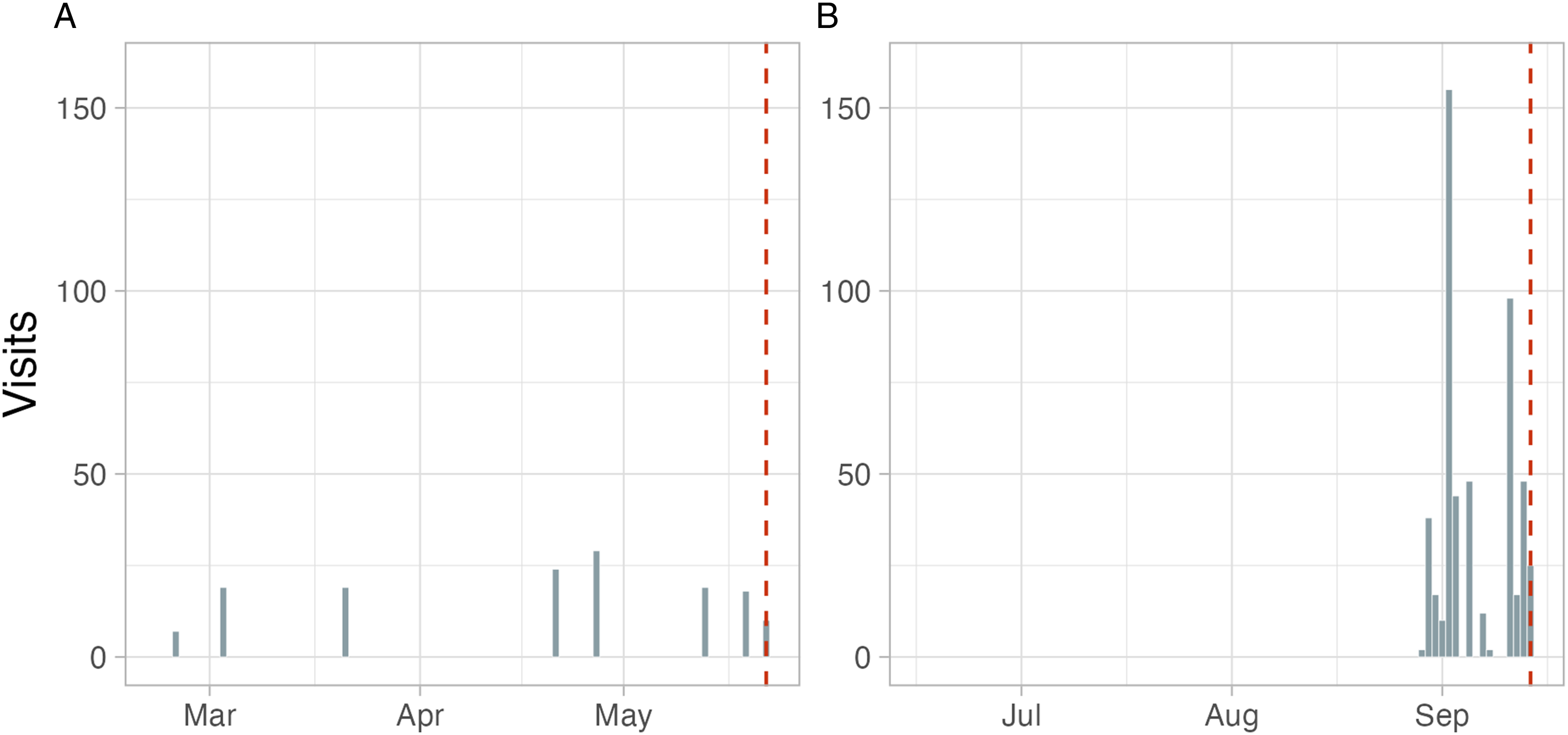

To approach the issue of missing data systematically, we recommend classifying the missingness process according to Rubin’s categories: missing completely at random (MCAR), missing at random (MAR), or not missing at random (NMAR). MCAR assumes a process in which missing and observed data are drawn from the same distribution, a condition not likely to hold in general. Less restrictively, MAR assumes an equal probability of missingness conditional on some observed covariates (such as use of a mobile versus desktop device). NMAR might be relevant if, for example, some visits were not recorded due to a technical issue unrelated to participant characteristics.

Researchers can use established tests (e.g., Little & Rubin, 2019) in order to assess whether MCAR holds. If it does, researchers may drop participants with missing observations. In the case of temporal clustering as exhibited in Figure 3B, the researcher may have to accept NMAR, which forecloses many of the solutions offered in the missing-data literature. Typical recommended approaches in this situation include conducting sensitivity analyses under different assumptions about the sources of missingness.

If MAR is plausible, missing observations can be imputed. Most likely, this will not be done for individual visits, but rather classes of visits (e.g., visits to shopping sites). The specific technique will likely depend on whether the browsing data will be used as an outcome or as a predictor. In the former case, multilevel imputation is a promising solution (Van Buuren, 2018). Substantial literature on multilevel imputation discussed applications to longitudinal data (e.g., Fitzmaurice et al., 2008). If browsing data will be used as a predictor, recent developments in econometrics suggest methods for imputation in high-dimensional panel data (Cahan et al., 2023).

Recommendation #4: Test for temporal concentrations of individual data availability to find indications of missingness. Depending on the application, use multilevel or factor-based imputation of missing values.

Duplicated Visits

Sometimes an observed visit might not be “real” but the outcome of an artifact. One common case is duplication: Some websites automatically create multiple visits to the same page within a short time period or auto-refresh after a certain time period. Visits as they appear in the data can also be the product of decisions by data providers, as some providers turn a visit to a URL into two visits after a certain time (Bosch & Revilla, 2022a).

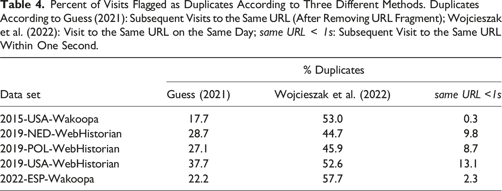
Previous studies have attempted to identify duplicates or similar artifacts and removed them but generally do not offer much justification for their choices (including some of our own work). Guess (2021) defines duplicates as sequential visits to the same URL, after removing the URL’s fragment (also Guess, Nyhan, & Reifler, 2020). Others treat visits to the same URL within the same day as duplicates (e.g., Cronin et al., 2022; Wojcieszak et al., 2022). Kalogeropoulos et al. (2019) check that visits do not constitute page refreshments without mentioning how.

We explore to what extent such choices matter, by measuring the percentage of visits that would be flagged as duplicates in our data sets according to the abovementioned methods by Guess (2021) and Wojcieszak et al. (2022). We add a third method that flags any subsequent visit to the same URL that happens within one second. Arguably, this more conservative method is better justified theoretically: if one assumes that people do not actively reload the same URL within one second, there is a good reason to consider such a visit an artefact. Table 4 shows how widely the occurrence of duplicates varies across methods.

Table 4.

Percent of Visits Flagged as Duplicates According to Three Different Methods. Duplicates According to Guess (2021): Subsequent Visits to the Same URL (After Removing URL Fragment); Wojcieszak et al. (2022): Visit to the Same URL on the Same Day; same URL $<$ 1s: Subsequent Visit to the Same URL Within One Second.

Data set	% Duplicates
Data set	Guess (2021)	Wojcieszak et al. (2022)	same URL <1s
2015-USA-Wakoopa	17.7	53.0	0.3
2019-NED-WebHistorian	28.7	44.7	9.8
2019-POL-WebHistorian	27.1	45.9	8.7
2019-USA-WebHistorian	37.7	52.6	13.1
2022-ESP-Wakoopa	22.2	57.7	2.3

Do these different deduplication methods affect substantive findings? Assume we wanted to compare the use of different social media platforms, measured as a proportion of all visits in the whole data set. Figure 4 illustrates that, although overall tendencies are similar across methods, small differences appear: For example, in the 2015-USA-Wakoopa data, estimates of Facebook use range from 6.6% to 8.8% across methods. In the 2022-ESP-Wakoopa data, one could conclude that subjects use Facebook three times as much as Twitter, or 1.5 times as much, depending on the method.

Figure 4.

Prevalence of exposure to Facebook, Reddit, Twitter, and YouTube (percentage of visits to the respective domain out of all visits) after different deduplication methods. Duplicates according to Guess, (2021): Subsequent visits to the same URL (after removing URL fragment); Wojcieszak et al. (2022): Visit to the same URL on the same day; same URL 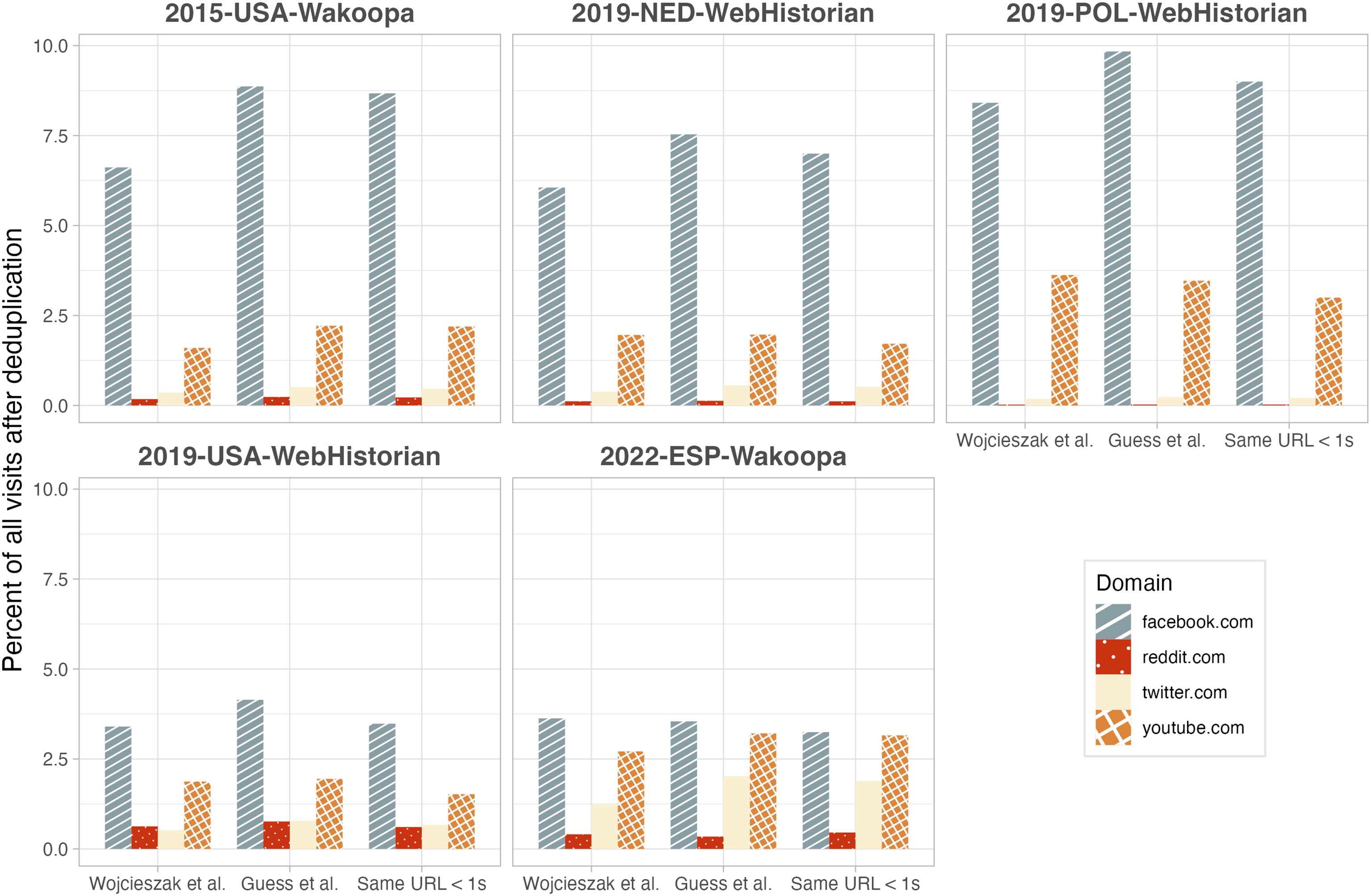$<$ 1s: Subsequent visit to the same URL within one second.

As always, researchers will have to decide whether such differences matter and which operational definition is most justifiable given their study goal. Studies mostly interested in the duration rather than the number of visits can be more relaxed about the issue of duplication: Ten one-second subsequent visits to the same URL can be aggregated to 10 seconds of exposure (Stier et al., 2022). SM B.3.2 provides code for implementation.

Recommendation #5: Depending on your research question, consider excluding duplicate visits.

Incentivized Visits

Another issue that concerns the “realness” of visits is the fact that by design, participants of web tracking studies spend at least some of their time doing surveys for money. As has been shown in one of our papers, the amount of survey taking can be substantive, constituting up to 50% of visits (Clemm von Hohenberg et al., 2024). An open-source list of survey sites compiled for this study can be found on OSF and is applied in SM B.3.3.

What is more, even some visits that seem genuine turn out to be, upon closer inspection, paid visits. There are numerous “get-paid-to” sites that reward people for clicking on or visiting, for example, news sites. As we found in another project, platforms such as “yahoo.com” get a substantive part of their traffic through such schemes. It is possible that such click flows exist in other areas such as shopping.

In both cases, researchers need to think carefully to what extent including survey-taking or incentivized visits may threaten inference. Purely descriptive estimates based on overall browsing quantities will obviously be affected by a high prevalence of such visits—although one could argue that these constitute a working activity just like any other and should not be discarded. The issue may be less relevant for research using a certain browsing behavior as a dependent or independent variable in a model.

Recommendation #6: Depending on your research question, consider excluding survey-taking or incentivized visits.

Classifying Browsing Data

Researchers analyzing web browsing data are typically interested in what kind of content was visited. URLs provide clues about the visited content in several ways. At the highest level, content can be classified via domains, for example, a visit to “facebook.com” as a social media visit. The subdomain or the path of a URL may allow more fine-grained classification, for example, a visit to “facebook.com/theguardian/” could count as news consumption on social media. URLs are also the key to scraping the page content (if HTML is not directly collected by the tracking tool, Adam et al., 2023).

A General Caveat

Although trace data are often heralded as a way to overcome biased survey self-reports, they are vulnerable to many sources of measurement error, as detailed in Bosch and Revilla (2022b). Below, we only touch upon measurement issues at the stage of classification, but researchers should be aware of potential error sources beyond that: Error can emerge, for example, when the target behavior also occurs offline or on other devices, or when the technology fails to capture some browsing (Toth & Trifonova, 2021).

Classifying by Domains (or Hosts)

The most common level for classifying web visits is the domain. Sometimes, the target concept is represented by a single domain. For example, to quantify Facebook use one would simply count visits to “facebook.com.” More often, a behavior of interest is captured by a larger set of websites. There are at least two ways to define such sets.

Open-Source or Custom-Made Lists

One approach is to create new or use existing lists. To compile a list, browsing data can be used inductively, by manually coding the top visited domains in the data for the category of interest. For example, in one of our projects, we coded the 5,000 most visited domains for whether they were news sites (Stier, Kirkizh, et al., 2020, list on OSF). Alternatively, one can rely on audience meter data such as Comscore, which lists the most popular domains of a category. These approaches can be combined: One of our teams compiled over 5,400 U.S. news domains by combining manual coding of the top domains in the data, Alexa audience data, and existing lists of media organizations (Wojcieszak, Menchen-Trevino, et al., 2023, list on GitHub). There is no shortage of open-source lists for a variety of categories, some of which we introduce in SM B.4.1.

As it is impossible to identify all domains associated with a certain browsing behavior, how exhaustive should lists be? Completeness can help to avoid under-coverage (Bosch & Revilla, 2022a) but also requires more work. To explore this trade-off, we match visits in our three U.S. data sets to two different lists of news domains: a “long” one (collected for 2019-USA-WebHistorian) containing 5,400 sites and a “short” one (collected for 2022-USA-RealityMine) with 108 sites. Both combine the most popular domains according to Comscore/Alexa and manually coded top domains in the data.

Figure 5A compares the individual-level counts of news visits based on the two lists. The shorter list tends to under-estimate individual news exposure compared to the longer list. The correlation between the two measures is high for the data set for which the short list was developed (r = 0.82) but low for the data for which the long list was developed (r = 0.17). Figure 5B illustrates that the choice matters on the aggregate level, too: One would estimate the prevalence of news consumption at either below 0.5% or above 2%, depending on the list.

Figure 5.

Comparison between list of news domains. For each of three data sets, we classify visits as news or not based on a “short” and “long” news list. Panel A plots the individual-level counts based on these two lists against each other (excluding outliers beyond the 99-percentile) and reports Pearson’s correlation coefficient. Panel B plots the percentage of news visits out of all visits based on the two methods.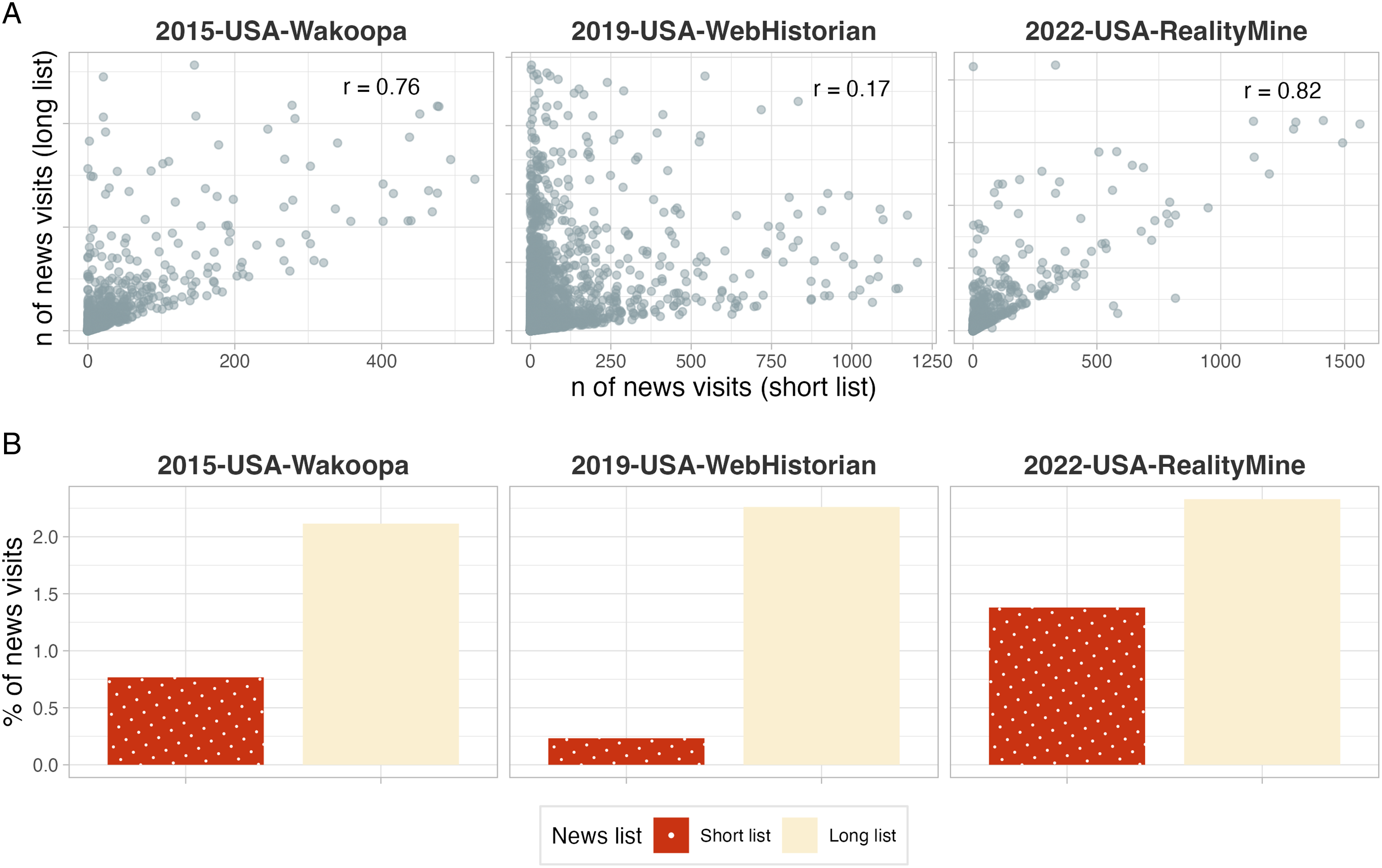

Because of the power-law distribution of most browsing behaviors (cf. Section “Accounting for Skewness”), it may be tempting to rely on a shorter list of the “most important” domains. Indeed, Bosch and Revilla (2022b, p.20) advise that beyond the fifty most visited domains, “little additional predictive power [is] gained with extra tracked [domains].” However, it is difficult to know ex ante what the top domains are, and longer lists are an insurance against missing relevant visits. Another important ingredient is induction: As the list developed for 2022-USA-RealityMine extracted news sites from the most frequently visited domains, its estimates of news exposure are similar to those based on the long list. We should also point out that the list length may matter less in contexts outside the US, with its highly fragmented (online) news market.

Recommendation #7: When using domain lists to classify browsing behavior, strive for complete lists and/or identify the most prevalent domains in your data.

Another observation regarding list compilation concerns the risk of over-coverage, as a domain may represent more than the target behavior. For example, both of the lists analyzed above classify all visits to “nytimes.com” as news consumption. This ignores the possibility that some people only visit the New York Times to play Wordle. Similarly, some visits to multi-purpose platforms such as “yahoo.com” may represent news consumption but most do not. Researchers can make use of paths or subdomains such as “yahoo.com/news” to make their list as targeted as possible (cf. Bosch & Revilla, 2022a)—or, if no fine-grained URLs are available, should consider dropping such sites from the list (cf. Gentzkow & Shapiro, 2011).

Recommendation #8: When identifying browsing behaviors via domains, avoid over-coverage by making use of paths and subdomains.

Automated Classification

As an alternative to lists, researchers can use automated API-based tools such as Webshrinker or Klazify. Most of these are commercial, although some open-source packages exist (e.g., Chintalapati & Sood, 2022). In contrast to academic list compilations, the methodology of commercial tools tends to be opaque. They also tend to lack granularity: For example, Webshrinker relies on the existing Interactive Advertising Bureau’s web content taxonomy with very general categories such as “Technology & Computing” or “Arts & Entertainment.”

For other purposes, automated classification has the potential to capture content at the right level. For example, projects studying news consumption could use the Webshrinker category “News/Weather/Information.” To compare an automated with a list-based classification, we fed domains from the 2019-USA-WebHistorian data into the Webshrinker API. Table 5 shows that most domains categorized as news via our curated list are also classified as such by Webshrinker, although only 72.37% with high confidence. However, almost 50% of domains not on our news list are classified as news.

Table 5.

Webshrinker Domain Classification Versus List-Based Classification of Domains From the 2019-USA-WebHistorian Data set (Excluding Those With Fewer Than Five Visits).

		Webshrinker
		News (high conf.)	News (low conf.)	Non-news	Not classified	Total
Domain list	News	901 (72.37%)	276 (22.17%)	68 (5.46%)	0 (0%)	1245 (100%)
Domain list	Non-news	1698 (1.7%)	45929 (45.88%)	50994 (50.94%)	1491 (1.49%)	100112 (100%)

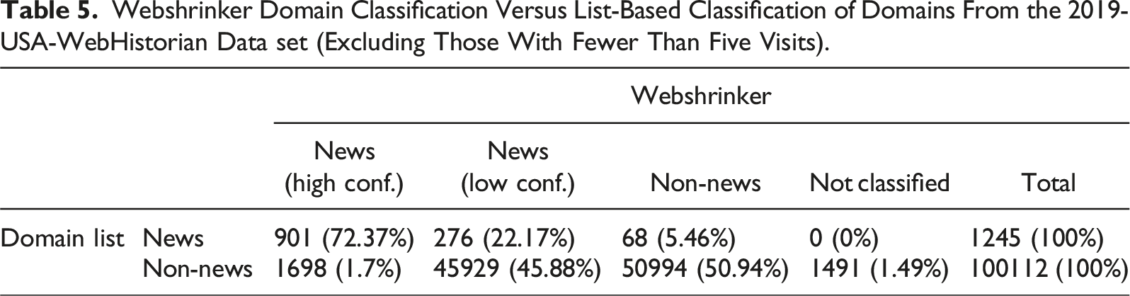
A cursory look at these cases suggests that only few are real news pages, and most of them are indeed false positives, even including misinformation sites. We thus advise researchers be aware of the uncertainty attached to automatic classification. The developments in large language models such as ChatGPT open up exciting avenues for domain classification but are still awaiting extensive validation by the scholarly community.

Recommendation #9: Manually validate automated classification tools to get a sense of accuracy.

Classifying by Website Content

Browsing data allow researchers to analyze the content seen by participants, which can be collected with scraping and parsing techniques and classified with natural-language processing (NLP). As browsing data collection typically only provides URLs, content scraping commonly happens ex post. This is fraught with several difficulties. As these issues apply beyond browsing data, we only briefly review them here. First, retrieving URL content gets more difficult as time passes. Many URLs are dynamic and change their content by design. For instance, it is impossible to reconstruct the content seen on home pages ex post. Additionally, some content becomes inaccessible over time. Showcasing this point, a recent study by Dahlke et al. (2023) found that accessibility of news and misinformation content decreased over time. Still, the rate of decay was modest, with over ninety percent of content still accessible after a year. Importantly, however, the distribution of accessible content was biased across sub-groups.

Recommendation #10: When scraping URL content ex post, be aware of dynamic and decaying web content; report the decay rate of web content; and check whether decay has distributional consequences that may affect results.

Second, the unique website architecture of every domain makes parsing meaningful text while discarding irrelevant HTML boilerplate a challenge. It is impossible to create specific parsers for (hundreds of) thousands of domains to extract the relevant information. Hence, to get scraped content into shape, researchers can exploit the power-law distribution of website visits. For some research contexts such as news, custom-made packages like newspaper3k in Python (Ou-Yang, 2013) enable easy parsing of the most popular news sites.

Recommendation #11: When scraping and parsing URL content, reuse solutions targeting your specific research context and consider ignoring the long tail of the domain distribution.

When parsing of textual data has worked sufficiently well, a lot of different text-as-data approaches can be applied (Grimmer et al., 2022). Successful applications in political communication include the distinction between political and non-political content based on binary classifiers (Guess, 2021; Stier et al., 2022) or the use of BERT-based models to identify content related to misinformation (Hoes et al., 2022). Automated text analysis is rapidly evolving, with large language models the latest point in case, and future studies may even identify more complex concepts in web content, for example, moral language.

Classifying by Website Titles or Paths

Another useful data point to classify a web visit is its HTML title, which is a technical term for the text shown on a browser tab (see Figure 6) and sometimes, but not always, is equivalent to whatever the page is “titled” with. It is particularly useful when the URL points to a non-public web page such as email services or document editors. In this case, the title can give a clue as to what kind of information a user saw. Donated-data tools such as WebHistorian provide titles by default. Titles are not typically included in tracked data but can be collected ex post. An important property of titles is that they are easier to scrape than the complete content of a web page, as SM B.4.2 illustrates.

Figure 6.

Title of the Google search for “trace data” is “trace data - Google Search.”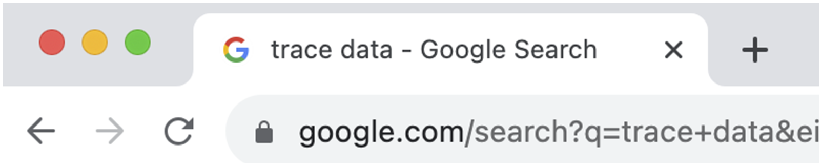

However, some of the difficulties with scraping entire pages, such as decaying URLs, URLs changing their titles, and researcher location affecting scraping results, also affect titles. To illustrate the patchiness of ex-post scraping, we took a random set of 1,000 unique URLs from one of our data sets and scraped the titles (four years after original collection). For 22.5% of URLs, the title could no longer be retrieved; for 61%, the new title did not exactly match the original title; and only 16.6% were exactly the same.

When scraped successfully, titles enable NLP classification that may rival classification of whole pages. A study by Wojcieszak, Menchen-Trevino, et al. (2023) fine-tuned a BERT-based neural classifier of titles to detect whether pages were political or non-political, achieving an F1 score of 91% for data from three languages. Despite the potential of titles and the relative ease of collecting them, few other studies have exploited them for classification.

Finally, we point researchers to the paths of URLs, which often contain human-readable text similar to titles. As described in Section “Extracting paths and queries”, paths can be directly extracted from the URL and therefore are not vulnerable to problems like web site decay. As mentioned, the path of “https://www.theguardian.com/politics/2023/aug/01/boris-johnson-swimming-pool-newts-oxfordshire” contains a clear clue about the content. Anecdotal evidence points to the potential of classifiers based on paths only.¹

Recommendation #12: As an alternative to scraping entire web pages, consider using URL titles or paths to classify web visits.

Modelling Browsing Data

As with any type of data, modelling browsing data are dictated by the chosen focus and the research goal, for example, cross-sectional designs versus more complex hierarchical models. However, browsing data exhibit some particularities that open up a veritable jungle of forking paths.

Visit-Based versus Time-Based Exposure

Individual-level browsing can be measured as a count of visits—or as the duration of exposure. Practically speaking, the strength or intensity of engagement with content can be operationalized with both visit- and time-based approaches. In a visit-based paradigm, researchers can disregard visits shorter than a certain cutoff (e.g., 3 seconds, Mangold et al., 2022). In a purely time-based approach, a continuous duration variable can be created by the (summed) visit lengths.

For most research questions, the duration of engagement with content should matter theoretically and is increasingly targeted by researchers (e.g., Hosseinmardi et al., 2021; Mangold et al., 2022). The choice between visits and time should first and foremost be motivated by theoretical considerations. Time-based measures may be more conceptually interpretable, whereas the unit of “one visit” can mean different things on different web sites. What is more, time-based measures arguably lend themselves more naturally to comparisons with other media types such as television (Allen et al., 2020; Muise et al., 2022) and make desktop versus mobile app use more comparable.

If the research question does not yield a clear preference, researchers can use both approaches to probe the robustness of their results. As we show in SM A.4, the two measures are commonly highly correlated and often yield similar conclusions (e.g., Guess, 2021; Shen & Sood, 2023; Wojcieszak, de Leeuw, et al., 2023). However, such consistency is not guaranteed. To explore the sensitivity of results to the choice between time and visits, we run cross-sectional regressions of political knowledge (survey-measured)² on exposure to news, once measured in terms of duration, once measured in terms of visits, controlling for individual background characteristics.

For each data set, Figure 7 plots the two exposure coefficients next to each other. While the directions generally are the same, in some cases we obtain a statistically significant association in one case but not the other. The plot highlights another important insight: Although magnitudes seemingly differ between the two measures, this is a complete artefact of scaling, as time-based and visit-based coefficients are not easily comparable—another reason why the choice should be theoretically motivated. If, for example, a one-visit increase is associated with a greater change in the outcome than a one-second increase, that does not make the visit-based association “bigger.”

Figure 7.

Time- versus visits-based exposure. For each dataset, we run two models, each time regressing political knowledge (rescaled to 0–100) on news exposure, age, gender, education, ideology, and overall browsing. In one model, news exposure is measured in aggregated minutes; in the other, as a count of visits. Coefficients are shown with 95%-CI. y-Axes differ across facets to account for different scales of the independent variable and varying sample sizes. Only data sets with a survey measure of political knowledge were included.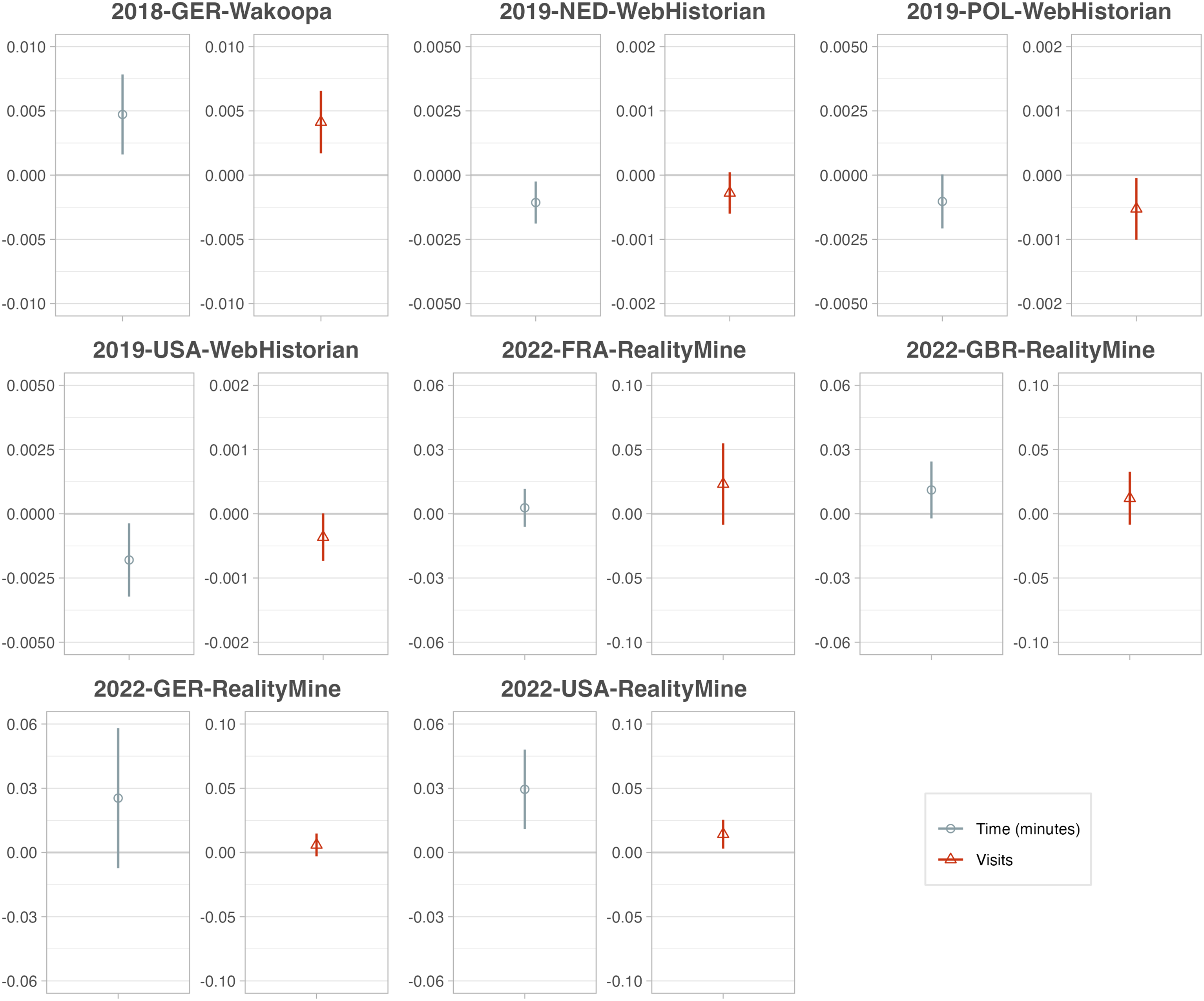

Recommendation #13: Decide whether your research question requires visits- or time-based exposure measurements, and test whether your findings are robust to both approaches.

Accounting for Skewness

Raw quantities of browsing behaviors—whether in terms of visits or time spent—are most often extremely right-skewed with a large number of zeroes. Whatever the type of browsing, a few people are likely to do it a lot and most people little or none at all. We illustrate this in SM A.5 by plotting the distributions of exposure to social media and news. For example, across the data sets, a good portion of people never visit Facebook—between 10.1% and 23.8%—while a few use it a lot.

When browsing behaviors are used as dependent variables, assumptions of linear regression models are usually violated. General advice for modelling non-negative, right-skewed outcomes applies. Browsing behavior measured in visits can be modelled with (zero-inflated) Poisson regression or negative binomial regression (as used by Möller et al., 2020; Stier, Kirkizh, et al., 2020; Stier et al., 2022). Browsing behavior measured as a duration can be interpreted as a non-negative continuous distribution. We refer readers to the statistical literature regarding such outcomes (Min & Agresti, 2002).

Regarding skewed independent variables, it is common across the social sciences to apply logarithmic transformations, and also practiced by many browsing-data studies including some of our own (e.g., Guess, 2021; Möller et al., 2020; Scharkow et al., 2020; Wojcieszak, de Leeuw, et al., 2023)—mostly without much justification. Figure 8 shows how log-transformation can impact findings. Again regressing political knowledge on time-based news exposure—once in minutes and once in hours—and controls, we either log-transform the exposure variable or not. Statistically significant coefficients sometimes become insignificant after log-transformation, and the effect of log-transformation also depends on the scale of a time-based variable. Since neither minutes nor hours are the “right” unit for duration, this opens up many degrees of freedom.

Figure 8.

Impact of log-transformation. For each dataset, we run four models, each regressing political knowledge (rescaled to 0–100) on news exposure, age, gender, education, ideology, and overall browsing. News exposure is either measured in minutes or hours and is either log-transformed (by adding one and taking the natural logarithm) or not. Coefficients are shown with 95%-CI. y-Axes differ across facets to account for different scales of the independent variable and varying sample sizes. Only data sets with a survey measure of political knowledge were included.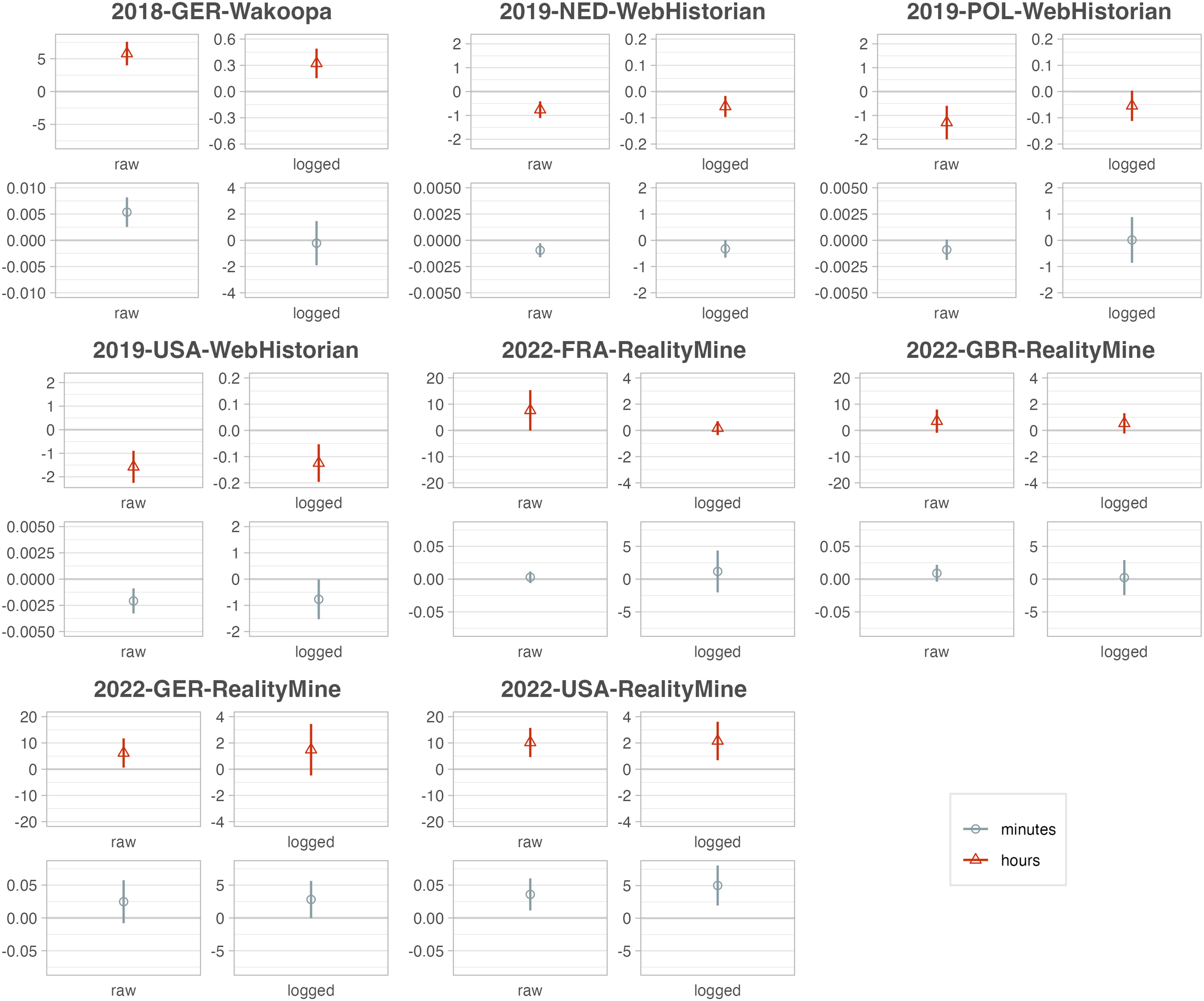

As log-transformation risks making modelling decisions less transparent—and yields less interpretable coefficients—is it advisable? Researchers should keep in mind that normally distributed independent variables are not an assumption for linear regression. Log-transformation may be motivated, first, to account for non-linear effects, and second, to reduce the impact of outliers. A recent simulation study from epidemiology—which deals with similarly skewed “exposures”—shows that outlier influence should be less of a concern than non-linear data-generating processes (Choi et al., 2022). In other words, do we have reasons to assume that a one-unit increase in the independent variable affects the outcome to the different degrees at different scale points?

Recommendation #14: Consider whether log-transforming browsing behavior is warranted by the assumed data-generating process.

Controlling for Overall Browsing

Just as specific browsing behaviors are power-law distributed, so is the general amount of browsing. As those who do more of some specific browsing are also likely to do more browsing in general, any measure of a specific behavior risks being confounded. In SM A.6, we illustrate how exemplary browsing behaviors are strongly correlated with overall browsing. To take such correlations into account for descriptive estimates, researchers can normalize the variable in question, for example, by using the proportion out of overall browsing or taking an average number of visits per time unit, for example, per day.

When a specific browsing behavior is used as an independent variable in a model, confounding can be avoided by adding overall browsing as a control variable, or by using normalizations such as the proportion out of all browsing. To illustrate the sensitivity to such choices, we again run our toy regression of political knowledge on number of news visits plus covariates, either not controlling or controlling for overall browsing, or using a proportional news exposure variable. As Figure 9 shows, in some cases, a significant effect of news exposure disappears once overall browsing is controlled for.

Figure 9.

Impact of controlling for overall browsing. For each dataset, we run three models, each regressing political knowledge (rescaled to 0–100) on news exposure, age, gender, education, ideology, and visits to news sites. We either do not control, control for overall browsing (in visits), or use the proportion of visits to news sites out of all visits. Coefficients of news exposure are shown with 95%-CI. y-Axes differ across facets to account for different scales of the independent variable and varying sample sizes. Only data sets with a survey measure of political knowledge were included.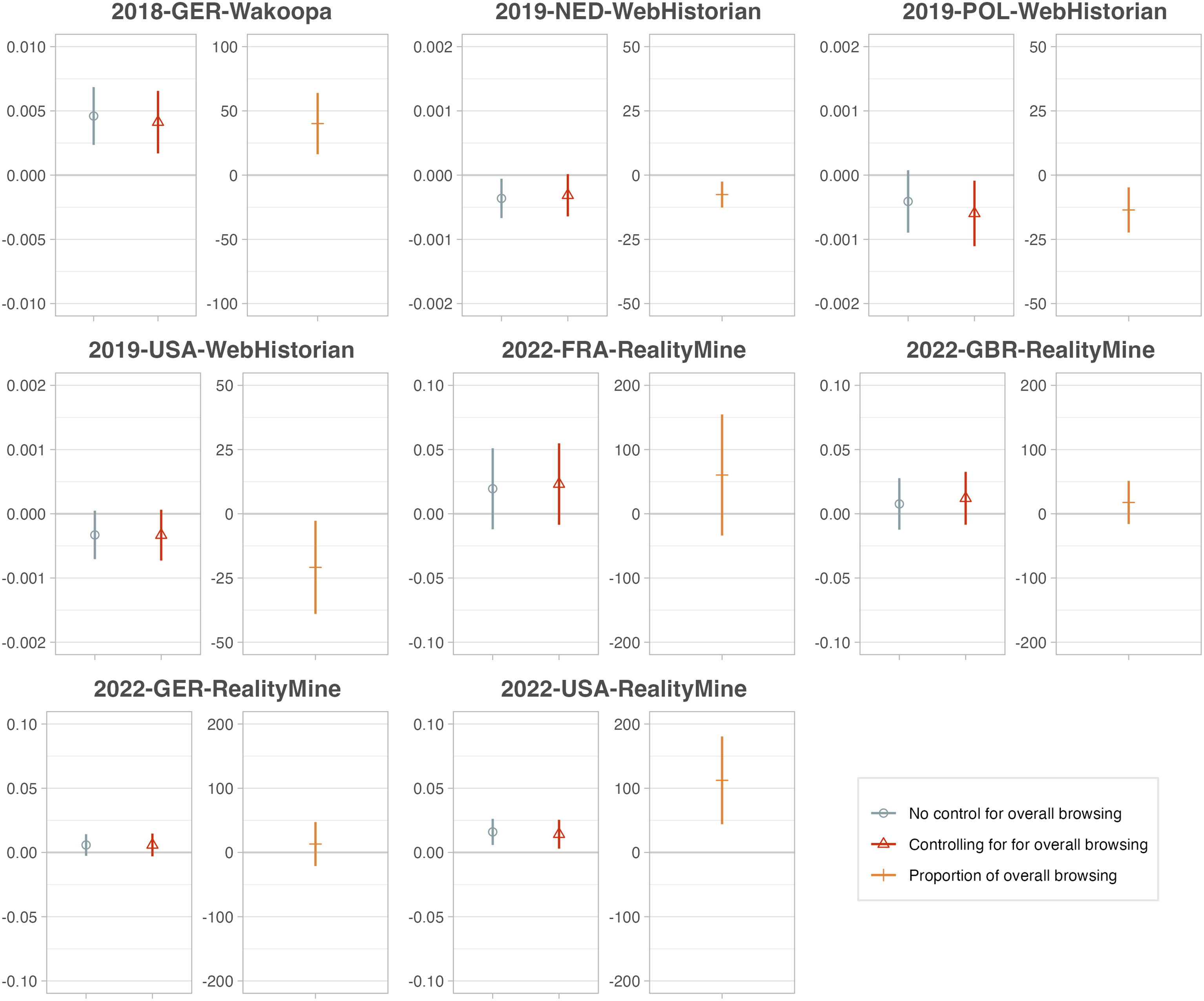

However, such adjustments must be theoretically motivated. In a model that controls for overall browsing, the coefficient for a specific browsing behavior estimates the difference in the outcome for subjects with the same overall browsing frequency. This may not always be the desired estimand. Consider an experiment that encourages subjects to engage more in a specific browsing behavior. The increase in this behavior would be identical to the increase of overall browsing, and controlling for overall browsing would bias the treatment effect downwards. A similar problem could arise for models targeting within-person changes in a browsing behavior.

Recommendation #15: Consider whether your research question requires adjusting for overall browsing frequency.

Causal Inference

The entire literature on media effects revolves around the idea that exposure to certain information causally influences behaviors and attitudes (e.g., Valkenburg et al., 2016). At the same time, scholars have been equally interested in what causes information diets (e.g., Katz et al., 1973). Two ways to isolate causal effects are experiments and observing people over time. Each comes with its own challenges when applied to browsing data.

Experimental Designs

Randomly “encouraging” study participants to adopt certain media consumption behaviors is not new. However, the possibility of partially observing behavior over the course of the study with browsing data increases potential for precise measurement and has motivated a number of recent studies (e.g., Aslett et al., 2022; Casas et al., 2022; Guess et al., 2021; Wojcieszak et al., 2022). We point out three ways in which browsing data can be useful for experiments.

Measuring Compliance

When conducting experiments using encouragement designs, researchers need to address non-compliance. Browsing data are extremely useful for gauging whether a treatment has successfully encouraged changes in media consumption. How to analyze experimental data with a compliance measure is discussed in standard textbooks (e.g., Gerber & Green, 2012). One challenge particular to browsing data is that it is difficult to decide what constitutes sufficient compliance. For example, if subjects are encouraged to consume more of a certain news outlet (e.g., Guess et al., 2021), should one count a few more news visits as compliance? As compliance in browsing is inherently continuous, researchers will be confronted with degrees of compliance. Although it may be tempting to coarsen compliance into a binary variable, methodological research suggests that this can lead to bias (Marshall, 2016). Compliance patterns may also be complicated by pre-treatment imbalance caused by a few outliers with high levels of the behavior in question.

Recommendation #16: In experimental design encouraging certain browsing behavior, measure compliance as a continuous variable.

Measuring Outcomes

Browsing data offer the tantalizing possibility of measuring genuine changes in information consumption following random interventions. For example, researchers may want to study the effect of behavioral nudges on the share of untrustworthy websites visited by participants. Two recent studies illustrate potential design trade-offs. Aslett et al. (2022) randomly incentivized installation of a browser extension designed to provide news quality labels in users’ search and social feeds, detecting significant effect heterogeneity by pre-treatment information diet. Testing a different intervention in the context of a survey experiment, Guess, Lerner, et al. (2020) collected web tracking data to measure effects of a digital media literacy intervention on subjects’ browsing behavior, finding no measurable effect on consumption of fake news, mainstream news, or fact-checking sites.

Both studies construct dependent variables using browsing data, but they differ in their mode of treatment delivery: in the “field” (via the browser extension) versus within a survey. The resulting gap in treatment strength is likely a major explanation for the divergence in the pattern of results. Specifically, treatment effects in surveys are often short-lived to begin with, and thus it will be difficult to detect any small shifts in browsing behavior—which may also be swamped by natural patterns of within-person variability. This is a disappointing reality, as part of the initial promise of digital behavioral data was the ability to observe effects beyond the survey or lab environment.

Despite this bias-variance tradeoff, browsing data can still be informative as outcome measures when treatments are delivered outside the survey environment and with sufficient strength. For example, the study by Guess et al. (2021) was powered to detect standardized effects of moderate size (Cohen’s d ≈ 0.10) on certain types of visits. The minimum detectable effect for browsing-based outcomes in this study is similar to those found in Aslett et al. (2022). This could be a good starting point for researchers gauging statistical power.

Recommendation #17: When measuring browsing behavior as an outcome, gauge plausible effect sizes in order to estimate statistical power.

Pre-Treatment Covariates

Browsing data can also be useful in experiments for constructing pre-treatment covariates designed to improve precision. The aforementioned noise inherent to trace-based variables can be dampened through judicious selection of pre-treatment measures. An additional benefit of collecting pre-treatment browsing data is that it can be used to verify design assumptions, for example, by checking balance across treatment conditions.

Recommendation #18: Collect pre-treatment browsing data for use as prognostic covariates and to help verify design assumptions.

Panel Designs

For many research questions involving browsing data, randomization may not be possible. Panel design offers an alternative path to causal inference: By measuring both the independent variable—say, online gaming—and the dependent variable—say, mental well-being—for an individual at multiple time points, one can test whether they both move along with each other. Under what circumstances causal inference is plausible with such panel data is discussed elsewhere (e.g., Vaisey & Miles, 2017). We just point out two important issues particularly relevant for web browsing panel data.

Time-Varying Confounders

Even with the most conservative techniques such as fixed-effects models, unobserved confounders that vary over time and across subjects will bias causal estimates. For example, if subjects over the course of the study started spending more time with friends, this may affect both mental well-being and online gaming, which will bias estimates if not controlled for. The example illustrates that realistically, there are many variables beyond web browsing that may confound the relationship under study. Researchers should strive to measure such potential confounders in surveys.

Recommendation #19: When using browsing behavior as an independent variable in panel modelling, measure as many time-varying confounders as possible.

Within-Unit Variation

The second point pertains to the tradeoff between within- and between-subject variation. Some modelling techniques, such as fixed-effects models, rely exclusively on within-subject variation. Others, such as random-effects models or “within-between models” (Allison, 2009), exploit both. In theory, fixed-effects models are an attractive choice for researchers using web tracking data for causal inference. The issue is that browsing behaviors often vary little within individuals over time.

To illustrate, we explore the within- and between-subject variation of visits to various social media platforms and news in our multiple-wave data sets. Table 6 shows the standard deviation of each exposure in the first wave (between-subjects variation), as well as the average standard deviation within each user (within-subjects variation). Across data sets and browsing behaviors, the latter is much lower than the former. In SM A.7.1, we present these variations in terms of visit duration.

Table 6.

Comparing Within- and Between-Person Variation of Social Media and News Consumption. “Within” Reports the Average Within-Person (i.e., Across Waves) Standard Deviation of the Number Visits. “Between” Reports the Between-Person Standard Deviation of the Number of Visits of One wave. Only Multi-Wave Data Sets Included.

	Facebook		Reddit		Twitter		YouTube		News
	Within	Between	Within	Between	Within	Between	Within	Between	Within	Between
2018-GER-Wakoopa	806.7	1709.2	6.4	72.0	58.9	339.2	566.1	1180.8	281.0	627.8
2019-NED-WebHistorian	296.9	1939.2	11.6	320.8	24.9	520.2	89.4	575.1	170.7	1216.2
2019-POL-WebHistorian	663.9	2590.3	2.7	252.7	17.7	558.8	250.7	974.7	405.5	1251.8
2019-USA-WebHistorian	630.2	2594.2	250.8	1187.6	137.4	1147.7	260.0	1112.5	502.5	1977.4
2022-ESP-Wakoopa	178.4	71.7	25.3	18.4	100.2	43.7	193.2	30.5	91.0	22.8
2022-FRA-RealityMine	405.1	332.3	12.9	2.2	51.0	98.0	223.1	272.6	59.6	87.2
2022-GBR-RealityMine	233.1	229.7	2.4	7.9	79.0	153.8	60.0	133.8	113.5	122.8
2022-GER-RealityMine	318.3	326.7	1.5	6.9	32.2	881.2	138.2	1076.3	133.3	283.8
2022-USA-RealityMine	384.0	523.2	14.3	85.4	147.1	735.9	130.1	287.1	134.4	269.3

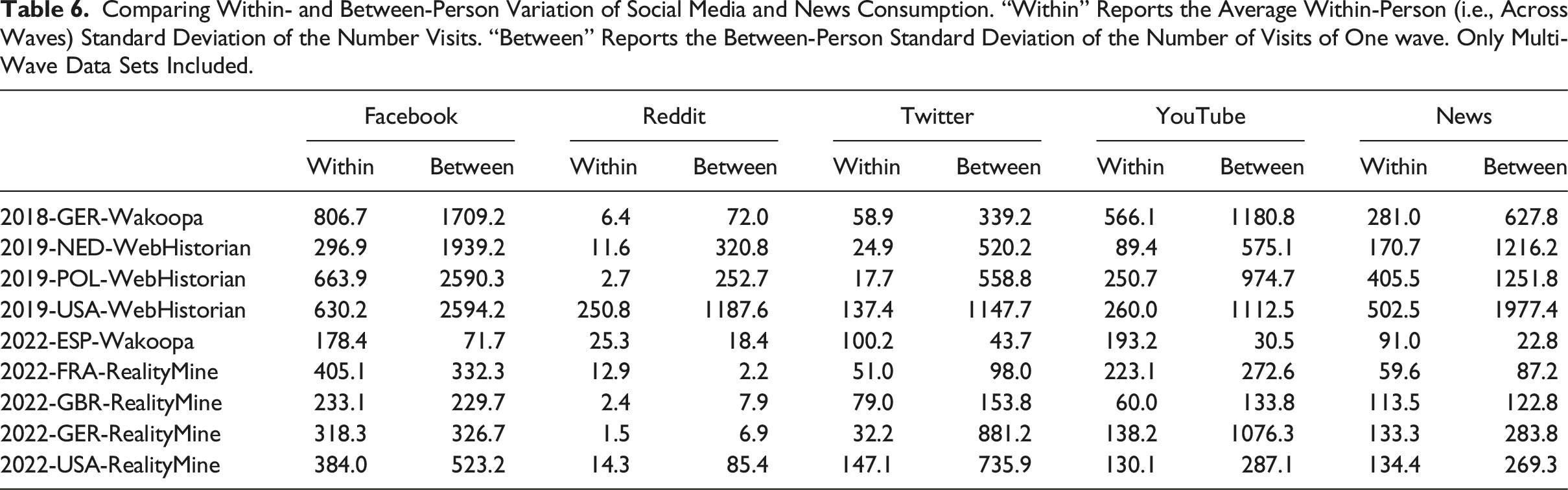
Researchers need to take this fact into account when making modelling choices, ideally through some ex-ante power simulations. Informed by the empirical results shown above, we ran such simulations (SM A.7.2), specifically varying the amount of within-unit variation. Fixed-effects models quickly become statistically underpowered with a realistic amount of within-unit variation.

Recommendation #20: When using browsing behavior as an independent variable in panel modelling, estimate statistical power given plausible within-subject variation.

Discussion

Web browsing data are an increasingly important resource for researchers studying digital behavior. Whichever way they are collected, researchers typically have to preprocess browsing data, decide whether to drop certain observations, classify visits, and finally engage in statistical modelling. Along each of these steps, we have illustrated and given guidance on the many necessary decisions.

Our recommendations have highlighted some general characteristics of web browsing data. First, the data collection itself is contingent on the chosen tool, and researchers should try to understand how pre-measured variables in their browsing data were generated (cf. Section “Pre-processing Browsing Data”). When relying on commercial tools, we often do not know exactly how variables were created. We hope that in the future, the scientific community will break open the black box of commercial technologies—or better still, create their own solutions. Transparency about the intricacies of data collection will make preprocessing decisions much more straightforward and enhance reproducibility.

Second, the explorations of our own data sets illustrate that researchers have to make difficult decisions about how and whether to exclude any data (cf. Section “Filtering Browsing Data”) and be mindful of and transparent about any potential implications these decisions have on their estimates. We have also pointed to the potential of browsing data that has not been tapped by previous studies. For example, making use of website titles or human-readable parts of URLs may be a comparably effortless yet accurate way to categorize web visits (cf. Section “Classifying Browsing Data”). Recent advances in and the continued development of large language models open up additional avenues to classify online contents.

Finally, when it comes to modelling, we pointed out how browsing data diverge from other types of data social scientists are familiar with. These particularities require well-informed modelling decisions (cf. Section “Modelling Browsing Data”). The discussion of modelling issues has also highlighted that browsing data offer many opportunities—for example, incorporating a fine-grained temporal dimension—but also have limits: for many behaviors of interest, there is little signal; behaviors may change relatively little within individuals over time; and habits may be difficult to change with experimental interventions.

We do not claim to have presented complete solutions for every analytical decision, especially since our own research and data are necessarily limited to certain topics. However, we tried to review studies from across disciplines and hope that the recommendations we formulate here will start a discussion about best practices in the (computational) social sciences. We think such a debate is necessary, since many existing studies—including our own—have not consistently justified all of their analytical decisions.

Supplemental Material

Supplemental Material - Analysis of Web Browsing Data: A Guide

Supplemental Material for Analysis of Web Browsing Data: A Guide by Bernhard Clemm von Hohenberg, Sebastian Stier, Ana S. Cardenal, Andrew M. Guess, Ericka Menchen-Trevino, and Magdalena Wojcieszak in Social Science Computer Review.

Footnotes

Declaration of Conflicting Interests

The author(s) declared no potential conflicts of interest with respect to the research, authorship, and/or publication of this article.

Funding

The author(s) disclosed receipt of the following financial support for the research, authorship, and/or publication of this article: The authors gratefully acknowledge the support of the European Research Council, “Europeans exposed to dissimilar views in the media: investigating backfire effects”, Proposal EXPO-756301 (ERC Starting Grant, PI Magdalena Wojcieszak). Any opininos, findings and conclusions or recommendations expressed in this material are those of the authors and do not necessarily reflect the views of the funders.

ORCID iDs

Bernhard Clemm von Hohenberg

Sebastian Stier

Supplemental Material

Supplemental material for this article is available online.

Notes

Author Biographies

Bernhard Clemm von Hohenberg is a Research Associate at the GESIS – Leibniz Institute for the Social Sciences in Cologne. His research in computational social science revolves around misinformation and media effects, using experimental methods, surveys and trace data.

Sebastian Stier is a Scientific Director of the Computational Social Science department at GESIS – Leibniz Institute for the Social Sciences in Cologne and Professor at the School of Social Sciences, University of Mannheim. He investigates the quality and scientific value of digital behavioral data and uses such data for substantive research on the impact of digital media on societies and democracy.

Ana S. Cardenal is a Professor of Political Science at the Universitat Oberta de Catalunya (UOC) and a Lecturer at the Universitat Pompeu Fabra (UPF). Her current research interests focus on digital and social media, online news audiences, preferences and opinion formation, and the use of computational methods in the social sciences.

Andrew M. Guess is Assistant Professor of Politics and Public Affairs, and affiliated faculty at the Center for Information Technology Policy at Princeton University. His research on digital media and politics has investigated the extent to which online news diets are polarized, patterns in the consumption and spread of online misinformation, and the effects of feed ranking algorithms on social platforms.

Ericka Menchen-Trevino earned her PhD in the Meida Technology and society program of the School of Communication at Northwestern University. She previously worked as an Assistant Professor at Erasmus University in Rotterdam and at American University. Her research interests lie at the intersection of political communication and digital media studies, with a focus on methodology.

Magdalena Wojcieszak (PhD Annenberg School of Communication, University of Pennsylvania) is a Professor of Communication at UC Davis. She examines exposure to (political) information online and the effects of this exposure on extremity, polarization, and (mis)perceptions.

References

Adam

Makhortykh

Maier

Aigenseer

Urman

Gil-Lopez

Christner

de León

Ulloa

(2023). Improving the quality of individual-level online information tracking: Challenges of existing approaches and introduction of a new content- and long-tail sensitive academic solution. Unpublished working paper.

Allen

Howland

Mobius

Rothschild

Watts

D. J.

(2020). Evaluating the fake news problem at the scale of the information ecosystem. Science Advances, 6(14), Article eaay3539. https://doi.org/10.1126/sciadv.aay3539

Allison

P. D.

(2009). Fixed effects regression models, Sage publications.

Aslett

Guess

A. M.

Bonneau

Nagler

Tucker

J. A.

(2022). News credibility labels have limited average effects on news diet quality and fail to reduce misperceptions. Science Advances, 8(18), Article eabl3844. https://doi.org/10.1126/sciadv.abl3844

Bachl

Link

Mangold

Stier

(2023). Search engine use for health-related purposes: Behavioral data on online health information-seeking in Germany, OSF.

Barseghyan

(2013). Tld. https://pypi.org/project/tld

Bosch

O. J.

Revilla

(2022a). The challenges of using digital trace data to measure online behaviors: Lessons from a study combining surveys and metered data to investigate affective polarization, Sage Research Methods.

Bosch

O. J.

Revilla

(2022b). When survey science met web tracking: Presenting an error framework for metered data. Journal of the Royal Statistical Society: Series A, 185(Suppl 2), S408–S436. https://doi.org/10.1111/rssa.12956

Cahan

Bai

(2023). Factor-based imputation of missing values and covariances in panel data of large dimensions. Journal of Econometrics, 233(1), 113–131. https://doi.org/10.1016/j.jeconom.2022.01.006

10.

Cardenal

A. S.

Galais

Majó-Vázquez

(2019). Is facebook eroding the public agenda? Evidence from survey and web-tracking data. International Journal of Public Opinion Research, 31(4), 589–608. https://doi.org/10.1093/ijpor/edy025

11.

Casas

Menchen-Trevino

Wojcieszak

(2022). Exposure to extremely partisan news from the other political side shows scarce boomerang effects. Political Behavior, 45(4), 1491–1530. https://doi.org/10.1007/s11109-021-09769-9

12.

Chintalapati

Sood

(2022). Piedomains: Predict the kind of content hosted by a domain based on domain name and content, Harvard.

13.

Choi

Buckley

J. P.

Kuiper

J. R.

Keil

A. P.

(2022). Log-transformation of independent variables: Must we? Epidemiology, 33(6), 843–853. https://doi.org/10.1097/EDE.0000000000001534

14.

Christner

Urman

Adam

Maier

(2022). Automated tracking approaches for studying online media use: A critical review and recommendations. Communication Methods and Measures, 16(2), 79–95. https://doi.org/10.1080/19312458.2021.1907841

15.

Clemm von Hohenberg

Ventura

Wojcieszak

Nagler

Tucker

(2024). Survey professionalism: New evidence from browsing data. https://osf.io/vr7gb/

16.

Cronin

Gon¸ calves

J. F. F.

Wojcieszak

Clemm von Hohenberg

Menchen-Trevino

(2022). The (null) over-time effects of exposure to local news websites:Evidence from trace data. Journal of Information Technology and Politics, 20(4), 1–15.

17.

Dahlke

Kumar

Durumeric

Hancock

(2023). Pie metrics: Quantifying the systematic bias in the ephemerality and inaccessibility of web scraping content from url-logged web-browsing digital trace data, OSF.

18.

Fitzmaurice

Davidian

Verbeke

Molenberghs

(2008). Longitudinal data analysis, CRC Press.

19.

Fletcher

Kalogeropoulos

Nielsen

R. K.

(2021). More diverse, more politically varied: How social media, search engines and aggregators shape news repertoires in the united kingdom. New Media and Society, 25(8). https://doi.org/10.1177/14614448211027393

20.

Gentzkow

Shapiro

J. M.

(2011). Ideological segregation online and offline. Quarterly Journal of Economics, 126(4), 1799–1839. https://doi.org/10.1093/qje/qjr044

21.

Gerber

A. S.

Green

D. P.

(2012). Field experiments: Design, analysis, and interpretation, W. W. Norton.

22.

Grimmer

Roberts

M. E.

Stewart

B. M.

(2022). Text as data: A new framework for machine learning and the social sciences, Princeton University Press.

23.

Guess

A. M.

(2021). Almost) everything in moderation: New evidence on Americans’ online media diets. American Journal of Political Science, 65(4), 1007–1022. https://doi.org/10.1111/ajps.12589

24.

Guess

A. M.

Barberá

Munzert

Yang

(2021). The consequences of online partisan media. Proceedings of the National Academy of Sciences of the United States of America, 118(14), Article e2013464118. https://doi.org/10.1073/pnas.2013464118

25.

Guess

A. M.

Lerner

Lyons

Montgomery

J. M.

Nyhan

Reifler

Sircar

(2020). A digital media literacy intervention increases discernment between mainstream and false news in the United States and India. Proceedings of the National Academy of Sciences of the United States of America, 117(27), 15536–15545. https://doi.org/10.1073/pnas.1920498117

26.

Guess

A. M.

Nyhan

Reifler

(2020). Exposure to untrustworthy websites in the 2016 us election. Nature Human Behaviour, 4(5), 472–480. https://doi.org/10.1038/s41562-020-0833-x

27.

Hoes

Clemm von Hohenberg

Gessler

Wojcieszak

Qian

(2022). The cure worse than the disease? How the media’s attention to misinformation decreases trust, OSF. https://doi.org/10.31234/osf.io/4m92p

28.

Hosseinmardi

Ghasemian

Clauset

Mobius

Rothschild

D. M.

Watts

D. J.

(2021). Examining the consumption of radical content on youtube. Proceedings of the National Academy of Sciences of the United States of America, 118(32), Article e2101967118. https://doi.org/10.1073/pnas.2101967118

29.

Howison

Wiggins

Crowston

(2011). Validity issues in the use of social network analysis with digital trace data. Journal of the Association for Information Systems, 12(12), 767–797. https://doi.org/10.17705/1jais.00282

30.

Kalogeropoulos

Fletcher

Nielsen

R. K.

(2019). News brand attribution in distributed environments: Do people know where they get their news? New Media and Society, 21(3), 583–601. https://doi.org/10.1177/1461444818801313

31.

Katz

Blumler

J. G.

Gurevitch

(1973). Uses and gratifications research. Public Opinion Quarterly, 37(4), 509–523. https://doi.org/10.1086/268109

32.

Keusch

Kreuter

(2021). Digital trace data: Modes of data collection, applications, and errors at a glance. Handbook of computational social science, Taylor and Francis.

33.

Keyes

Jacobs

Schmidt

(2019). Urltools: Vectorised tools for URL handling and parsing. https://cran.r-project.org/package=urltools

34.

Little

R. J.

Rubin

D. B.

(2019). Statistical analysis with missing data, John Wiley and Sons.

35.

Mangold

Stier

Breuer

Scharkow

(2022). The overstated generational gap in online news use? A consolidated infrastructural perspective. New Media and Society, 24(10), 2207–2226. https://doi.org/10.1177/1461444821989972

36.

Marshall

(2016). Coarsening bias: How coarse treatment measurement upwardly biases instrumental variable estimates. Political Analysis, 24(2), 157–171. https://doi.org/10.1093/pan/mpw007

37.

Menchen-Trevino

(2016). Web historian: Enabling multi-method and independent research with real-world web browsing history data, Illinois Ideals.

38.

Menchen-Trevino

Karr

C. J.

(2022). Understanding individual web browsing: Social media use in context (126), The Sage Handbook of Social Media Research Methods.

39.

Menchen-Trevino

Struett

Weeks

B. E.

Wojcieszak

(2023). Searching for politics: Using real-world web search behavior and surveys to see political information searching in context. The Information Society, 39(2), 98–111. https://doi.org/10.1080/01972243.2022.2152915

40.

Min

Agresti

(2002). Modeling nonnegative data with clumping at zero: A survey, University of Florida.

41.

Möller

van de Velde

R. N.

Merten

Puschmann

(2020). Explaining online news engagement based on browsing behavior: Creatures of habit? Social Science Computer Review, 38(5), 616–632. https://doi.org/10.1177/0894439319828012

42.

Mozilla Foundation . (2022). Public suffix list, Mozilla Foundation. https://publicsuffix.org/

43.

Muise

Hosseinmardi

Howland

Mobius

Rothschild

Watts

D. J.

(2022). Quantifying partisan news diets in web and tv audiences. Science Advances, 8(28), Article eabn0083. https://doi.org/10.1126/sciadv.abn0083

44.

Nelson

J. L.

Webster

J. G.

(2017). The myth of partisan selective exposure: A portrait of the online political news audience. Social Media + Society, 3(3), 205630511772931. https://doi.org/10.1177/2056305117729314

45.

Ou-Yang

(2013). Newspaper3k: Article scraping and curation, Newspaper3k. https://newspaper.readthedocs.io/en/latest

46.

Santos

B. D. L.

Hortaçsu

Wildenbeest

M. R.

(2012). Testing models of consumer search using data on web browsing and purchasing behavior. The American Economic Review, 102(6), 2955–2980. https://doi.org/10.1257/aer.102.6.2955

47.

Scharkow

Mangold

Stier

Breuer

(2020). How social network sites and other online intermediaries increase exposure to news. Proceedings of the National Academy of Sciences of the United States of America, 117(6), 2761–2763. https://doi.org/10.1073/pnas.1918279117

48.

Schmidt

Mangold

Stier

Ulloa

(2023). Facebook as an avenue to news: A comparison and validation of approaches to identify facebook referrals, OSF. https://osf.io/preprints/socarxiv/cks68.

49.

Schoch

Chan

C.-H.

(2023). adaR: A fast ’WHATWG’ compliant URL parser. https://CRAN.R-project.org/package=adaR

50.

Schoch

Clemm Von Hohenberg

Stier

Mangold

(2023). webtrackR: Analysing web tracking data and online news behaviour. https://CRAN.R-project.org/package=webtrackR

51.

Shen

Sood

(2023). Holier than thou: Partisan gap in the consumption of pornography online, Gaurav Sood.

52.

Silber

Breuer

Beuthner

Gummer

Keusch

Siegers

Stier

Weiss

(2022). Linking surveys and digital trace data: Insights from two studies on determinants of data sharing behavior. Journal of the Royal Statistical Society Series A: Statistics in Society, 185(Suppl_2), S387–S407. https://doi.org/10.1111/rssa.12954

53.

Stier

Breuer

Siegers

Thorson

(2020). Integrating survey data and digital trace data: Key issues in developing an emerging field. Social Science Computer Review, 38(5), 503–516. https://doi.org/10.1177/0894439319843669

54.

Stier

Kirkizh

Froio

Schroeder

(2020). Populist attitudes and selective exposure to online news: A cross-country analysis combining web tracking and surveys. The International Journal of Press/Politics, 25(3), 426–446. https://doi.org/10.1177/1940161220907018

55.

Stier

Mangold

Scharkow

Breuer

(2022). Post post-broadcast democracy? News exposure in the age of online intermediaries. American Political Science Review, 116(2), 768–774. https://doi.org/10.1017/s0003055421001222

56.

Toth

Trifonova

(2021). Somebody’s watching me: Smartphone use tracking and reactivity. Computers in Human Behavior Reports, 4, 100142. https://doi.org/10.1016/j.chbr.2021.100142

57.

Ulloa

Kacperski

C. S.

(2023). Search engine effects on news consumption: Ranking and representativeness outweigh familiarity in news selection, Sage.

58.

Vaisey

Miles

(2017). What you can—and can’t—do with three-wave panel data. Sociological Methods and Research, 46(1), 44–67. https://doi.org/10.1177/0049124114547769

59.

Valkenburg

P. M.

Peter

Walther

J. B.

(2016). Media effects: Theory and research. Annual Review of Psychology, 67, 315–338. https://doi.org/10.1146/annurev-psych-122414-033608

60.

Van Buuren

(2018). Flexible imputation of missing data, CRC Press.

61.

von Andrian-Werburg

M. T.

Siegers

Breuer

(2023). A re-evaluation of online pornography use in Germany: A combination of web tracking and survey data analysis. Archives of Sexual Behavior, 52(8), 3491–3503. https://doi.org/10.1007/s10508-023-02666-8

62.

Wojcieszak

Clemm von Hohenberg

Casas

Menchen-Trevino

de Leeuw

Gonçalves

Boon

(2022). Null effects of news exposure: A test of the (un) desirable effects of a ‘news vacation’and ‘news binging. Humanities and Social Sciences Communications, 9(1), 413–510. https://doi.org/10.1057/s41599-022-01423-x

63.

Wojcieszak

de Leeuw

Menchen-Trevino

Lee

Huang-Isherwood

K. M.

Weeks

(2023). No polarization from partisan news: Over-time evidence from trace data. The International Journal of Press/Politics, 28(3), 601–626. https://doi.org/10.1177/19401612211047194

64.

Wojcieszak

Menchen-Trevino

Clemm von Hohenberg

de Leeuw

Gon¸ calves

Davidson

Gon calves

(2023). Non-news websites expose people to more political content than news websites: Evidence from browsing data in three countries. Political Communication, 41(1), 129–151. https://doi.org/10.1080/10584609.2023.2238641

65.

Wojcieszak

Menchen-Trevino

Goncalves

J. F. F.

Weeks

(2021). Avenues to news and diverse news exposure online: Comparing direct navigation, social media, news aggregators, search queries, and article hyperlinks, The International Journal of Press/Politics.

Supplementary Material

Please find the following supplemental material available below.

For Open Access articles published under a Creative Commons License, all supplemental material carries the same license as the article it is associated with.

For non-Open Access articles published, all supplemental material carries a non-exclusive license, and permission requests for re-use of supplemental material or any part of supplemental material shall be sent directly to the copyright owner as specified in the copyright notice associated with the article.

0.00 MB

11.23 MB