Sage Journals: Discover world-class research

Abstract

Social and behavioral studies more and more often yield multi-block data, which consist of novel blocks of data (e.g., data from wearable devices) and traditional blocks of data (e.g., survey data) collected from the same sample. Multi-block data offer researchers valuable insights into complex social mechanisms, where several influences act together. Yet such mechanisms are likely to differ among subgroups. Hence, fully revealing the composite mechanisms underlying multi-block data is challenging, since proper clustering analysis of such data requires methods that simultaneously detect the covariation of variables underlying all data blocks and the group differences therein. Additionally, the methods should be able to handle high-dimensional datasets, which might include many irrelevant variables. Here, we present Clusterwise Sparse Simultaneous Component Analysis (CSSCA), a method that groups the subjects that are driven by the same mechanisms and, at the same time, extracts cluster-specific components that model these mechanisms. By imposing structure constraints, CSSCA further distinguishes common mechanisms that underlie all data blocks from distinctive mechanisms that only underlie one or a few data blocks. In extensive simulations, CSSCA delivered convincing results in recovering the clusters and their associated component structures across various conditions. More importantly, CSSCA showed a clear advantage over existing methods when substantial cluster differences in the component structure were present. We demonstrated the usefulness of CSSCA in an application to data stemming from a study on personality.

Keywords

clustering data integration high-dimensional data analysis

Introduction

Thanks to recent technological developments and the increasing adaption of data-rich research in social and behavioral sciences (Gil de Zuniga & Diehl, 2017), novel types of data such as genetic data, global positioning system coordinates, and social media data are collected more and more often, along with traditional sociodemographic and questionnaire data (Hofferth et al., 2017). Such linked data that contain different types of measurements, collected from the same sample, are labeled multi-block data. In the domain of communication science, for example, Wells and Thorson (2017) proposed and demonstrated a novel method to examine political content flows by linking social media data with survey data. Another example comes from Vargo and Hopp (2017), who identified the connections between individuals’ political polarization and their extent of civil conversation with a multi-block of tweets and census data.

Research based on multi-block data has the potential to advance social and behavioral sciences: It offers opportunities to obtain novel insights into complex social mechanisms where several influencing factors—each of them reflected by a particular data block—act jointly. Let us consider an illustrative example of multi-block data, as depicted in Figure 1A, with rows referring to subjects and columns representing variables. The multi-block data consist of two blocks: one block of self-reported motivations (each column represents one type of motivation) and one block of degree of physical activities, measured by wearable devices and aggregated across several time intervals (each column represents the average degree of physical activity per hour). With such multi-block data, health psychologists would be able to investigate how various motivations of participants are related to their patterns of physical activities.

Figure 1.

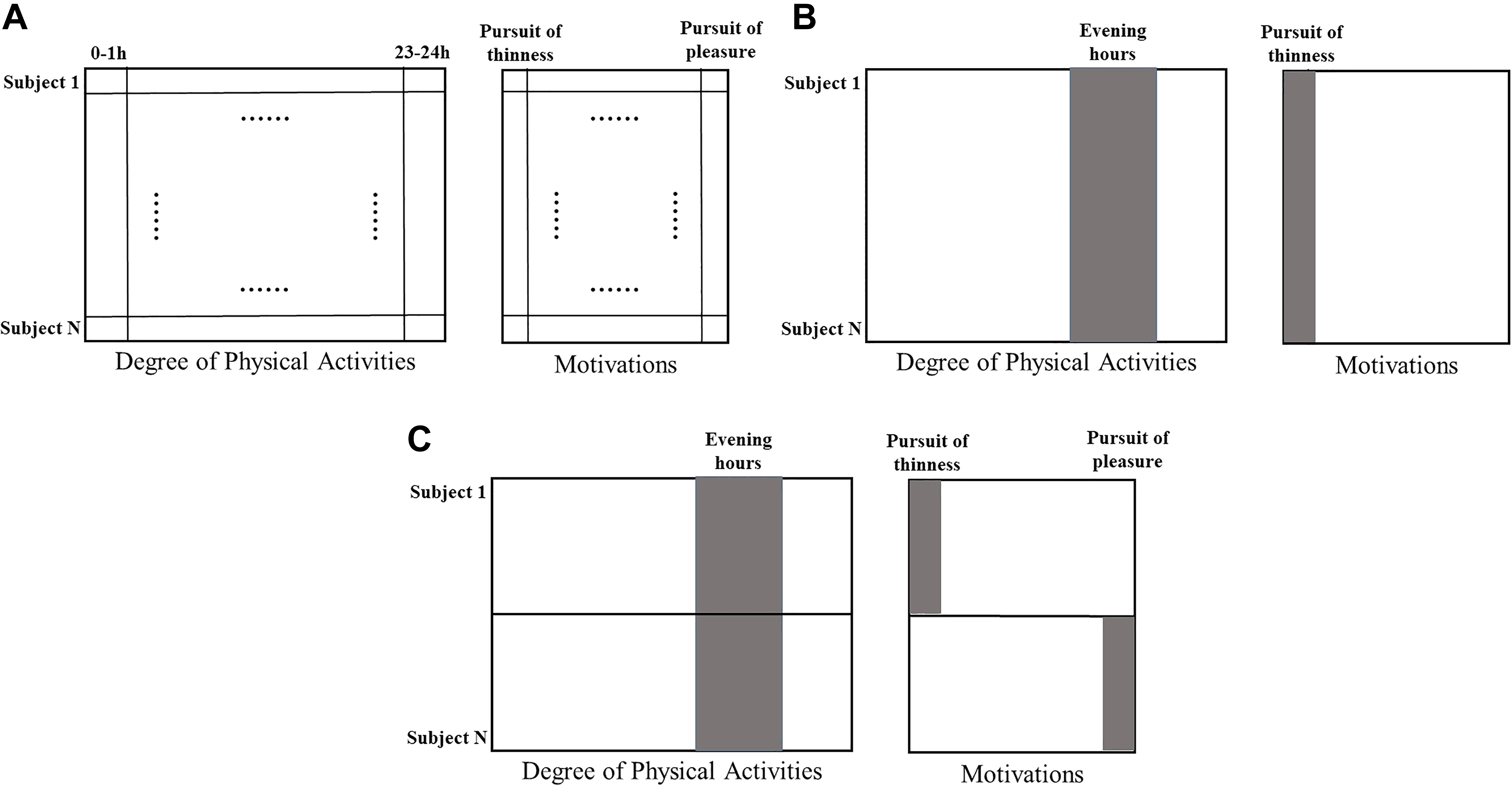
Graphic visualization of the illustrative example. The multi-block data include two data blocks, with column entries referring to variables and row entries to subjects. (A) The data structure of multi-block data; (B) A potential outcome of a data analysis that reveals variables that are associated between the different data blocks (marked with gray color); and (C) Heterogeneity between subjects in the variables that are associated between the data blocks.

Because of a lack of theoretical knowledge about the novel types of data and (or) its linkage with traditional data, exploratory analyses could offer important insights in the structure of the data (Fan, Han, & Liu, 2014). In our illustrative example, appropriate exploratory analyses should detect crucial yet subtle links between motivations on the one hand, reflected by some variables in the self-report data block, and patterns of physical activity on the other hand, reflected by several variables in the physical activity data block. A potential outcome is illustrated in Figure 1B, with the columns marked by gray implying associations between variables from different data blocks: Figure 1B demonstrates that the pursuit of thinness is linked with intensive physical activities during evening hours. In essence, the aim of multi-block data analysis is to identify the common variation—typically implying synergistic actions between variables—which underlies all data blocks and to pick up its associated linked variables (De Roover, Timmerman, Mesquita, & Ceulemans, 2013; Van Deun, Wilderjans, Van den Berg, Antoniadis, & Van Mechelen, 2011).

A unique feature of the multi-block data is that in addition to the common variation, they contain distinctive variation, which refers to the covariation between variables from one or a few, but not all, data blocks (Lock, Hoadley, Marron, & Nobel, 2013; Van Deun et al., 2011). Concerning our illustrative example, while the researchers mainly want to detect the common variation (i.e., the covariation of motivations and certain patterns of physical activities), the multi-block data may also include distinctive variation such as response styles in the self-report of motivations (e.g., Harzing, 2006) and individual baseline levels of physical activity in the data derived from wearable devices. Hence, to extract the common variation that is typically of interest, it is necessary to separate out the distinctive variation, which, in some cases, might also contain substantive information that is of interest to the researchers.

Because of the presence of both common and distinctive variation in the multi-block data, conventional ways of analyzing such multi-block data might be less desirable. On the one hand, principal component analysis (PCA; Jolliffe, 2011; Meredith & Millsap, 1985) could be performed on the concatenated data blocks to summarize the association between variables by a few components. However, such an analysis would only detect the components explaining the largest (co)variation across the blocks, which are likely to be a mixture of common and distinctive variation. Therefore, this approach is not able to uncover both common and distinctive variation. On the other hand, one could also first perform a separate analysis (e.g., PCA) on each data block and then integrate the results over all data blocks. However, as pointed out by Wang and Gu (2016), this approach of data analysis has two noteworthy shortcomings: (1) It is likely to omit the important common variation, and (2) its performance deteriorates with increasing disparities between the results of separate analyses.

Recently, some component-based integrative analysis methods, most noticeably joint and individual variation explained (Lock et al., 2013) and DISCO-SCA (Schouteden, Van Deun, Pattyn, & Van Mechelen, 2013), have been introduced and gained substantial popularity in multi-block data analysis. A particularly useful feature of these methods is the capability to effectively distinguish the common and distinctive variation. These methods have been successfully applied in psychology (e.g., Chawarska, Ye, Shic, & Chen, 2016; Gu & Van Deun, 2019), neuroscience (e.g., Yu, Risk, Zhang, & Marron, 2017), and medicine (Sandri et al., 2018), among other research fields. Nevertheless, these methods fail to overcome two additional challenges of multi-block data analysis.

First, multi-block data frequently include novel types of data of a high-dimensional nature (i.e., an equal or greater number of variables than subjects). With very little theoretical guidance, researchers often, by default, include all information they have gathered in the analysis, leading to the involvement of a substantial amount of redundant information (Waldherr, Maier, Miltner, & Günther, 2017). This severely hampers the interpretation of the components and makes it intricate to reveal the variables that are most interesting for further investigation since the components may correlate with a large number of irrelevant variables (Zou, Hastie, & Tibshirani, 2006). Therefore, methods are needed that can automatically and effectively filter out the irrelevant variables. Note that the common practice of neglecting variables with small loadings (i.e., treating them as zero loadings) yields a suboptimal solution, as first discussed in Cadima and Jolliffe (1995).

Another challenge of analyzing multi-block data is the heterogeneity among subjects: Subgroups may be present in the data that differ in the patterns of covariation (Jung & Wickrama, 2008). In our illustrative example, the association between motivations and degree of physical activities may differ among subjects. For instance, as demonstrated in Figure 1C, degree of physical activity in the evening hours may be found associated with the pursuit of thinness among some subjects (the first half) and with the pursuit of pleasure among the others (the second half). Such subgroups are often not known to the researchers beforehand. Hence, a clustering method is needed that can reveal the subgroups of subjects such that only the subjects of the same subgroup have the same pattern of covariation.

To respond to these challenges, we present Clusterwise Sparse Simultaneous Component Analysis (CSSCA), a novel method designed for multi-block data analysis. CSSCA assigns all subjects to mutually exclusive clusters, such that the subjects that belong to the same cluster hold the same common and distinct components, while the subjects that belong to different clusters are assumed to vary on different common and distinctive components.

The remainder of the article is organized into five sections: in the Methods section, we will formally introduce CSSCA and contrast it with several existing methods. In the Algorithm and Model Selection section, the algorithm, as well as a model selection procedure for CSSCA, is introduced. The performance of CSSCA and its model selection procedure are evaluated in the Simulation Studies section. The usefulness of CSSCA for applied psychological research is demonstrated in the Application section. Finally, the implications, limitations, and a blueprint for future research are elaborated in the Discussion section.

To increase the accessibility of the method, we have made CSSCA, its model selection procedure, as well as other auxiliary functions, available in the R package “ClusterSSCA.” The package can be downloaded freely from https://github.com/syuanuvt/CSSCA. On the same web page, we have also provided a step-by-step user guide to facilitate the usage of CSSCA in applied research.

Method

In this section, we present CSSCA by specifying the assumed data generating model and objective function used. First, however, we introduce multi-block data from the formal point of view and discuss existing methods that serve as the building blocks of CSSCA.

Multi-Block Data

Multi-block data consist of multiple blocks of data containing information about the same group of respondents (Tenenhaus & Tenenhaus, 2014). More formally, each of the L data blocks X _l (N × J_l) (l = 1, 2,…, L) contains values of N subjects on J_l variables. A popular framework for analyzing multi-block data is simultaneous component analysis (SCA; Kiers & ten Berge, 1989; Van Deun, Smilde, van der Werf, Kiers, & Van Mechelen, 2009), from which CSSCA originates.

SCA

Similar to PCA, SCA reduces the dimensions of all data blocks simultaneously and results in a few components that maximally account for the total variation across the data blocks. Formally, the SCA model is represented by Equation 1 (see Timmerman & Kiers, 2003).

X_{l} = T P_{l}^{T} + E_{l}

where T with size N × R denotes the simultaneous component scores on R components (i.e., T is assumed to be the same for each of the data blocks), P _l with size J_l × R denotes the component loadings of the variables in the l^th data block, and E _l with size N × J_l denotes the error matrix associated with the l^th data matrix X _l . For SCA-based methods, usually all variables are mean-centered and standardized (see Van Deun et al., 2009). To identify the solution, Equation 1 is made subject to suitable constraints, for example, a principal axis orientation in combination with orthogonality of the component scores: T ^T T = I.

The objective of SCA is to minimize the sum of squares of residuals, given by

min_{T, P^{con}} {‖ X^{con} - T P^{{con}^{T}} ‖}_{2}^{2}

subject to T ^T T = I, where X ^con of size N × J denotes the concatenated data matrix (J equals the total number of variables across all data blocks) and ${‖ X^{con} - T P^{{con}^{T}} ‖}_{2}^{2}$ denotes the square of the Frobenius norm of $(X^{con} - T P^{{con}^{T}})$ . P ^con with size J × R is then the concatenated component loading matrix.

As pointed out in Van Deun, Wilderjans, Van den Berg, Antoniadis, and Van Mechelen (2011), SCA fails to appropriately address two of the important challenges of multi-block data analysis. First, interpretation of the resulting components is daunting as it is based on contributions of all variables. Second, the components obtained by SCA do not account for the block structure, in particular, they do not separate the common and distinctive sources of variation. Solutions have been proposed to address the two drawbacks of SCA, resulting in SSCA (i.e., sparse SCA) with common and distinctive components.

SSCA With Common and Distinctive Components

To tackle the first challenge of automatic variable selection and thus to ease the interpretation of components, especially in dealing with high-dimensional datasets, regularization (e.g., l₀ norm regularization, or lasso regularization) has been used to shrink some component loadings to (exactly) zero (hereafter, these entries will be called sparseness-induced zero loadings), leading to SSCA (Van Deun et al., 2011). Different forms of regularization can be used in SSCA; here, in developing CSSCA, we adopt the l₀ norm regularization (also known as a cardinality constraint). This norm fixes the number of zero elements in the loading matrices to a predefined number with a range between 0 and J × R and thus allows to fix the proportion of zero elements (called the level of sparsity hereafter and indicated by spar()).

To approach the second challenge of discerning common and distinctive constructs, Schouteden et al. (2013) have proposed DISCO-SCA that determines the status of components (i.e., common or distinctive components) through rotations. To further avoid the post hoc rotations, Gu and Van Deun (2019) directly imposed zero loadings in a structured way, which results in an unambiguous status of each component. Specifically, to define a distinctive component, except for the variables of the block(s) that the component is supposed to underlie, all other loadings on this distinctive component are fixed to zero (the zero loadings are hereafter called the distinctiveness-induced zero loadings). We illustrate this for a loading matrix that includes both sparseness-induced zero loadings and distinctiveness-induced zero loadings in Figure 2. The depicted loading matrix includes seven variables (rows) from two data blocks (the first data block has four variables while the second has three) and four components (columns), and zero loadings are denoted by “0” while nonzero loadings are denoted by “×.” In the figure, the first two components are sparse common components, since they are associated with variables from both data blocks. The third component, with all nonzero loadings for variables in Block 1, is a sparse distinctive component that pertains to Block 1. In the same vein, the fourth component can be regarded as a sparse distinctive component that pertains to Block 2.

Figure 2.

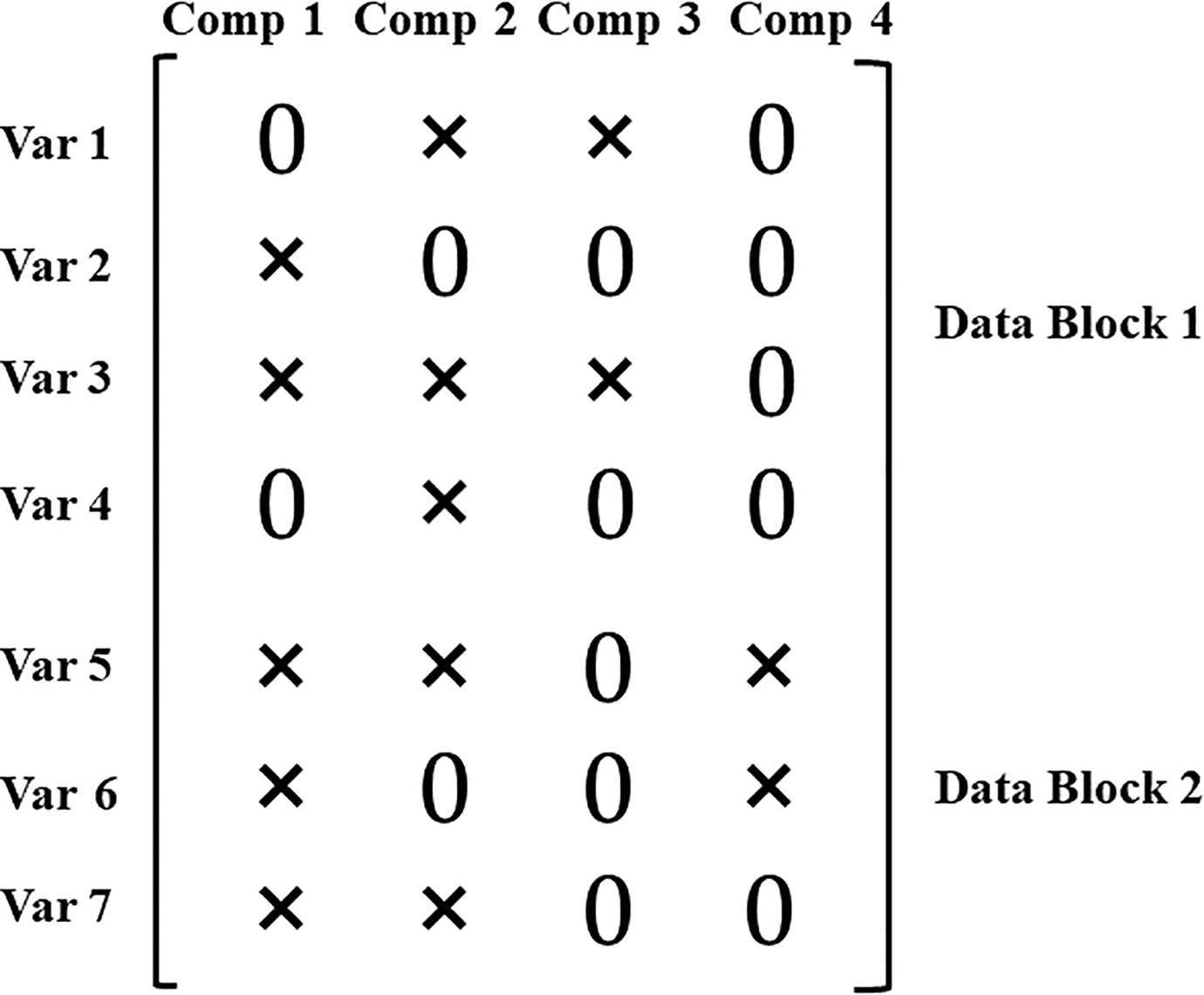
An example of common and distinctive components in a concatenated loading matrix. The components are represented in columns, while the variables are indicated by rows. The first two components are defined as common components, while the third and fourth components are distinctive components pertaining to Block 1 and Block 2, respectively. Var j = j^th variable and Comp r = r^th component.

Formally, for the analysis of SSCA with common and distinctive components, the objective function is described in

min_{T, P^{con}} {‖ X^{con} - T P^{{con}^{T}} ‖}_{2}^{2}

subject to (i) T ^T T = I, (ii) spar(P ^con) = S, where S is a predefined number between 0 and 1 that indicates a predefined level of sparsity of the loading matrices, and (iii) distinctiveness-induced zero loadings are prespecified in P ^con to impose common and distinctive components.

CSSCA

CSSCA extends SSCA to account for heterogeneity in the mean structure and the component structure. Specifically, instead of assuming that the same component loading matrix pertains to all subjects, a few loading matrices are assumed to underlie the multi-block data where each applies to a particular subgroup of subjects. CSSCA aims to detect these subgroups (also called clusters) and their associated mean structure and component structure.

Model and Objective Function

Formally, the cluster-specific model of CSSCA on the level of the concatenated data is given by

X_{k}^{con} = μ_{k}^{con} + Τ_{k} P_{k}^{{con}^{T}} + E_{k} (k = 1, \dots, k)

subject to (i) ${T_{k}}^{T} T_{k} = I$ , (ii) $spar (P_{k}^{con}) = S$ , and (iii) distinctiveness-induced zero loadings are prespecified in $P_{k}^{con}$ to force common and distinctive components. In Equation 4, $X_{k}^{con} (N_{k} \times J)$ , T _k (N_k × R), and $P_{k}^{con} (J \times R)$ denote the concatenated data, the component score matrix, and the component loading matrix of cluster k, respectively, while $μ_{k}^{con} (N_{k} \times J)$ with all identical rows represents the mean structure of the k^th cluster. Note that, in addition to these constraints, CSSCA assumes the same number of common components and also the same structure of distinctive components for each of the clusters. In other words, the method assumes that the dimensions of the loading matrices as well as the positions of distinctiveness-induced zero loadings are identical across clusters. This is because we would like to keep CSSCA a simple method in terms of model selection and interpretation.

The objective function of CSSCA is presented in Equation 5, where we minimize the total sum of squares of the residuals.

min_{μ_{k}, T_{k}, P_{k}^{con}} {\sum_{k = 1}^{K} ‖ X_{k}^{con} - μ_{k}^{con} - T_{k} P_{k}^{{con}^{T}} ‖}_{2}^{2}

subject to (i) ${T_{k}}^{T} T_{k} = I$ , (ii) $spar (P_{k}^{con}) = S$ , and (iii) prespecified distinctiveness-induced zero loadings in $P_{k}^{con}$ .

Related Methods

A number of related dimension reduction based clustering methods have been developed for the analysis of single-block data: for example, reduced K-means (Stute & Zhu, 1995), factorial K-means (Vichi & Kiers, 2001), and subspace K-means (Timmerman, Ceulemans, De Roover, & Van Leeuwen, 2013). As argued in Introduction, the clustering analyses on the concatenated dataset fail to distinguish the common and distinctive components. Thus, they are less desirable in the analysis of multi-block data.

Recently, some clustering methods for multi-block data have been proposed in the field of bioinformatics. In their systematic review, Wang and Gu (2016) classified all these methods into two categories, and they demonstrated the advantages of the methods with a direct integrative clustering strategy, which, instead of first performing a separate clustering analysis on each data block and then integrating all partitions, accounts for all data blocks simultaneously. CSSCA, with its simultaneous dimension reduction of all data blocks, clearly falls into this category.

Among the clustering methods that also employ the direct integrative approach, iCluster (Shen, Olshen, & Ladanyi, 2009) is a popular choice, and it also lays the basis for several succeeding methods, including the low-rank approximation clustering method (LRAcluster; Wu, Wang, Zhang, & Gu, 2015) and joint and individual clustering (Hellton & Thoresen, 2016). In essence, iCluster projects the high-dimensional data onto a lower dimensional subspace by summarizing the common variation over multiple data blocks into several latent variables. Subsequently, iCluster utilizes K-means clustering to obtain cluster assignments from the resulting latent variables. iCluster (and other mean-level based methods) differs from CSSCA in that iCluster assumes that all clusters possess the same covariance structure, while CSSCA does not impose such a restriction and allows the covariance structure to differ between clusters. In this respect, CSSCA offers an important extension to the existing methods.

We can briefly conclude that CSSCA is the only clustering method available so far, that, in the context of multi-block data analysis, partitions subjects based on both mean structure and covariance structure.

Algorithm and Model Selection

Algorithm

Starting from a random partition of the subjects, the CSSCA algorithm obtains an SSCA solution for each of the initial clusters. Subsequently, the procedure iterates over a loop in which the subjects are reassigned one by one: For each subject, the SSCA solution is obtained for each of the K − 1 potential reassignments, and the subject is assigned to the cluster with which the total loss is minimized (implying that the total loss is guaranteed to be nonincreasing for each update of the cluster membership). After a complete iteration of reassigning all subjects, the algorithm starts the next iteration if and only if (1) the total decrease in loss value of the current iteration is larger than a predefined value and (2) the number of iterations is smaller than a predefined maxima. Since the algorithm may result in local optima, a multistart procedure is used (e.g., De Roover et al., 2013; Timmerman et al., 2013). Using pseudocode, we present in Algorithm 1, the algorithm of CSSCA (see Section 1 of the online supplementary material). Embedded in Algorithm 1 is the iterative procedure to estimate the cluster-specific SSCA solution, which applies an alternating strategy first proposed in Gu and Van Deun (2019). In essence, Algorithm 2 iteratively optimizes $P_{k}^{con}$ conditional on T _k and optimizes T _k conditional on $P_{k}^{con}$ , using well-established optimization routines. The procedure is detailed in Algorithm 2 in the supplementary material (Section 1), also in the form of pseudocode. Similar to Algorithm 1, Algorithm 2 yields a nonincreasing sequence of loss values throughout the iterations and thus guarantees to converge to a fixed point. In Section 2 of the supplementary material, we report some technical details on the generation of the starting partitions and on some additional requirements of the model parameters. Details concerning the implementation of the CSSCA algorithm can be found in the R package.

Model Selection

To run the CSSCA algorithm, the actual model parameters (e.g., the number of clusters and the level of sparsity) need to be specified. In practice, however, researchers only have limited or no knowledge on the true values of these parameters. To facilitate the application of CSSCA, we propose a model selection procedure to determine the number of clusters and the level of sparsity with the best balance between the model fit (i.e., the total loss) and the model complexity.

Wilderjans and Ceulemans (2013) showed that a sequential model selection strategy may have several advantages. Adapted to solving the model selection problem of CSSCA, the sequential strategy includes two steps: (1) pick the optimal number of clusters K and (2) determine the optimal level of sparsity S, given the selected K. To illustrate our model selection procedure, assume that K and S are selected from ascending candidate sets (K₁, K₂,…, K_U) and (S₁, S₂,…, S_V), respectively. In the first step, as illustrated in Equation 6, the conditional scree ratio sr(K_u|S_v) is computed for each possible pair of K_u (K_u = K₂,…, K_U−1) and S_v (S_v = S₁, S₂,…, S_V)

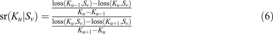
sr (K_{u} | S_{v}) = \frac{\frac{loss (K_{u - 1}, S_{v}) - loss (K_{u}, S_{v})}{K_{u} - K_{u - 1}}}{\frac{loss (K_{u}, S_{v}) - loss (K_{u + 1}, S_{v})}{K_{u + 1} - K_{u}}}

with loss (K_u, S_v) referring to the total loss resulting from the CSSCA analysis with the number of clusters set to K_u and the level of sparsity to S_v. Afterward, for each possible value of K_u (K_u = K₂,…, K_U−1), the average conditional scree ratio sr(K_u) is computed by averaging sr(K_u|S_v) over all possible values of S_v (S_v = S₁, S₂,…, S_V), as follows:

sr (K_{u}) = \frac{\sum_{v} sr (K_{u} | S_{v})}{V}

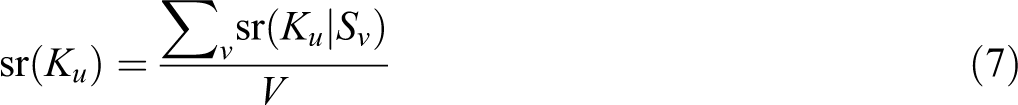
The optimal number of clusters K_opt is then determined by maximizing sr(K_u). In the second step, conditional on the optimal number of clusters K_opt, the conditional scree ratio sr(S_v|K_opt) can be calculated for each S_v (S_v = S₂,…, S_V−1), as shown in

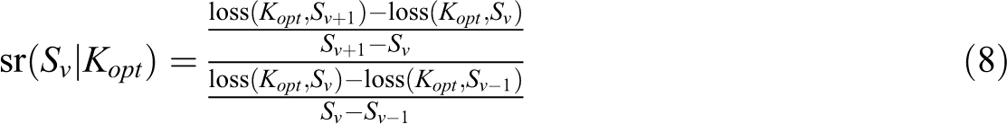
sr (S_{v} | K_{o p t}) = \frac{\frac{loss (K_{o p t}, S_{v + 1}) - loss (K_{o p t}, S_{v})}{S_{v + 1} - S_{v}}}{\frac{loss (K_{o p t}, S_{v}) - loss (K_{o p t}, S_{v - 1})}{S_{v} - S_{v - 1}}}

Again, we select the optimal level of sparsity by maximizing the conditional scree ratio.

It is important to note that, according to Equations 6 and 8, sr(K_u|S_v) is not defined if K_u = K₁ (minimum) or K_u = K_U (maximum) and sr(S_v|K_opt) is not defined when S_v = S₁ (minimum) or S_v = S_V (maximum). Therefore, the sequential approach does not allow for the selection of the minimal and maximal values of K and S.

Simulation Studies

To investigate the performance of CSSCA and its model selection procedure, we conducted two simulation studies. In Simulation Study 1, the performance of CSSCA given the correct number of clusters and level of sparsity was evaluated and compared with the performance of iCluster in various conditions. The proposed model selection procedure for CSSCA was examined in Simulation Study 2.

Simulation Study 1

Design

Three model characteristics that were expected to have relatively small impacts on the clustering performance were kept constant: the number of data blocks L = 2, the number of common components R_c = 2, and the number of distinctive components in each data block R_l = (1, 1).

The following eight factors were used to create the various conditions:

The number of variables J_l: low-dimensional condition (J_l = (15, 15)) and high-dimensional condition (J_l = (15, 50)). Hence, the total number of variables J equals 30 in low-dimensional conditions and 65 in high-dimensional conditions.

The number of clusters K: small (K = 2) and large (K = 4).

The cluster size N_k: small (N_k = 50 or 30, dependent on Factor 4), and large (N_k = 100 or 60, dependent on Factor 4).

The equality of cluster size: In the equality conditions, each cluster contains 50 or 100 subjects, while in the inequality conditions, one cluster contains 30 or 60 subjects, and the rest contain 50 or 100 subjects (see Factor 3).

The level of sparsity S (of loading matrices): low (0.3), medium (0.5), and high (0.7).

The proportion of the total variance accounted for by the noise structure, or the noise level of the data, e: low (0.1), medium (0.2), and high (0.3).

The proportion of the structural variance accounted for by the mean structure b: small (0.1), medium (0.5), and large (0.9). Since the mean structure is assumed to be equal for all subjects of the same cluster, b also represents mean-level cluster differences. Excluding the variance that is accounted for by the noise structure, the remaining (1 − e) of the total variance (which is also called structural variance hereafter) can be decomposed into variance caused by cluster differences in the mean structure and cluster differences in the component structure. In other words, b (1 − e) of the total variance can be attributed to mean-level cluster differences.

The average congruence level ϕ of cluster-specific loadings: low (approximately 0.2) and high (approximately 0.53). Here, congruence is measured by the average Tucker congruence (Haven & ten Berge, 1977; Tucker, 1951) between the cluster-specific loadings across all pairs of clusters.

In total, the full factorial design of the seven factors resulted in 2 × 2 × 2 × 2 × 3 × 3 × 3 × 2 = 864 conditions. In each condition, we generated 40 replications. Hence, a total of 34,560 datasets were created and analyzed. The data generation procedure is detailed in the supplementary material (Section 3).

Results and Discussion

Execution Time of CSSCA

Over all 34,560 datasets, the average execution time of CSSCA was 774 seconds or around 13 min. In the simulation, the maximal size of the datasets was 400 rows by 65 columns when K = 4, N_k = 100, and J = 65. For each of these datasets, CSSCA spent an average of 1,900 s or around 31 min. Overall, taking into consideration that the computation speed can be greatly improved by the parallel computation function available in the R package ClusterSSCA, the execution time of CSSCA should be acceptable for applied research.

Clustering Accuracy of CSSCA

The main indicator of the clustering performance is the clustering accuracy, that is, how well does the partition produced by CSSCA recovers the true partition (i.e., the partition used to generate the data). A widely used measure of clustering accuracy is the Adjusted Rand Index (ARI; Hubert & Arabie, 1985). ARI takes values between 0 and 1, with 0 indicating that the overlap between the two cluster partitions is at the chance level and 1 suggesting a complete overlap between the two cluster partitions. In this study, the ARI between the recovered cluster partition and the true cluster partition was used as the indicator of CSSCA’s clustering accuracy.

We expected that two of the factors—the mean-level cluster differences b and the noise level of the data e—would have the strongest impact on the clustering accuracy of CSSCA. First, a larger b means that the component structure accounts for a smaller proportion of the structural variance and, in extreme cases, can become very small compared to the error variance (e.g., the component structure accounts for 7% of the total variance while the noise accounts for 30%). In such cases, it can be expected that the component structure of some subjects is masked by the noise. Second, a larger e results in the fact that the true data structure is masked by a larger amount of noise, and the true cluster partition is therefore more difficult to be recovered.

The results of the simulations fit the expectations well. We found that both b and e were indeed among the most influential factors and that a better recovery of the clusters, averaged across replications and the other factors, was obtained when (1) b was smaller (ARI = 0.997 when b = .1, ARI = 0.999 when b = .5, and ARI = 0.986 when b = .9) and (2) e was smaller (ARI = 1 when e = .1, ARI = 0.999 when e = .2, and ARI = 0.984 when e = .3). The average clustering accuracy of CSSCA in function of the other six factors is reported in the supplementary material (Section 4).

To further investigate the effects of the interactions between b and e on the clustering accuracy of CSSCA, we examine the average ARI in cross-tabulation of the two factors, as illustrated in Table 1. In all conditions, the average ARI between the resulting partitions and true partitions was above 0.95. Thus, in general, CSSCA shows an adequate clustering performance, according to the widely adopted criterion proposed by Steinley (2004). When the proportion of mean-level differences was low or medium, CSSCA recovered the true clusters exceptionally well (i.e., ARI > 0.99), even with relatively noisy data. Table 1 also reveals that the worst ARI (0.96) is obtained for the combination of large b and large e, as expected.

Table 1.

The Means and the Standard Deviations (in Brackets) of ARI Between the True Cluster Partitions and the CSSCA-Recovered Cluster Partitions in Various Conditions.

Noise Level	Proportion of Mean-Level Differences: Low (b = .1)	Proportion of Mean-Level Differences: Medium (b = .5)	Proportion of Mean-Level Differences: High (b = .9)
Low (e = .1)	1 (0)	1 (0)	1 (0)
Medium (e = .2)	1 (0)	1 (0)	.99 (.04)
High (e = .3)	.99 (.02)	.99 (.02)	.96 (.18)

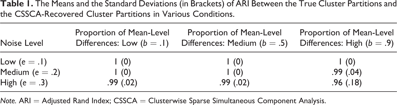
Note. ARI = Adjusted Rand Index; CSSCA = Clusterwise Sparse Simultaneous Component Analysis.

Comparison of CSSCA and iCluster in Clustering Accuracy

Figure 3 illustrates the results of the comparison between the average clustering accuracy of CSSCA and that of iCluster for various levels of b (i.e., the proportion of structural variance accounted for by the mean structure). Clearly, when the structural variance mainly pertained to the component structure (i.e., b = .1), CSSCA drastically outperformed iCluster with an ARI of 0.997 compared to only 0.105 for iCluster. In line with our expectations, CSSCA demonstrated an overwhelming advantage in clustering accuracy when the component structure is the predominant source of variation. The superior performance of CSSCA in clustering accuracy persisted when the mean structure and the component structure contributed equally to the structural variance (i.e., b = .5), where CSSCA achieved an average ARI of almost 1 (0.999 to be exact) while iCluster obtained an average ARI of 0.93. When b equaled 0.9, CSSCA could still recover the clusters very well (average ARI = 0.986), but the clusters obtained with iCluster were more accurate (average ARI = 1). In general, CSSCA has demonstrated a consistent and convincing performance in terms of clustering accuracy across all conditions. While CSSCA achieved a good clustering accuracy even in the unfavorable conditions, iCluster did not perform better than clustering by chance in the most difficult condition.

Figure 3.

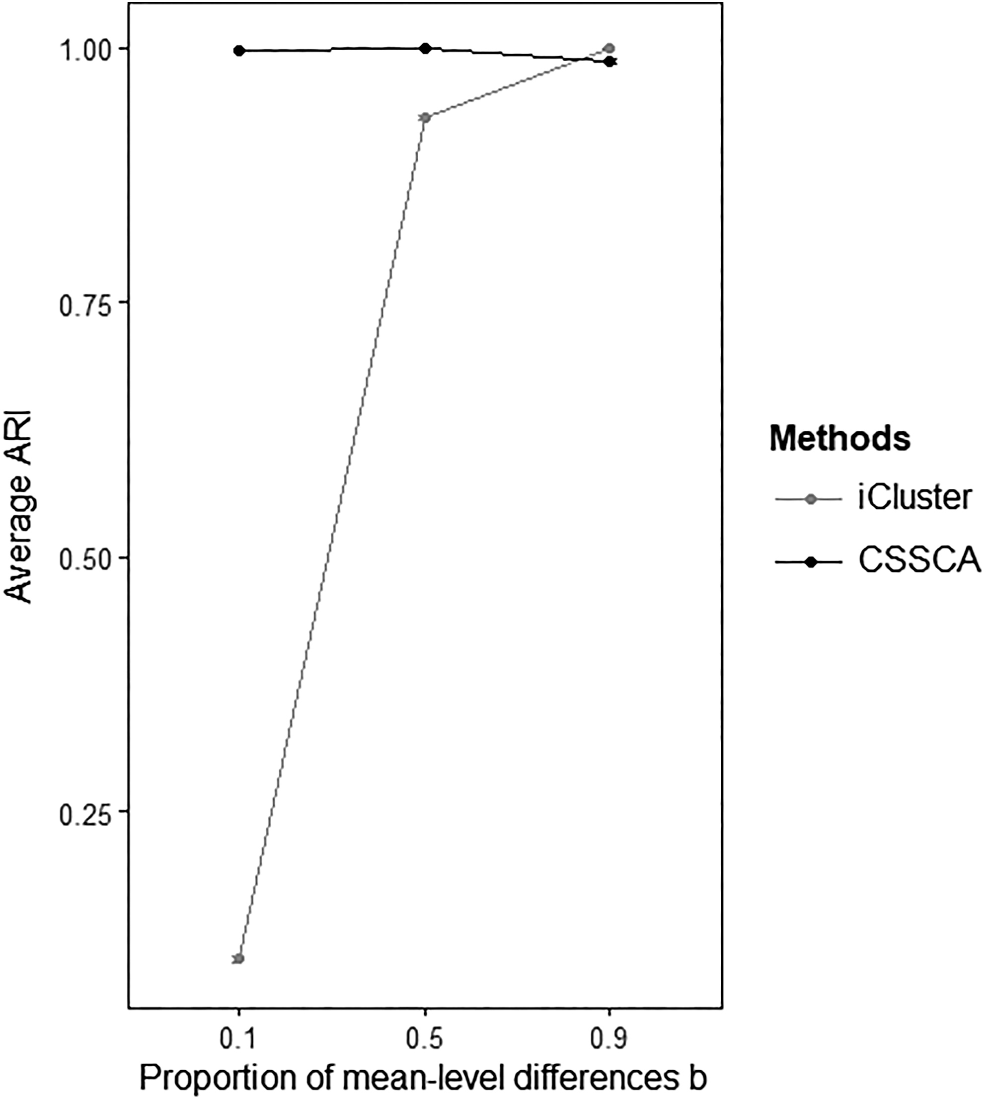
The means and the 95% confidence intervals of the Adjusted Rand Index between the true cluster partitions and the recovered cluster partitions of CSSCA and iCluster in various conditions with different proportions of the mean-level cluster differences (i.e., b).

Recovery of Cluster-Specific Loading Matrices

We also measured the correspondence between the estimated cluster-specific loading matrices and the true loading matrices that were used to generate the data, which we quantified by the goodness-of-cluster-loading-recovery statistic (GOCL; see De Roover et al., 2013). GOCL was calculated by first obtaining Tucker’s congruence coefficients between the corresponding components of the true and estimated loading matrices and then averaging across all components and clusters. Since iCluster only detects mean-level cluster differences, GOCL is not available for the iCluster results.

With an average GOCL equaling 0.95 over all datasets, CSSCA appeared to perform very well in recovering the cluster-specific loading matrices. Since the recovery of the loading matrices largely depends on the recovery of the cluster partitions, we would expect the factors b and e to be also important in predicting CSSCA’s performance in recovering the cluster-specific loading matrices. A cross-tabulation of the average GOCL in function of these two factors is presented in Table 2. Similarly, the average GOCL reaches its lowest value (GOCL = 0.745) for the combination of a large b and large e, that is, the condition where the true component structure is severely masked by the noise.

Table 2.

The Means and the Standard Deviations (in Brackets) of GOCL Between the True Loading Matrices and the CSSCA-Recovered Loading Matrices in Various Conditions.

Noise Level	Proportion of Mean-Level Differences: Low (b = .1)	Proportion of Mean-Level Differences: Medium (b = .5)	Proportion of Mean-Level Differences: High (b = .9)
Low (e = .1)	.99 (.02)	.99 (.01)	.96 (.03)
Medium (e = .2)	.99 (.02)	.98 (.02)	.89 (.06)
High (e = .3)	.98 (.02)	.97 (.03)	.77 (.11)

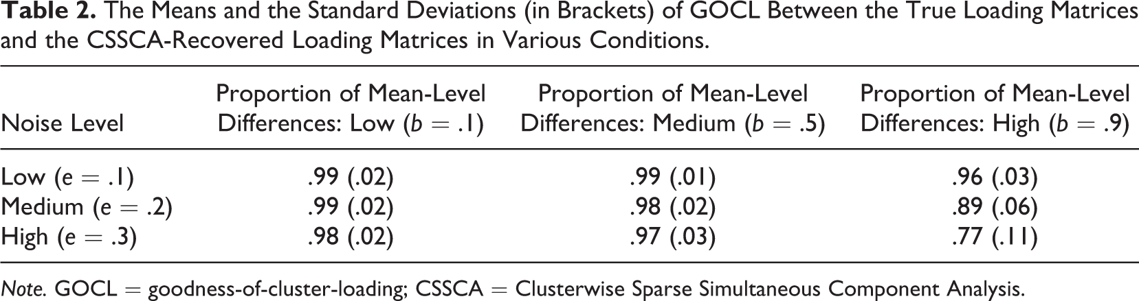
Note. GOCL = goodness-of-cluster-loading; CSSCA = Clusterwise Sparse Simultaneous Component Analysis.

Simulation Study 2

We evaluated the accuracy of the model selection procedure in Simulation Study 2. From Simulation Study 1, it was clear that the two most influential factors of CSSCA performance were (1) the proportion of mean-level cluster differences b and (2) the error level e. Both factors were retained in Simulation Study 2 (note that in Simulation 2, the factor e has two levels: e = .15 or .3). Since the level of sparsity S and the number of clusters K will be selected, they have also been added as manipulated factors in Simulation Study 2. The true level of sparsity S_true is either 3 or 7, and the true number of cluster K_true is either 2 or 4. In total, 576 datasets were created. We executed the model selection procedure for all datasets with K being selected from [1, 2, 3, 4, 5, 6, 7] and S from [0.2, 0.3, 0.4, 0.5, 0.6, 0.7, 0.8]. Over all 576 datasets, both K_true and S_true were correctly selected in 194 datasets (33.68%). In 298 datasets (51.73%), only K_true (but not S_true) was correctly selected, while in 14 datasets (2.43%), only S_true (but not K_true) was correct. Overall, the proposed model selection procedure performed reasonably well in recovering the number of clusters (K_true was successfully recovered in 492, or 85.42%, of the datasets). The model selection procedure was less successful in determining the level of sparsity, where it only succeeded for a total of 208 datasets (36.11%). It is important to note, however, that in most cases the selected level of sparsity differed from the actual level only by a small margin of 0.1. Concerning the two factors, we discovered that model selection of CSSCA was more successful (with respect to selecting both parameters correctly) when (1) b was small to medium size (46.35% when b = .1 vs. 47.40% when b = .5 vs. 7.29% when b = .9) and (2) e was small (36.10% vs. 31.25%). The condition with a large proportion of mean-level cluster differences (i.e., b = .9) and a high level of noise (i.e., e = .3) again was the most difficult condition.

Application

To demonstrate the usefulness of CSSCA, we present an analysis of personality data from Dufner, Arslan, Hagemeyer, Schönbrodt, and Denissen (2015). As part of a large-scale investigation on motive dispositions, the multi-block data—consisting of a total of 171 subjects—contained one block of self-reported scores on motive dispositions and one block of observers’ ratings on participants’ nonverbal behavior in dyadic interviews. The first data block contained a total of six sum-scores of the self-reported scales and three of them indicated the power motive, while the other three indicated the affiliation motive. The second data block includes observers’ ratings on participants’ 18 types of videotaped nonverbal behaviors (see Table 3 for a full list of coded behaviors). A detailed description of the procedures and measurements is available in Hagemeyer, Dufner, and Denissen (2016).

Table 3.

The Loading Matrices of the Common Component for the Three Detected Clusters in the Personality Dataset.

Name of variables	Cluster 1 (N₁ = 68)		Cluster 2 (N₂ = 58)		Cluster 3 (N₃ = 45)
Name of variables	Component 1	Component 2	Component 1	Component 2	Component 1	Component 2
Explicit power motive XMS	0	0	−.19	−.10	.21	−.10
Explicit power motive PRF	−.31	0	−.17	0	.21	0
Explicit power motive UMS	−.20	.12	−.19	0	.21	0
Explicit affiliation motive XMS	.27	0	−.15	0	0	.18
Explicit affiliation motive PRF	0	−.28	−.21	.18	−.11	.47
Explicit affiliation motive UMS	0	−.27	−.13	.20	−.18	.48
Wiggle	0	−.30	0	0	0	0
Overall gesture	0	−.44	−.37	0	0	0
Brash gesture	0	−.42	−.40	0	0	0
Gaze oriented to an experimenter	.30	−.21	−.18	.17	.35	0
Nod	.41	−.24	0	0	.13	.11
Shakes head	0	−.28	0	.13	0	0
Smile	0	0	0	.31	0	0
Friendly laugh	−.22	0	0	.42	0	.18
Relaxed voice	−.24	0	.40	.18	.16	0
Loud voice	−.39	0	0	.09	.11	−.10
Interrupts experimenter	−.35	−.60	0	0	.15	0
Tries to create a pleasant atmosphere	0	0	0	.56	0	.28
Mentions other persons	0	0	.18	0	.29	.54
Behaves friendly	0	0	0	.50	0	.27
Tries to dominate the conversation	−.40	−.29	−.18	0	.49	0
Boasts	−.14	−.17	0	0	.62	−.17
Appears self-secure	−.35	−.21	0	.18	.40	0
Touches self	0	−.17	−.26	0	0	0

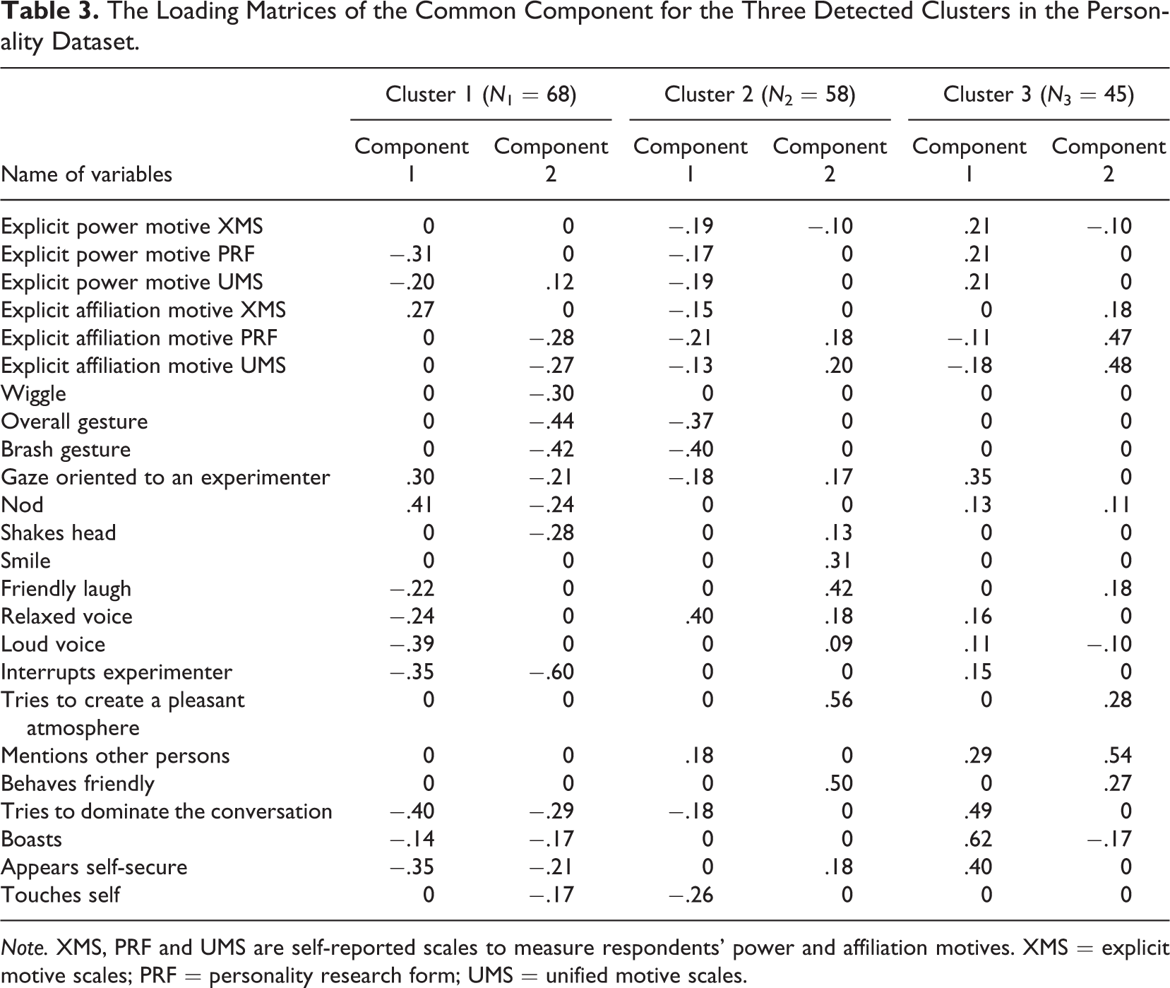
Note. XMS, PRF and UMS are self-reported scales to measure respondents' power and affiliation motives. XMS = explicit motive scales; PRF = personality research form; UMS = unified motive scales.

Our analysis attempted to explore the association between motive dispositions and nonverbal behaviors and to detect subgroup differences therein. Previous studies that tried to reveal the connections between the nonverbal behaviors and the two types of motives drew inconclusive and even contradictory results (see Hall, Coats, & LeBeau, 2005, for a meta-analysis), probably because of the oftentimes ambiguous meanings of nonverbal behaviors (e.g., Vrij, Granhag, & Porter, 2010). We postulate that such contradictory findings might hint at the existence of subgroups, since people belonging to different subgroups may exhibit different nonverbal behaviors as the expressions of their motives.

We performed CSSCA on the multi-block data that consisted of the self-reported scores on motive dispositions and the records of nonverbal behaviors. The multi-block data were column-wise centered and rescaled such that the sum of squares of each variable equaled 1. To choose the appropriate model, the proposed model selection procedure was used with the number of clusters selected from 1, 2,…, 8 and the level of sparsity from 0.1, 0.2,…, 0.9. Furthermore, we fixed the number of common components at two (i.e., the two types of motives), and the number of distinctive components at one per block (i.e., response styles in the first block while specific coding patterns in the second block).

According to the results of the model selection, the average scree ratio achieved its largest value when the number of clusters equaled 3, and, conditional on three clusters, the scree ratio was maximized with the level of sparsity equaling 0.4. We therefore inspected the CSSCA solution with three clusters and 40% of zeros in the loading matrices. The estimated common component loading matrices of the three clusters, which are of particular interest as they imply associations between motive dispositions and nonverbal behaviors, are presented in Table 3.

To illustrate the interpretation of the table, we consider the two common components of Cluster 3. While Component 1 correlates with both power and affiliation motives, Component 2 is primarily related to the affiliation motive, as evidenced by zero or small loadings on the self-reported measurements of the power motive. Component 1 indicates that the following nonverbal behaviors are positively related to the self-reported power motives and meanwhile negatively related to the self-reported affiliation motives: gazing toward the experimenter, mentioning other persons, trying to dominate the conversation, boasting, appearing to be self-secure, nodding, expressing relaxed and loud voice, and interrupting the experimenter. Among these nonverbal behaviors, the first five behaviors appear to be more closely related to the self-reported motives because of their relatively high loadings. In the same vein, the loadings of Component 2 indicate that, for subjects in Cluster 3, the affiliation motive is most strongly related to trying to create a pleasant atmosphere, mentioning other persons and behaving friendly. Moreover, from Table 3, we can also infer that the correlations between the two motives and the nonverbal behaviors are indeed different for different subgroups. For example, although for all three clusters, Component 2 primarily relates to the affiliation motive; it is also clear from the component loadings that the affiliation motive is linked with different sets of nonverbal behaviors for the three clusters, although with large overlap between the sets of Clusters 2 and 3. Overall, the application shows that the CSSCA approach to data analysis can reveal interesting insights in individual differences in the concerted action of attitudinal, emotional, and behavioral indicators.

General Discussion

Applied researchers more and more often make use of multiple blocks of data to obtain insight in complex relations between those factors that influence (social) behavior, often involving novel types of data that consist of a large number of variables. As discussed here, understanding the subtle relations that exist between these influencing factors and their concerted action, in practice means to reveal those variables that covary across data blocks. We also discussed that heterogeneity in such joint influences can be expected, which necessitates the detection of unknown subgroups for which these underlying common sources of variation show up in different sets of linked variables. As argued, to identify unknown clusters and extract cluster-specific linked variables, two challenges of multi-block data analysis should be addressed: (1) High-dimensionality of the data makes the interpretation of the common components infeasible because it concerns an excessive amount of variables, and (2) multi-block data might include distinctive variation underlying one or a few data blocks, which should be set apart from the common variation.

In this article, we introduced CSSCA as a novel clustering method for multi-block data analysis. This method not only accounts for mean-level cluster differences but also for differences in the covariance structure. Furthermore, the two aforementioned challenges are tackled by performing automatic variable selection and by modeling both distinctive and common variation with the distinctive and common components. CSSCA partitions the subjects in such a way that subjects belonging to the same cluster possess the same set of components and means. Through extensive simulations, CSSCA consistently delivered convincing results in recovering clusters and component structures across various conditions. More importantly, CSSCA clearly outperformed iCluster, a popular mean-level clustering method, when substantial cluster differences in the component structure were present in the datasets. We further proposed and verified a model selection procedure to select the number of clusters and level of sparsity. Last, we demonstrated in our illustrative analysis how CSSCA could be applied to exploratory personality psychology research and how such an analysis could bring about novel insights. Concerning the application of CSSCA, we would like to stress that we expect CSSCA to also perform well in analyzing datasets with a large number of subjects (e.g., social network data), despite not formally tested in the current article. This is because with large cluster size, the cluster-specific components could probably be estimated more accurately; as a result, in each update, the subject has a better chance to be assigned to its corresponding cluster.

We propose several future directions for CSSCA. First, we believe that the optimization procedure and the implementation of CSSCA could still be improved to speed up the CSSCA analysis even more. This is especially important when dealing with datasets with large sizes. Second, we found that CSSCA was slightly less accurate and stable in comparison to iCluster when cluster differences mainly pertained to mean-level differences. Future research could, therefore, seek to discover a model selection procedure to determine whether cluster differences are mainly differences in the component structure or differences in the mean structure. If latter is the case, one could instead apply iCluster to obtain even more accurate partitions.

Although the current model selection procedure allows a data-driven selection of the number of clusters and the level of sparsity, to successfully implement CSSCA, researchers are still required to specify the number of common and distinctive components a priori. Nevertheless, further incorporation of component selection tools could surely offer more freedom in the analysis. We refer to two approaches that have been proposed and validated in the existing literature to select the pattern of the components in SCA-based methods (see Gu & Van Deun, 2019, for technical details). The first approach detects the number of total components with the variance accounted for (VAF) method while determines the status (i.e., common or distinctive) of each component with the DISCO-SCA method. The second approach, the principal component analysis - general component analysis (PCA–GCA) method (Smilde et al., 2017), first applies PCA to determine the number of components in each data block and then applies GCA to determine the number of common components.

The current version of CSSCA can only deal with continuous data without missing values. Future research could extend the CSSCA framework to analyze categorical and mixed data types and to handle the missing values (Stacklies et al., 2007).

Last, the proposed model selection procedure, by design, prohibits the selection of the smallest candidate number of clusters and level of sparsity. As a result, the solution of one cluster (i.e., no subgroups exist) and (or) that of nonsparse loading matrices can never be selected. Not being able to select a one-cluster solution is actually a well-known problem of many deterministic clustering methods (Milligan, 1996). Some remedies have been provided to solve this issue, for instance, the lower-bound technique in the context of K-means clustering (Steinley & Brusco, 2011). We encourage future research to address this drawback of CSSCA.

Footnotes

Authors' Note

The authors thank the editor and the anonymous reviewers for providing helpful comments on earlier drafts of the article. Michael Dufner is now affiliated with Medical School Berlin, Germany.

Data Availability

The data used in the simulation can be reproduced by running the simulation R script that is available at under the section Simulation. The application data (i.e., personality data) are available on request from Jaap J. A. Denissen (jjadenissen@gmail.com).

Declaration of Conflicting Interests

The authors declared no potential conflicts of interest with respect to the research, authorship, and/or publication of this article.

Funding

The authors disclosed receipt of the following financial support for the research, authorship, and/or publication of this article: This research was funded by a personal grant from The Netherlands Organization for Scientific Research [NWO-Research Talent 406.17.526] awarded to Shuai Yuan.

Software Information

The simulation and the empirical were conducted using the R software for statistical computing. The scripts of the analysis are available at . There, users can also freely download the R package ClusterSSCA, which implements the CSSCA algorithm.

Supplemental Material

The online supplement to the article is available on PsychArchives at the following address

References

Cadima

Jolliffe

I. T.

(1995). Loading and correlations in the interpretation of principle compenents. Journal of Applied Statistics, 22, 203–214.

Chawarska

Shic

Chen

(2016). Multilevel differences in spontaneous social attention in toddlers with autism spectrum disorder. Child development, 87, 543–557.

De Roover

Timmerman

M. E.

Mesquita

Ceulemans

(2013). Common and cluster-specific simultaneous component analysis. PLoS One, 8, e62280.

Dufner

Arslan

R. C.

Hagemeyer

Schönbrodt

F. D.

Denissen

J. J.

(2015). Affective contingencies in the affiliative domain: Physiological assessment, associations with the affiliation motive, and prediction of behavior. Journal of Personality and Social Psychology, 109, 662.

Fan

Han

Liu

. (2014). Challenges of big data analysis. National Science Review, 1, 293–314.

Gil de Zuniga

Diehl

(2017). Citizenship, social media, and big data: Current and future research in the social sciences. Social Science Computer Review, 35, 3–9.

Van Deun

(2019). RegularizedSCA: Regularized simultaneous component analysis of multiblock data in R. Behavior Research Methods, 51, 2268–2289.

Hagemeyer

Dufner

Denissen

J. J.

(2016). Double dissociation between implicit and explicit affiliative motives: A closer look at socializing behavior in dyadic interactions. Journal of Research in Personality, 65, 89–93.

Hall

J. A.

Coats

E. J.

LeBeau

L. S

. (2005). Nonverbal behavior and the vertical dimension of social relations: A meta-analysis. Psychological Bulletin, 131, 898.

10.

Harzing

A. W.

(2006). Response styles in cross-national survey research: A 26-country study. International Journal of Cross Cultural Management, 6, 243–266.

11.

Haven

ten Berge

J. M. F

. (1977). Tucker’s coefficient of congruence as a measure of factorial invariance: An empirical study. Unpublished manuscript, University of Groningen, Groningen, the Netherlands.

12.

Hellton

K. H.

Thoresen

(2016). Integrative clustering of high-dimensional data with joint and individual clusters. Biostatistics, 17, 537–548.

13.

Hofferth

S. L.

Moran

E. F.

Entwisle

Aber

J. L.

Brady

H. E.

Conley

… Hubacek

. (2017). Introduction: History and motivation. Annals of the American Academy of Political and Social Science, 669, 6–17.

14.

Hubert

Arabie

(1985). Comparing partitions. Journal of Classification, 2, 193–218.

15.

Jolliffe

. (2011). Principal component analysis (pp. 1094–1096). Berlin, Germany: Springer.

16.

Jung

Wickrama

K. A. S.

(2008). An introduction to latent class growth analysis and growth mixture modeling. Social and Personality Psychology Compass, 2, 302–317.

17.

Kiers

H. A.

ten Berge

J. M.

(1989). Alternating least squares algorithms for simultaneous components analysis with equal component weight matrices in two or more populations. Psychometrika, 54, 467–473.

18.

Lock

E. F.

Hoadley

K. A.

Marron

J. S.

Nobel

A. B

. (2013). Joint and individual variation explained (JIVE) for integrated analysis of multiple data types. The Annals of Applied Statistics, 7, 523.

19.

Meredith

Millsap

R. E

. (1985). On component analyses. Psychometrika, 50, 495–507.

20.

Milligan

G. W.

(1996). Clustering validation: results and implications for applied analyses. In Arabie

Hubert

L. J.

De Soete

(Eds.), Clustering and classification (pp. 341–375). London, UK: World Scientific.

21.

Sandri

B. J.

Kaplan

Hodgson

S. W.

Peterson

Avdulov

Higgins

… Bitterman

(2018). Multi-omic molecular profiling of lung cancer in COPD. European Respiratory Journal, 52, 1702665.

22.

Schouteden

Van Deun

Pattyn

Van Mechelen

(2013). SCA with rotation to distinguish common and distinctive information in linked data. Behavior Research Methods, 45, 822–833.

23.

Shen

Olshen

A. B.

Ladanyi

(2009). Integrative clustering of multiple genomic data types using a joint latent variable model with application to breast and lung cancer subtype analysis. Bioinformatics, 25, 2906–2912.

24.

Smilde

A. K.

Måge

Naes

Hankemeier

Lips

M. A.

Kiers

H. A. L.

… Bro

(2017). Common and distinct components in data fusion. Journal of Chemometrics, 31, e2900.

25.

Stacklies

Redestig

Scholz

Walther

Selbig

(2007). pcaMethods—a bioconductor package providing PCA methods for incomplete data. Bioinformatics, 23, 1164–1167.

26.

Steinley

(2004). Properties of the Hubert-Arable Adjusted Rand Index. Psychological Methods, 9, 386.

27.

Steinley

Brusco

M. J.

(2011). Choosing the number of clusters in K-means clustering. Psychological Methods, 16, 285.

28.

Stute

Zhu

L. X.

(1995). Asymptotics of k-means clustering based on projection pursuit. Sankhyā: The Indian Journal of Statistics, Series A, 462–471.

29.

Tenenhaus

(2014). Regularized generalized canonical correlation analysis for multiblock or multigroup data analysis. European Journal of Operational Research, 238, 391–403.

30.

Timmerman

M. E.

Ceulemans

De Roover

Van Leeuwen

(2013). Subspace K-means clustering. Behavior Research Methods, 45, 1011–1023.

31.

Timmerman

M. E.

Kiers

H. A.

(2003). Four simultaneous component models for the analysis of multivariate time series from more than one subject to model intraindividual and interindividual differences. Psychometrika, 68, 105–121.

32.

Tucker

L. R

. (1951). A method for synthesis of factor analysis studies (No. PRS-984). Princeton, NJ: Education Testing Service.

33.

Van Deun

Smilde

A. K.

van der Werf

M. J.

Kiers

H. A.

Van Mechelen

. (2009). A structured overview of simultaneous component based data integration. BMC Bioinformatics, 10, 246.

34.

Van Deun

Wilderjans

T. F.

Van den Berg

R. A.

Antoniadis

Van Mechelen

. (2011). A flexible framework for sparse simultaneous component based data integration. BMC Bioinformatics, 12, 448.

35.

Vargo

C. J.

Hopp

(2017). Socioeconomic status, social capital, and partisan polarity as predictors of political incivility on twitter: A congressional district-level analysis. Social Science Computer Review, 35, 10–32.

36.

Vichi

Kiers

H. A.

(2001). Factorial k-means analysis for two-way data. Computational Statistics & Data Analysis, 37, 49–64.

37.

Vrij

Granhag

P. A.

Porter

(2010). Pitfalls and opportunities in nonverbal and verbal lie detection. Psychological Science in the Public Interest, 11, 89–121.

38.

Waldherr

Maier

Miltner

Günther

(2017). Big data, big noise: The challenge of finding issue networks on the web. Social Science Computer Review, 35, 427–443.

39.

Wang

(2016). Integrative clustering methods of multi-omics data for molecule-based cancer classifications. Quantitative Biology, 4, 58–67.

40.

Wells

Thorson

(2017). Combining big data and survey techniques to model effects of political content flows in Facebook. Social Science Computer Review, 35, 33–52.

41.

Wilderjans

T. F.

Ceulemans

(2013). Clusterwise Parafac to identify heterogeneity in three-way data. Chemometrics and Intelligent Laboratory Systems, 129, 87–97.

42.

Wang

Zhang

M. Q.

(2015). Fast dimension reduction and integrative clustering of multi-omics data using low-rank approximation: Application to cancer molecular classification. BMC Genomics, 16, 1022.

43.

Risk

B. B.

Zhang

Marron

J. S.

(2017). JIVE integration of imaging and behavioral data. NeuroImage, 152, 38–49.

44.

Zou

Hastie

Tibshirani

. (2006). Sparse principal component analysis. Journal of Computational and Graphical Statistics, 15, 265–286.

Revealing Subgroups That Differ in Common and Distinctive Variation in Multi-Block Data: Clusterwise Sparse Simultaneous Component Analysis

Abstract

Keywords

Introduction

Method

Multi-Block Data

SCA

SSCA With Common and Distinctive Components

CSSCA

Model and Objective Function

Related Methods

Algorithm and Model Selection

Algorithm

Model Selection

Simulation Studies

Simulation Study 1

Design

Results and Discussion

Execution Time of CSSCA

Clustering Accuracy of CSSCA

Comparison of CSSCA and iCluster in Clustering Accuracy

Recovery of Cluster-Specific Loading Matrices

Simulation Study 2

Application

General Discussion

Footnotes

Authors' Note

Data Availability

Declaration of Conflicting Interests

Funding

Software Information

Supplemental Material

References