Sage Journals: Discover world-class research

Abstract

This article addresses the questions of whether paradata can help us to improve the models of panel attrition and whether paradata can improve the effectiveness of propensity score weights with respect to reducing attrition biases. The main advantage of paradata is that it is collected as a by-product of the survey process. However, it is still an open question which paradata can be used to model attrition and to what extent these paradata are correlated with the variables of interest. Our analysis used data from a seven-wave web-based panel survey that had been supplemented by three cross-sectional surveys. This split panel design allowed us to assess the magnitude of attrition bias for a large number of substantive variables. Furthermore, this design enabled us to analyze in detail the effectiveness of propensity score weights. Our results showed that some paradata (e.g., response times and participation history) improved the prediction of panel attrition, whereas others did not. In addition, not all the paradata that increased the model fit resulted in weights that effectively reduced bias. These findings highlight the importance of selecting paradata that are linked to both the survey response process and the variables of interest. This article provides a first contribution to this challenge.

Keywords

panel attrition paradata propensity score weighting nonresponse bias

Introduction

Within the last decades, panel surveys have become more and more popular in social science research, and their number has increased substantially (Andreß, Golsch, & Schmidt, 2013). Thereby, they are “fast displacing their cross-sectional counterpart at the heart of sociological research” (Halaby, 2004, p. 507). The success of panel surveys can be attributed to their manifold analytical advantages. Among others, they allow researchers to measure change at the individual level, to separate age from cohort effects, and to assess measurement errors (Andreß et al., 2013; Firebaugh, 2008). Most importantly, panel data enable us to control for the effects of unobserved variables and, thus, to estimate causal effects (Andreß et al., 2013; Firebaugh, 2008; Halaby, 2004). Notwithstanding, panel surveys suffer from several drawbacks. One of the most important concerns about panel surveys is panel attrition (Lynn, 2009). When conducting a panel survey, researchers inevitably confront the problem of nonresponding sample members over the course of consecutive waves of the survey. Unit nonresponse in a reinterview may be caused by various factors such as mortality, nonavailability, and refusals (Watson & Wooden, 2009, pp. 159–167). However, if a variable of interest is correlated with the response propensity of respondents, this correlation constitutes a bias in the variable of interest (Bethlehem, 2002; Groves, 2006). A bias in estimates is a threat to the inferences we draw from survey data. Thus, methods to correct for biases have been proposed. Among others, these include methods to impute the missing cases (Rubin, 1987) or to weight the remaining cases by their response propensity (Rosenbaum & Rubin, 1983). The latter method is often referred to as propensity score weighting. In this article, we focus on weighting methods as they are frequently used to deal with panel attrition. Their popularity relies on the beneficial property that they are easy to provide for data collections and easy to apply in statistical analyses by users employing standard statistical software tools.

Propensity score weighting is based on the idea of modeling the response process to yield estimates of the response propensities. Then, the inverse of these response propensities is used as weights, which can correct for existing attrition biases. However, research has shown that propensity score weighting does not eliminate all of the existing biases (Bergmann, 2011; Blumenstiel & Gummer, 2015; Vandecasteele & Debels, 2007). In certain situations, propensity score weighting even increases the existing biases. As Kreuter and Olson (2011) have shown, this undesirable outcome can be attributed to imperfectly specified models, which lack the relevant variables or inadequately represent the survey response process. The capability of propensity score weights to correct for biases crucially depends on how well the variables in the underlying model are correlated with the response propensity, as well as the variables of interest (Kreuter & Olson, 2011; Little & Vartivarian, 2005). Thus, it is of pivotal importance to carefully select the variables to be included in the models to predict panel attrition. However, a standard set of variables that fits this purpose hasn’t been developed yet. Although some excellent approaches exist that provide us with models of the response process (Groves et al., 2009; Lepkowski & Couper, 2002; Watson & Wooden, 2009), we have found a multitude of studies on panel attrition and propensity score weighting that use a variety of different explanation models (e.g., Blumenstiel & Gummer, 2015; Kroh & Spieß, 2008; Vandecasteele & Debels, 2007). Consequently, there is still a remarkable shortage of variables that can be used to predict panel attrition and to correct for biases. That being said, improving model selection is a vital challenge for survey research.

The recent rise of paradata in data collection promises to remedy at least some of the issues identified by this challenge. Paradata, collected as a by-product of the survey process (Couper, 2000), encompass data that describe the process of responding, for example, response latencies, response patterns (e.g., counts of missing items), and information on the device a respondent used to answer the questionnaire (cf. Callegaro, 2013; Couper, 2000). Paradata are particularly easy to collect when using computer-assisted data collection modes, for instance, web surveys (e.g., Stieger & Reips, 2010). Therefore, they are an easily available and cost-efficient alternative to other auxiliary data. Further advantages are that paradata are usually not consciously provided by respondents, are available at the level of the individual, and can be abstracted and aggregated to more general and meaningful information (Kaczmirek, 2008, p. 60). Consequently, paradata are increasingly used to study various issues in survey methodology, for instance, to detect what devices respondents use to answer web surveys and how they navigate through the questionnaires (Callegaro, 2013), in the analyses of response latencies (Couper & Kreuter, 2013; Heerwegh, 2003), interview duration (Gummer & Roßmann, 2015), nonresponse adjustment (Biemer, Chen, & Wang, 2013; Sinibaldi, Trappmann, & Kreuter, 2014), visual layout (Stern, 2008), within-survey requests (Sakshaug, 2013), and data collection in general (Kreuter, Couper, & Lyberg, 2010). The question arises as to whether paradata can improve our understanding of unit nonresponse and, hence, panel attrition bias (e.g., Kreuter & Olson, 2013; Sinibaldi et al., 2014). Considering the beneficial properties of paradata and their promising potential for methodological applications, this article aims to answer the following two main research questions:

First, can paradata successfully be applied to improve the prediction of attrition in panel surveys? If this proves to be true, the second question directly emerges from the first one: Do corresponding propensity score weights also improve the correction of panel attrition bias in variables of interest?

By shedding light on the relationship between paradata, unit nonresponse, and bias, this article addresses two major shortcomings in the current literature. First, we provide evidence about which paradata are worthwhile to consider for data collection and for the assessment of data quality with respect to unit nonresponse bias. Second, our findings contribute to the development of a collection of variables for which empirical evidence exists that they contribute to predicting panel attrition and correcting for biases. The establishment of such a tool kit and a continuous extension of it with new empirical evidence from different data collection modes, panel survey designs, and contexts would constitute a huge advance in survey methodology, since it would enable researchers and practitioners to assess and correct panel attrition more efficiently.

In the next two sections, we introduce our data and methods. The following section presents the results of our analyses and provides answers to our research questions. Finally, we discuss our findings and provide some suggestions for further research opportunities.

Data

To answer our research questions, we used data from a seven-wave web-based panel survey. This survey, which covered the 2013 German election campaign as part of the German Longitudinal Election Study (Rattinger, Roßteutscher, Schmitt-Beck, Weßels, & Wolf, 2014), was conducted from June to October 2013. The survey questionnaires included sociodemographics and a broad set of questions on political attitudes and behavior. The initial sample of 5,256 respondents was drawn from one of the largest German online access panels of around 96,000 active panelists by using quotas on gender, age, and education. As part of the sample, a group of 1,011 respondents were selected because they already had participated in an antecessor panel survey of the 2009 German election.

The panel survey was designed as a split panel (G. J. Duncan & Kalton, 1987) supplemented by three cross-sectional web surveys as shown in Figure 1. Each of these cross-sectional surveys parallels their respective panel survey waves and consists of a sample of about 1,200 respondents each. The questionnaires of the cross-sectional surveys were the same as for the panel waves except for an additional sociodemographic part at the end of the cross-sectional surveys. Hence, the cross-sectional surveys and the corresponding panel waves are comparable on the item level. To further enhance comparability, the samples of the cross-sectional surveys were drawn from the same online access panel using the same quotas.

Figure 1.

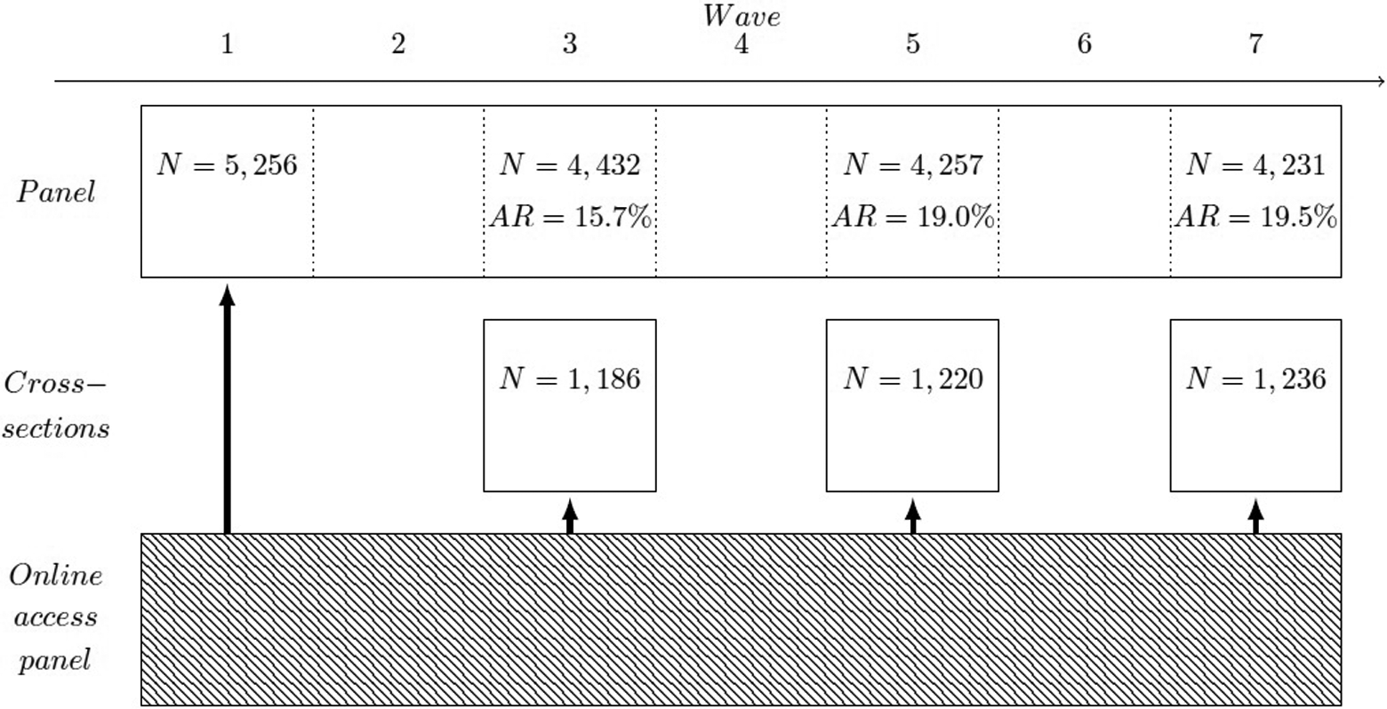
Schematic of the web-based panel survey and the supplemental cross-sectional surveys.

On average, it took a respondent 23 min to complete a single questionnaire for the panel survey. The average interview duration for the cross-sectional surveys was slightly higher (about 28 min).¹

The application of a split panel design allows us to estimate the bias due to panel attrition by comparing the panel waves to the cross-sectional surveys at the item level. The major advantage of this design is that we can measure bias with reference to a large quantity of substantive variables of interest. Furthermore, we can also analyze how far propensity score weights are able to reduce panel attrition biases.

Participation in a panel wave was coded as a dummy variable (0 = nonparticipation/1 = participation). We used these dummy variables as dependent variables in our analyses. Figure 1 shows the number of respondents for each wave and the rate of attrition calculated on the basis of the initial sample. Each respondent who completed the initial Wave 1 was contacted to be reinterviewed in subsequent waves, irrespective of whether he or she missed some of the waves.

To predict participation in a panel wave, we used a set of sociodemographic and substantive variables. We selected variables that had been used in prior work on nonresponse/attrition (e.g., Blumenstiel & Gummer, 2015; Fricker & Tourangeau, 2010; Kroh & Spieß, 2008; Vandecasteele & Debels, 2007) or related to theoretical dimensions of nonresponse (cf. Groves et al., 2009; Lepkowski & Couper, 2002; Watson & Wooden, 2009). Descriptive statistics for all dependent and independent variables of our nonresponse models are given in Table 1.

Table 1.

Variables Used in the Analytical Scenarios.

Variables	Scale/Coding	Mean (SD)	S1	S2	S3
Dependent Variables
Participation in Wave 3	0/1	0.84 (0.36)	x	x	x
Participation in Wave 5	0/1	0.81 (0.39)	x	x	x
Participation in Wave 7	0/1	0.80 (0.40)	x	x	x
Independent variables
Age	18–83	45.69 (14.64)	x	x	x
(Age)²	324–6889	2302.38 (1360.68)	x	x	x
Gender: female	0/1	0.51 (0.50)	x	x	x
Education
Low	0/1	0.30 (0.46)	x	x	x
Intermediate	0/1	0.43 (0.49)	x	x	x
High	0/1	0.27 (0.44)	x	x	x
Partner	0/1	0.71 (0.46)	x	x	x
Religiosity	0–4	1.10 (1.17)	x	x	x
Household size	1–8	2.32 (1.16)	x	x	x
Income	1–13	6.29 (2.65)	x	x	x
Region: Eastern Germany	0/1	0.22 (0.41)	x	x	x
Unemployment within last 10 years	0/1	0.35 (0.48)	x	x	x
Employment status
Labor force	0/1	0.77 (0.42)	x	x	x
Retired	0/1	0.17 (0.38)	x	x	x
Housewife	0/1	0.06 (0.24)	x	x	x
Interest in politics	0–4	2.30 (1.03)	x	x	x
Political communication	0/1	0.47 (0.50)	x	x	x
Strength of party identification	0–5	2.61 (1.82)	x	x	x
Satisfaction with democracy	0–4	2.06 (0.94)	x	x	x
Chancellor preference	0/1	0.64 (0.48)	x	x	x
Turnout	0/1	0.85 (0.35)	x	x	x
Political knowledge: politicians and parties	0/1	0.46 (0.50)	x	x	x
Economic knowledge: unemployment rate	0/1	0.32 (0.47)	x	x	x
Big 5: extraversion	Factor score	0.00 (0.83)	x	x	x
Big 5: openness	Factor score	0.00 (0.75)	x	x	x
Big 5: conscientiousness	Factor score	0.00 (0.75)	x	x	x
Big 5: neuroticism	Factor score	0.00 (0.76)	x	x	x
Big 5: agreeableness	Factor score	0.00 (0.73)	x	x	x
Need for cognition	1–5	3.55 (0.72)	x	x	x
Need to evaluate	1–5	3.65 (0.64)	x	x	x
Need for cognitive closure	1–5	3.39 (0.73)	x	x	x
Duty to vote	1–5	4.08 (1.11)	x	x	x
Internal efficacy	Factor score	0.00 (0.85)	x	x	x
External efficacy	Factor score	0.00 (0.79)	x	x	x
Participation due to incentives	0/1	0.25 (0.43)	x	x	x
Survey experience	0–3	1.59 (0.83)	x	x	x
Respondent’s motivation	Factor score	0.00 (0.81)	x	x	x
Membership in different panels	0–5	1.29 (1.57)	x	x	x
(Membership in different panels)²	0–25	4.12 (7.17)	x	x	x
Internet usage in days per week	0–7	6.68 (0.96)	x	x	x
No. of correctly answered control questions	0–2	1.72 (0.57)		x	x
No. of item nonresponses	0–54	2.01 (6.00)		x	x
No. of don’t know answers	0–28	4.34 (5.12)		x	x
Device
Personal computer/notebook	0/1	0.95 (0.23)		x	x
Smartphone	0/1	0.03 (0.16)		x	x
Tablet computer	0/1	0.03 (0.17)		x	x
Response speed index	Index score	1.01 (0.23)		x	x
Participation in 2009 panel survey	0/1	0.19 (0.39)		x	x
No. of completed surveys in last 3 months	0–54	14.53 (7.59)			x

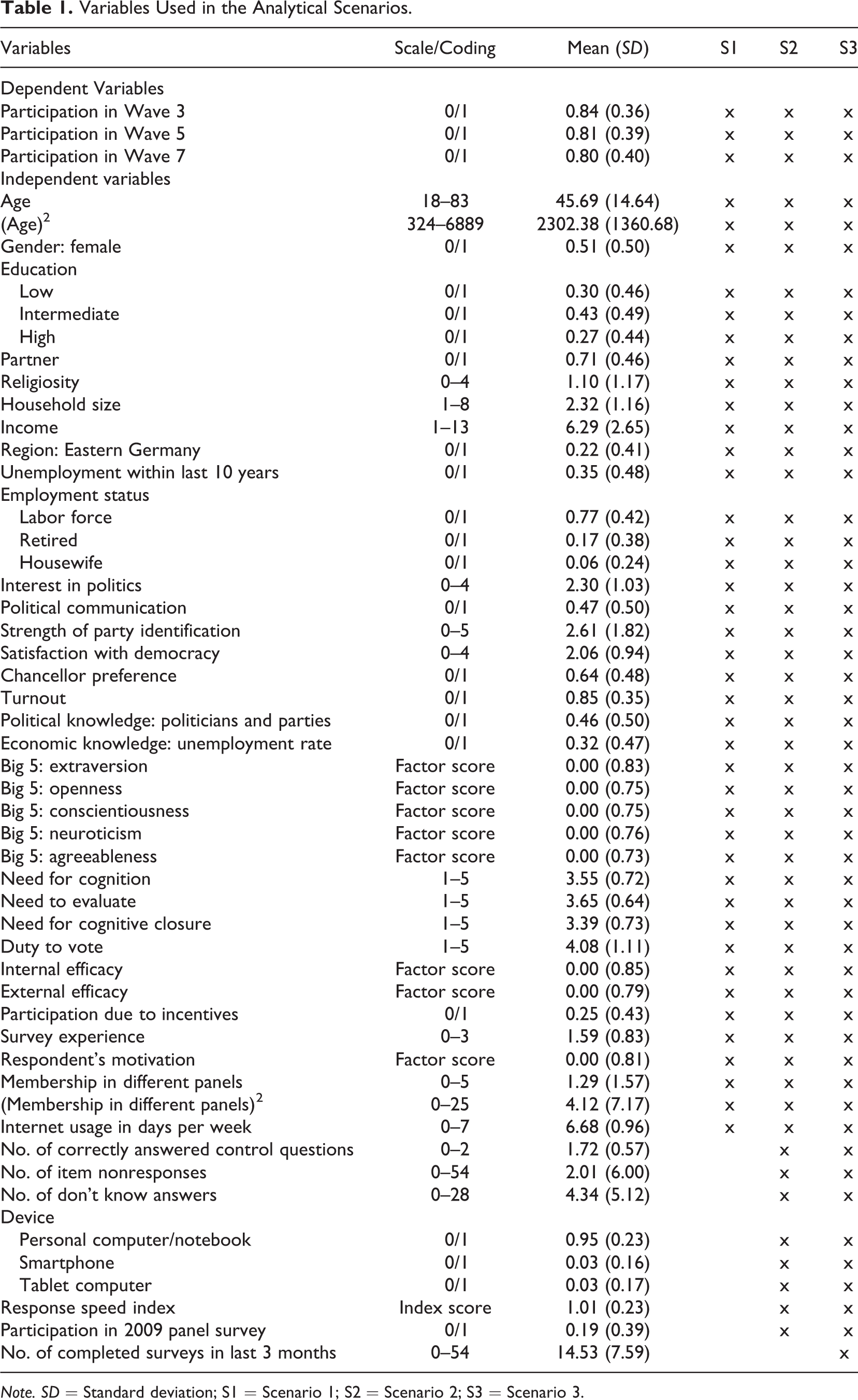
Note. SD = Standard deviation; S1 = Scenario 1; S2 = Scenario 2; S3 = Scenario 3.

To study the potentials of paradata to explain panel attrition and to correct for attrition biases, we collected a set of paradata variables, which include response latencies, measures of response patterns, information on the device used by respondents to answer the survey, and indicators of previous participation in surveys. These paradata variables are widely available, especially—but not in all cases exclusively—in web surveys, and researchers can easily obtain them in most instances. Response latencies can be collected by common survey software, and measures of response patterns usually can be generated during data preparation without a great deal of work. The information on the devices used by respondents is collected in many web survey packages, and indicators of previous participation in surveys are often provided by (online access) panel operators.

First, all panel waves included control questions, which asked respondents to select a specific category of the response scale. We counted the absolute number of correctly answered control questions (0–2) to measure respondents’ attentiveness when completing the survey. Our basic assumption was that attentive respondents are motivated to participate in further panel waves and, at the same time, show optimizing response behavior (Krosnick, 1991, 1999). Since satisficing among inattentive respondents potentially biases substantive variables of interest, we suspected that there might be an interconnection between inattentiveness, responses to variables of interest, and participation in further panel waves.

Second, to measure the propensity of respondents to substantially answer the questions in the survey, we counted the number of item nonresponses and “don’t know” responses to the questionnaire. On the one hand, a high number of item nonresponses can indicate a low response propensity, whereas on the other hand, frequently declining to answer questions or to answer “don’t know” might indicate a low motivation or deficiencies in cognitive abilities (cf. Beatty & Herrmann, 2002; Krosnick, 1991, 1999). Respondents who are low in motivation were shown to have an increased risk of dropping out of web surveys, which also is a form of nonresponse that causes bias in the variables of interest (Roßmann, Blumenstiel, & Steinbrecher, 2014).

Third, we determined the type of device a respondent used to complete the survey by using information from the user agent strings that are commonly collected by web survey software. The Stata module parseuas (Roßmann & Gummer, 2014) was used to code the use of personal computers, tablets, and smartphones. Answering a web survey on a mobile device can be burdensome due to small screen sizes, low Internet connection speed, or an increased number of distractions when using the device in busy environments (De Bruijne & Wijnant, 2013; Mavletova, 2013; Peytchev & Hill, 2010). As a result, when respondents use mobile phones instead of personal computers, their completion rates seem to be lower and their break-off rates higher (Mavletova, 2013). Thus, we assumed that using a mobile device can increase task difficulty, decrease respondents’ motivation, and make participation in consecutive panel waves less likely. In addition, the adoption of mobile technology is not uniform across the population. In the United States, smartphone ownership is highest among those with high incomes, college education, and young adults (Link et al., 2014). Hence, using a mobile device to answer the survey might also be linked to substantive responses to variables of interest. Although recent research has found only limited evidence for the effects of using mobile devices on data quality (Mavletova, 2013) and mean responses to substantive variables (De Bruijne & Wijnant, 2013), we explored whether a link exists between using a mobile device, substantive responses, and panel attrition.

Fourth, response latencies are one of the most widely used forms of paradata (Olson & Parkhurst, 2013). They are commonly interpreted as a measure for the extent of cognitive activity in the response process (cf. Couper & Kreuter, 2013; Yan & Tourangeau, 2008). One theoretical perspective argues that answering questions exceptionally fast is an indication of satisficing response behavior (Callegaro, Yang, Bhola, Dillman, & Chin, 2009; Greszki, Meyer, & Schoen, 2014; Malhotra, 2008; Zhang & Conrad, 2014). Accordingly, a fast response speed indicates that respondents may have a low cognitive ability or low motivation that may affect their propensity to participate and the accuracy of their responses. However, short response times might also reflect highly accessible attitudes (e.g., Bassili, 1993; Fazio, 1990; Fazio, Sanbonmatsu, Powell, & Kardes, 1986) and should be linked to a lower response burden and a higher motivation to participate in further panel waves. In addition, longer response times might also signal problems in answering survey questions (e.g., Bassili & Scott, 1996). Thus, these longer times may indicate a high response burden and are potentially linked to a lower response propensity. To investigate the effects of response times on panel attrition, we computed a response speed index on the basis of page-level response times using the Stata module rspeedindex (Roßmann, 2015).

Fifth, participation in the 2009 panel survey should have encouraged respondents to take part again in the 2013 panel survey. Since the respondents already had decided to participate once, further willingness to participate in a follow-up survey constitutes a consistent behavioral pattern. Hence, these respondents should show a higher likelihood to participate to avoid cognitive dissonance (Festinger, 1957). Yet, only the participants of 2009 who were still part of the online access panel could be invited to participate again. Presumably, the respective group of respondents was highly motivated and inclined to participate in surveys. We used a permanent respondent ID to determine whether a respondent participated in both surveys.

Finally, we used the respondents’ participation history over a certain time period as a measure of the general response propensity, which was a count of the absolute number of surveys a respondent completed within the preceding 3 months. We assumed that a measure of the general response propensity would be an excellent predictor of participation in consecutive panel waves. However, it is important to note that the theoretical link between the respondents’ participation history and the content of variables of interest remains unclear.

Method

To answer both research questions, first, we fitted logistic regressions to model panel attrition in Waves 3, 5, and 7 (i.e., the transitions from Wave 1 to Wave 3, from Wave 1 to Wave 5, and from Wave 1 to Wave 7, respectively). Accordingly, all the models were based on the respondents’ characteristics measured in Wave 1. The rationale for choosing these transitions between waves was that the panel waves were paralleled by the cross-sectional web surveys. To study whether the use of paradata improves the explanation of panel attrition, three different models (scenarios) were used to predict attrition (Table 1).

In the first scenario, we set up a model with an extensive set of sociodemographic characteristics, attitudes, and predispositions of the respondents. These variables were available for all respondents, since they were collected in Wave 1 of the panel survey.

In the second scenario, we extended Scenario 1 with a set of the paradata described previously, which included the number of correctly answered control questions, the number of item nonresponses and “don’t know” responses, the type of device used to answer the survey, the index of the respondents’ average response speed, and participation in the 2009 panel survey.

The third scenario added the respondents’ participation history in the online access panel to the model used in Scenario 2. We assumed that the overall web survey participation behavior of a respondent would be an excellent predictor for participation in a specific survey. However, at the same time, all other variables that explain participation behavior would likely lose explanatory power, since they were correlated with former participation behavior as well. Thus, in comparison to the second scenario, Scenario 3 represents an enhanced model. Although adding a measure of the respondents’ participation history does not advance the theoretical explanation of panel attrition, it will likely boost the fit of the statistical model. In addition, we did not assume that adding this predictor would enhance the correlation between the model of attrition and variables of interest.

The models of the scenarios were then used to predict panel attrition in Waves 3, 5, and 7.² We computed propensity score weights by inverting the predicted response propensities (Horvitz & Thompson, 1952).³ Respondents with a high response propensity had a small weight, whereas respondents with a low propensity had a higher weight. When applying the weights to an analysis, low propensity respondents become more influential compared to respondents with a high response propensity. To sum up, for each of the three transitions, we computed three weights that corresponded to the three analytical scenarios.

To study the effects of including paradata in the calculation of propensity score weights, we compared the results of weighted analyses within each of the three transitions (i.e., from Wave 1 to Wave 3, Wave 1 to Wave 5, and Wave 1 to Wave 7). A comparison of the results for three transitions served as a robustness check. In addition, it allowed us to analyze whether the effectiveness of the weights differed between the transitions.

Using data from a split panel with nearly identical questionnaires enabled us to gauge the initial attrition bias for variables of interest by comparing the distribution of a variable between a panel wave and the parallel cross-sectional survey. In a second step, we assessed the remaining bias after applying propensity score weights by comparing the weighted distribution of a variable in a panel wave to its unweighted distribution in the parallel cross-sectional survey. To measure the effectiveness of weighting, we compared the bias of each variable before and after weighting with the propensity score weights from Scenarios 1–3.

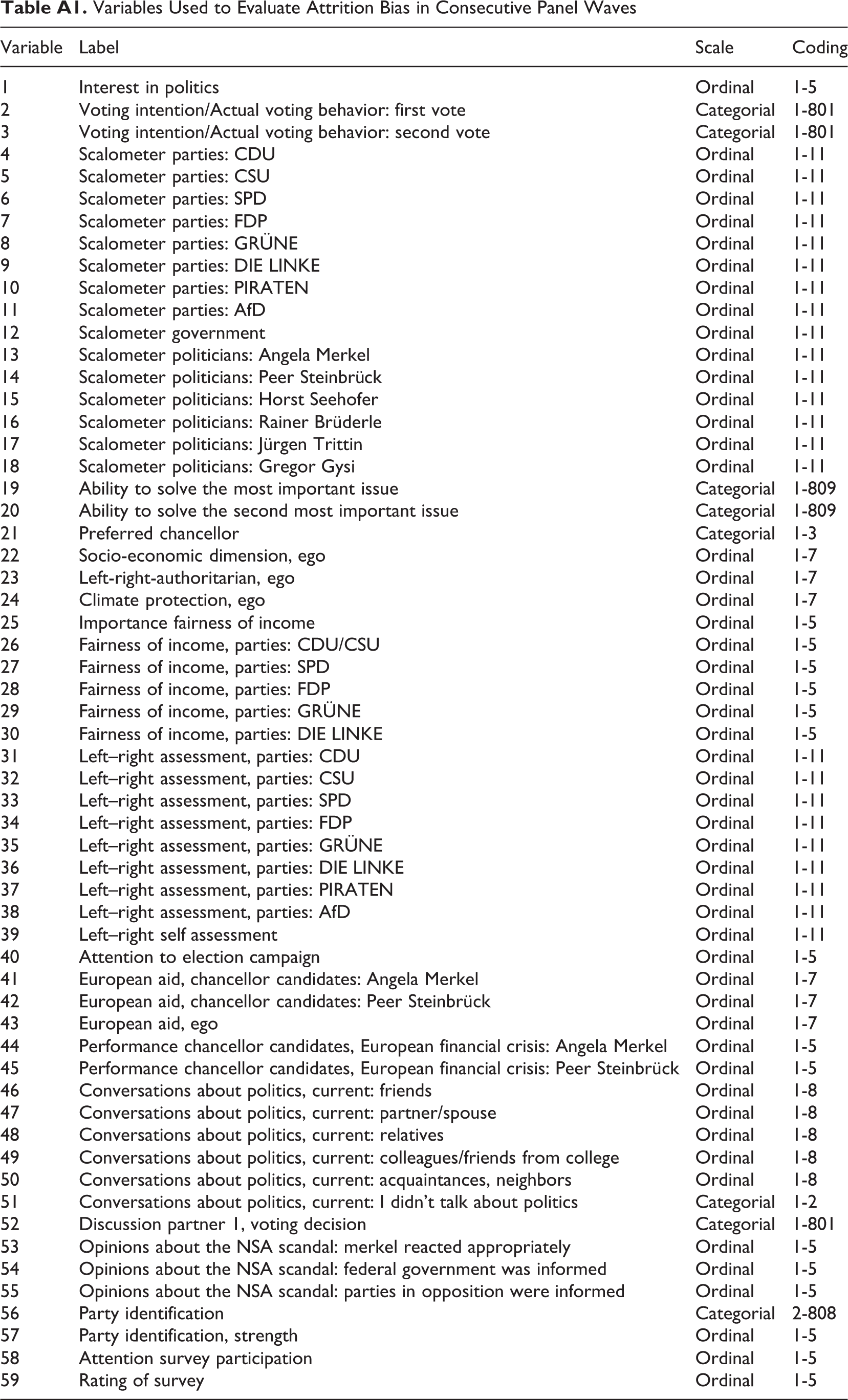
Usually, we only have a very limited number of external references with which to compare the distribution of variables of interest. In addition, especially in large-scale surveys, many variables are of interest to researchers. Therefore, we studied the effectiveness of propensity score weighting based on a comprehensive set of variables, which were asked in each of the three supplemental cross-sectional web surveys (N = 59). Table A1 gives an overview of all of the 59 variables used in the analysis. Yet, the number of variables made it necessary to rely on a comparable indicator of nonresponse bias, which enabled us to calculate averaged indicators of nonresponse for all 59 variables. This strategy enabled us to avoid comparing the marginal distributions of 59 variables without weighting to the three weighting scenarios (i.e., 236 distributions).

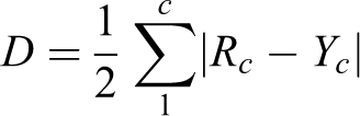
We used dissimilarity indexes (O. D. Duncan & Duncan, 1955) to measure the nonresponse bias of a variable (cf. Blumenstiel & Gummer, 2015). These indexes are used to capture differences between two distributions. In our case, the difference in the distribution between a variable suffering from attrition and the same variable without attrition is what is commonly referred to as nonresponse bias. A dissimilarity index is defined as follows:

D = \frac{1}{2} \sum_{1}^{c} |R_{c} - Y_{c}|

where Y is the relative distribution of the variable of interest in the panel, R is the relative distribution of the variable of interest in the parallel cross-sectional survey, and c is the number of the response categories of the variable of interest. Accordingly, Y_c and R_c are the relative frequencies of category c of a variable in the panel survey and the cross-sectional survey, respectively. We argue that this approach is preferable to other methods such as t-tests, since we can use it independently from a variable’s scaling. Furthermore, it shifts the perspective from mean differences to differences in distributions. For each variable in each wave, we calculated four dissimilarity indexes: bias unweighted, bias after using propensity score weights of Scenario 1, bias after using propensity score weights of Scenario 2 (including paradata), and bias after using propensity score weights of Scenario 3 (including paradata and the respondents’ participation history).

Results

Prediction of Panel Attrition

In the first step, we addressed the question whether paradata can be successfully used to improve the prediction of attrition in web-based panel surveys. Table 2 provides a brief summary of the model fit of the logistic regressions on response in Waves 3, 5, and 7 for each of the three scenarios. We presented the McFadden’s R² statistic as an indicator of model fit.

Table 2.

Model Fit of the Logistic Regressions Used to Predict Response Propensities.

Model	N	McFadden’s R²
Model	N	Wave 3	Wave 5	Wave 7
Scenario 1: baseline model	4,595	0.109	0.101	0.108
Scenario 2: baseline model + paradata	4,595	0.124	0.116	0.122
Scenario 3: baseline model + paradata + participation history	4,595	0.442	0.474	0.421

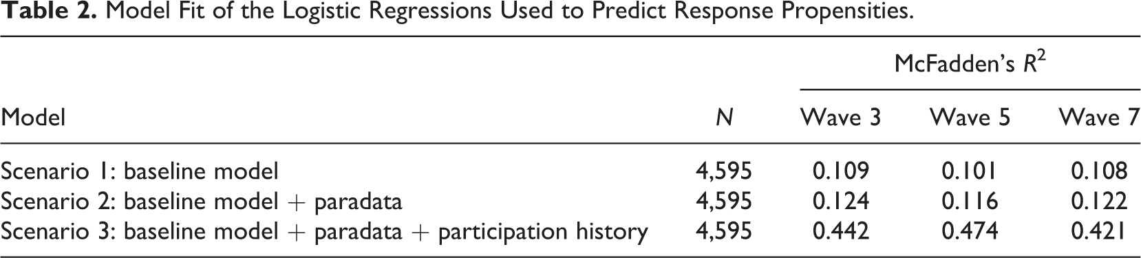
Our results show that including paradata in Scenarios 2 and 3 increased the model fit and, thus, the prediction of panel attrition compared to the baseline Scenario 1. However, the increase in McFadden’s R² for Scenario 3 was remarkably higher compared to the improvement from Scenario 1 to Scenario 2. The second scenario extended the baseline model with a selection of ready-to-use paradata variables. Obviously, these variables had a significant but limited effect on the predictive quality of the panel attrition model. A further extension of the model with a measure of the respondents’ participation history in the online access panel in Scenario 3 strongly boosted the model fit. We observed this pattern for each of the three transitions, which we considered to be an indication of the robustness of our findings.

To get a more detailed picture of the effect of including paradata in the panel attrition models, we re-ran the models, adding each paradata variable separately to Scenario 1 (Table 3). The results can be interpreted as the outcome if Scenario 1 had been only extended with the respective variable.

Table 3.

Statistics on the Paradata Variables Included in the Response Propensity Models.

Variable	AME			Δ(R²)	Δ(AIC)	LR test
Variable	Separate Models	Scenario 2	Scenario 3	Δ(R²)	Δ(AIC)	LR test
Wave 3
No. of control questions correctly answered	0.016	0.023*	0.011	0.001	−1.07	3.08
No. of INR	−0.004***	−0.004**	−0.001	0.003	−8.47	10.47**
No. of DK responses	0.001	0.001	0.001	0.000	0.81	1.19
Smartphone	−0.082***	−0.039	−0.015	0.003	−7.19	11.19**
Tablet	0.002	0.013	0.045
Response speed index	−0.135***	−0.136***	−0.002	0.009	−30.79	32.79***
Participation in 2009	−0.022	−0.034**	0.027**	0.001	−0.69	2.69
No. of completed surveys in last 3 months	0.024***	–	0.023***	0.329	−1262.48	1264.48***
Wave 5
No. of control questions correctly answered	0.008	0.017	0.001	0.000	1.38	0.62
No. of INR	−0.005***	−0.005***	−0.001	0.003	−11.12	13.12***
No. of DK responses	0.002	0.002	0.003**	0.001	−0.35	2.35
Smartphone	−0.061*	−0.006	0.024	0.001	−0.87	4.87
Tablet	0.012	0.025	0.057*
Response speed index	−0.172***	−0.178***	−0.019	0.011	−43.50	45.50***
Participation in 2009	−0.017	−0.033*	0.040***	0.000	0.67	1.33
No. of completed surveys in last 3 months	0.027***	–	0.028***	0.366	−1572.47	1574.47***
Wave 7
No. of control questions correctly answered	0.025**	0.033***	0.020*	0.002	−4.82	6.82**
No. of INR	−0.005***	−0.005***	−0.001	0.003	−11.89	13.89***
No. of DK responses	0.001	0.001	0.001	0.000	1.46	0.54
Smartphone	−0.052	−0.002	0.032	0.001	−0.24	4.24
Tablet	−0.033	−0.019	0.008
Response speed index	−0.151***	−0.156***	−0.001	0.008	−32.66	34.66***
Participation in 2009	0.010	−0.005	0.064***	0.000	1.53	0.47
No. of completed surveys in last 3 months	0.025***	–	0.026***	0.301	−1313.06	1315.06***

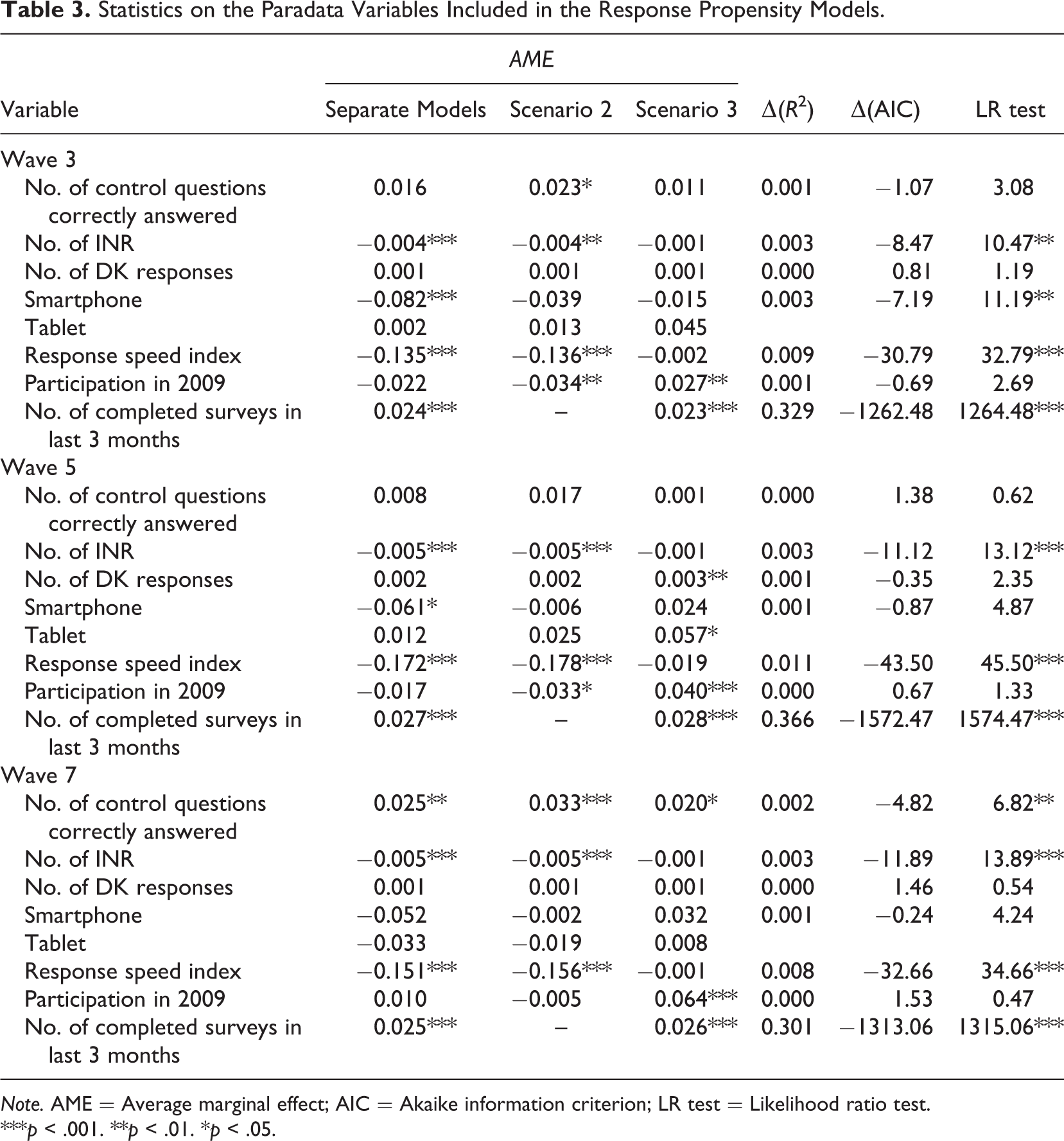
Note. AME = Average marginal effect; AIC = Akaike information criterion; LR test = Likelihood ratio test.

***p < .001. **p < .01. *p < .05.

The second column contains the average marginal effects (AMEs) of the paradata variables, whereas the Columns 3 and 4 show the AMEs of the respective variables when controlling for the other variables included in Scenarios 2 and 3. To assess the change in model fit, we calculated the increase in the Mc Fadden’s R² statistics, Δ(R²), and the increase in the Akaike Information Criterion (AIC), Δ(AIC). Finally, we ran the likelihood ratio tests to verify whether an increase in model fit was significant (Columns 5–7 in Table 3).

Although we found significantly improved predictions of panel attrition for the majority of the tested variables, some variables failed to help us understand and explain this form of nonresponse. The number of item nonresponses, the response speed index, and the respondents’ participation history were the most influential predictors in regard to the improvement in model fit over all three transitions. The results were less clear for the usage of tablets and smartphones, the number of correctly answered control questions, the number of “don’t know” answers, and participation in the 2009 panel survey. We found significant effects for these variables in some of the models, but not in others. Thus, the effects of these variables did not seem to be robust to variations in context. Hence, we focused on the variables for which we found stable effects. To gain deeper insights into their effects on panel attrition, we plotted the predicted probabilities of participation in consecutive panel waves for the number of item nonresponses (Figure 2), the response speed index (Figure 3), and the respondents’ participation history in the online access panel (Figure 4). The most important finding was that the effect of the participation history was very strong and centered on the first quarter of the variable’s range. If a panelist completed more than 10 surveys within the preceding 3 months, participation in subsequent waves of the panel was very likely. Beyond this threshold, it became less important how many more surveys a respondent completed. The effects of item nonresponse and average response speed were rather different. Item nonresponse exerted a strong effect on the average predicted probabilities of continued participation—dropping from approximately 0.8 for respondents with no item nonresponse to 0.1 for respondents with very high numbers of item nonresponses. The effect of the average response speed was considerably lower by comparison. The average predicted probabilities decreased from approximately 0.9 for very fast answering respondents to 0.6 for very slow respondents. To conclude, we found that the respondents’ participation history in the online access panel strongly increased the predictive power of the panel attrition models, whereas other paradata variables improved our models to a lesser extent. Still, some of the paradata variables did not contribute to the understanding and explanation of panel attrition at all. Apart from that, our results clearly show that some paradata variables have the potential of increasing the predictive power of panel attrition models.

Figure 2.

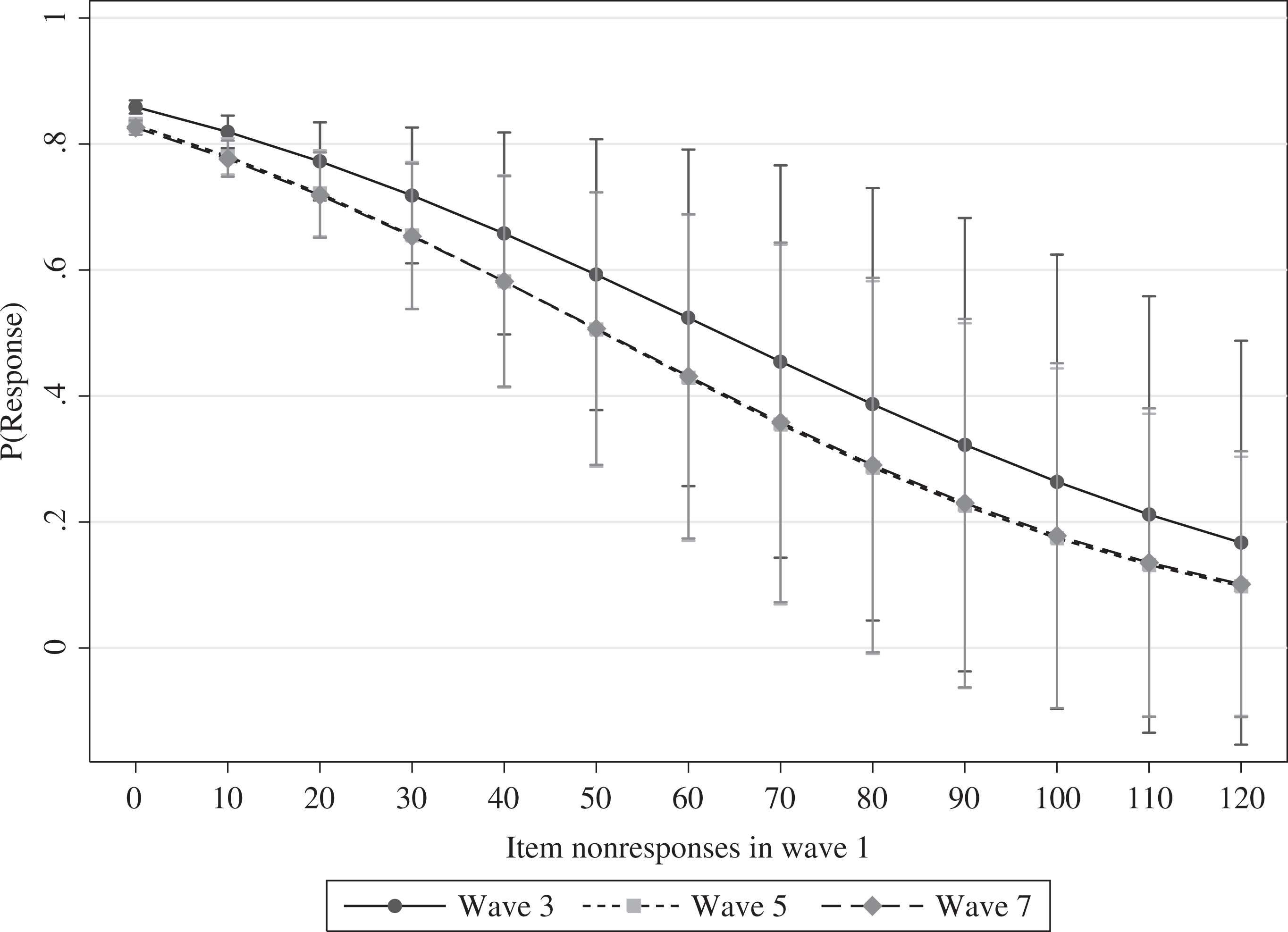
Predictive margins of item nonresponse in Wave 1 on the probability of response to the panel survey Waves 3, 5, and 7.

Figure 3.

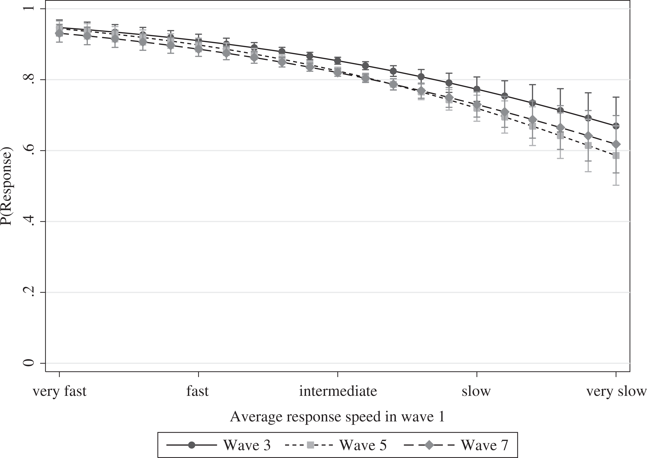
Predictive margins of the response speed index in Wave 1 on the probability of response to the panel survey Waves 3, 5, and 7.

Figure 4.

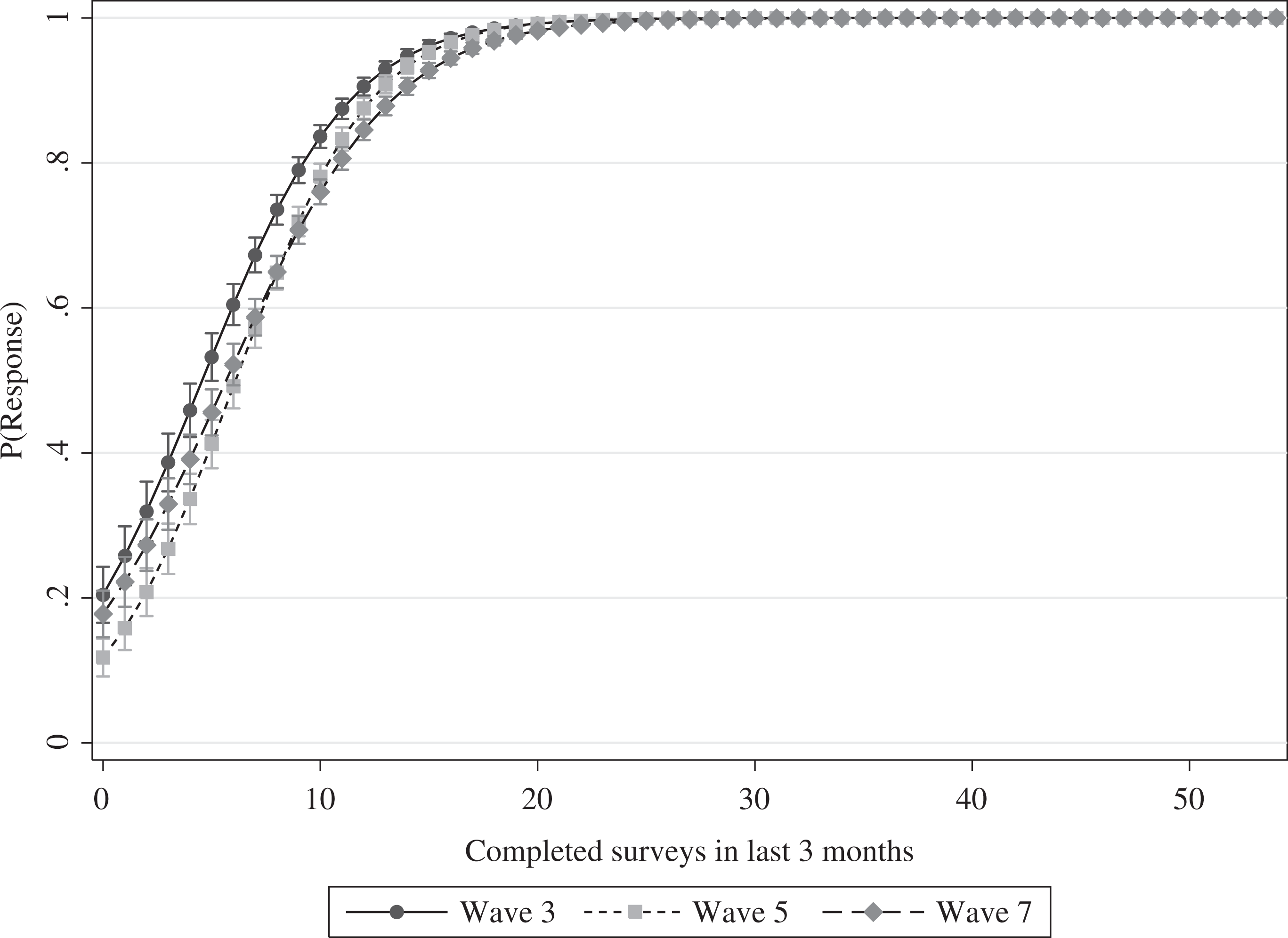
Predictive margins of the number of completed surveys in the last 3 months on the probability of response to the panel survey Waves 3, 5, and 7.

Do Propensity Score Weights Reduce Bias?

As we have seen so far, using a set of paradata variables increased model fit and improved the explanation of panel attrition. Still, the question remains whether these benefits help us to reduce the nonresponse bias when applying propensity score weights to our data.

Table 4 presents descriptive statistics on the propensity score weights for each scenario for the transitions from Wave 1 to Waves 3, 5, and 7. A large variation in weighting factors may inflate the variance of the estimators (Kalton & Flores-Cervantes, 2003; Kish, 1990), whereas extreme weighting factors will make some data points very influential, potentially resulting in outliers (e.g., Liu, Ferraro, Wilson, & Brick, 2004). We found that the variance and the maximum values of the weighting factors increased with the number of paradata variables that we added to the panel attrition models. In other words, we predicted a higher amount of low response propensities, which convert into high weighting factors. This result was especially the case when we added the respondents’ participation history to the attrition model, which led to the estimation of more extreme predicted probabilities.

Table 4.

Summary Statistics on the Propensity Score Weights.

	N	M	SD	Min	Max
Wave 3
Scenario 1: baseline model	4,432	1.00	0.16	0.86	3.98
Scenario 2: baseline model + paradata	4,432	1.00	0.20	0.85	5.99
Scenario 3: baseline model + paradata + participation history	4,432	1.00	0.46	0.87	15.34
Wave 5
Scenario 1: baseline model	4,257	1.00	0.17	0.83	3.30
Scenario 2: baseline model + paradata	4,257	1.00	0.21	0.83	4.65
Scenario 3: baseline model + paradata + participation history	4,257	1.00	0.61	0.85	22.83
Wave 7
Scenario 1: baseline model	4,231	1.00	0.19	0.83	4.40
Scenario 2: baseline model + paradata	4,231	1.00	0.23	0.82	4.92
Scenario 3: baseline model + paradata + participation history	4,231	1.00	0.51	0.84	15.83

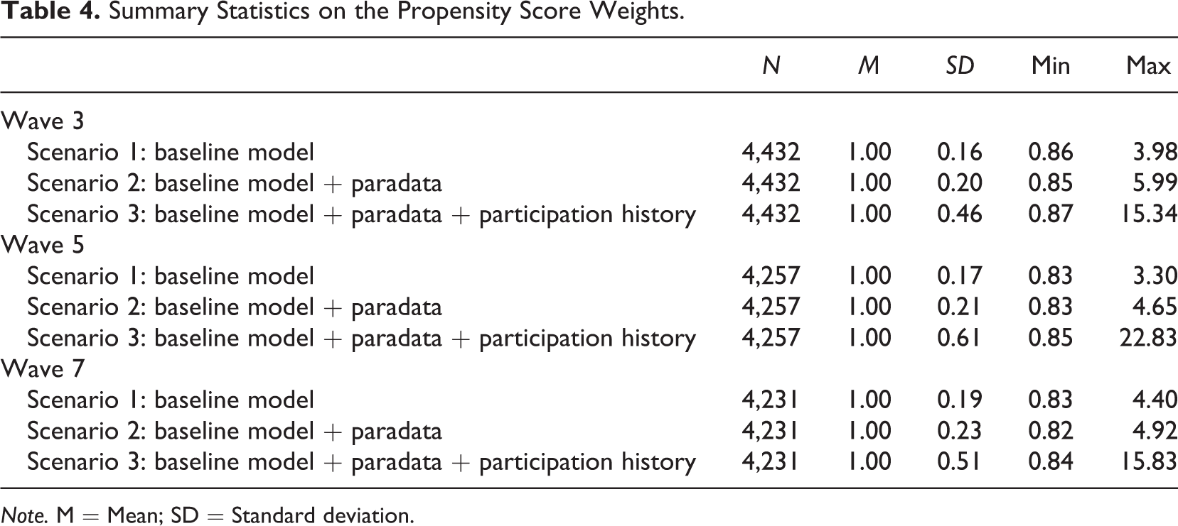
Note. M = Mean; SD = Standard deviation.

To study the capability of paradata to improve the outcome of using propensity score weights, we compared the magnitude of the bias in variables of interest before and after weighting the data as outlined in the “Method” section of this article (Table 5).

Table 5.

Statistics on Dissimilarity Indices.

		Unweighted	Weighted
		Unweighted	Scenario 1	Scenario 2	Scenario 3
Average bias in percentage points	Wave 3	5.90	5.48	5.46	5.59
	Wave 5	6.03	5.56	5.55	5.71
	Wave 7	7.06	6.71	6.67	6.73
Average absolute change in bias	Wave 3		−0.42	−0.44	−0.31
	Wave 5		−0.47	−0.47	−0.32
	Wave 7		−0.34	−0.39	−0.33
Percentage of items with reduction in bias	Wave 3		84.7	84.7	78.0
	Wave 5		74.6	74.6	69.5
	Wave 7		66.1	66.1	69.5

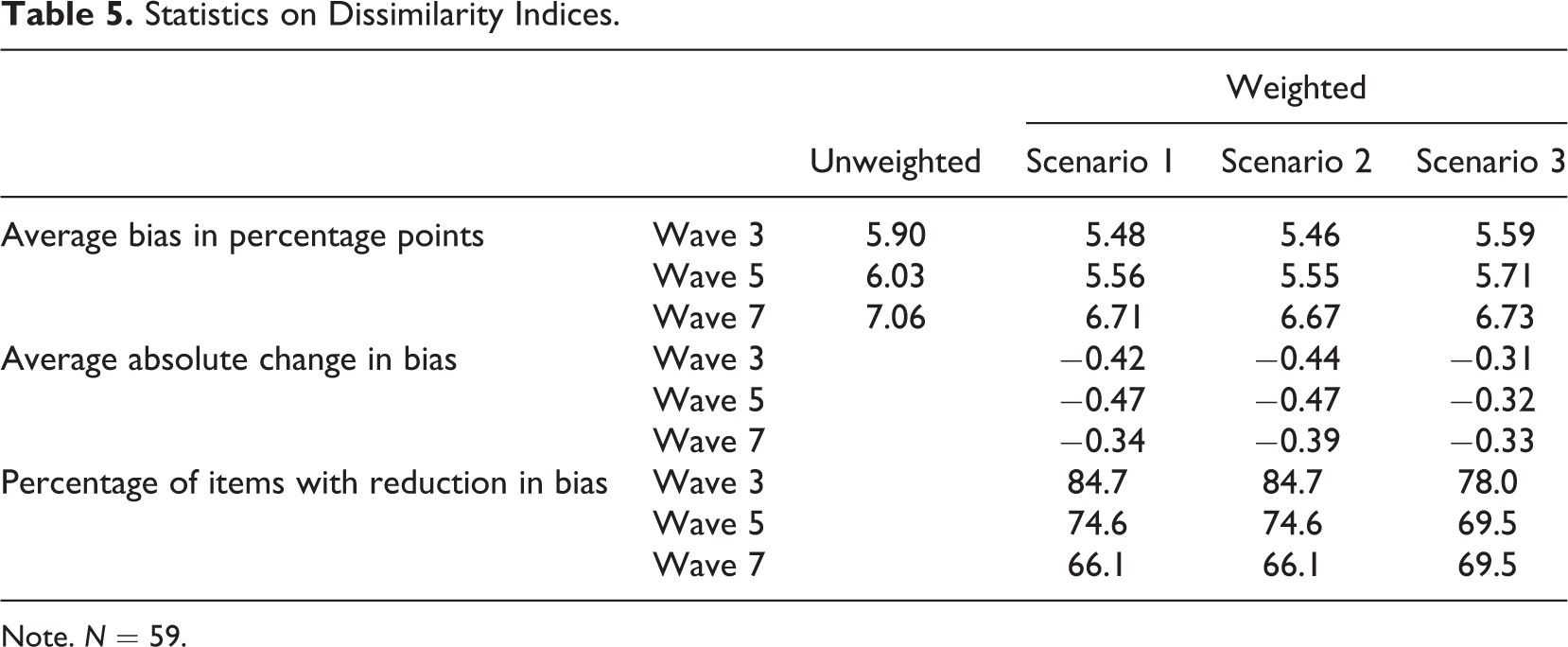
Note. N = 59.

First, looking at the unweighted values of our measure of bias, we found that the average bias increased from 5.90 percentage points in Wave 3 to 7.06 percentage points in Wave 7. This finding can be explained by the increasing number of permanent nonparticipants in the panel. Under the assumption that panel attrition is caused by systematic patterns, a rising cumulative number of nonparticipants results in increasing bias.⁴

The second set of results sheds light on the effectiveness of propensity score weighting. The figures on the average bias in percentage points show that applying the weights to the data reduced the bias. Still, weighting did not eliminate the bias completely in any of the three scenarios. A major fraction of the bias remained uncorrected. The absolute average change of a bias varied between −0.31 and −0.47 percentage points, depending on the wave and scenario. The rather low decrease in the average bias after weighting also can be attributed to the fact that weighting actually increased bias in some variables. Kernel density plots of the distribution of the absolute change in bias across the 59 items illustrate this finding in more detail (Figure 5). They show a reduction in bias for 66.1–84.7% of the variables. This means that the bias increased in 25.3–33.9% of the variables. Still, weighting decreased the bias for a majority of the variables. Furthermore, the rate of successful weighting decreased from Waves 3 to 7. Figure 5 illustrates that the density on the right side of the zero axes increased from Waves 3 through 7. In addition, the density functions flattened, which means that more items experienced a stronger decrease or increase in bias in Waves 5 and 7 compared to Wave 3. We expect these findings to be a result of cumulated unexplained attrition over time, which first increased the average bias and, second decreased the rate of successful weighting.

Figure 5.

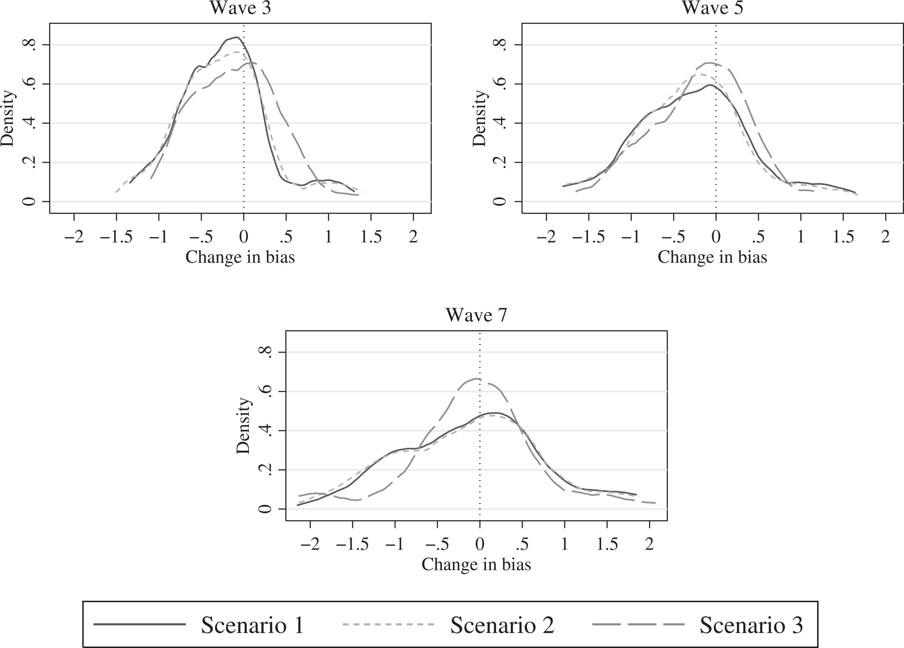
Change in panel attrition bias after weighting.

A third set of results showed that propensity score weighting using paradata (Scenario 2) yielded the largest reduction of bias on average followed by the baseline model (Scenario 1). In addition, Figure 5 shows that marginally more items experienced a stronger reduction in bias, whereas slightly fewer items experienced a stronger increase in bias under Scenario 2 compared to Scenario 1, especially in Waves 3 and 7. However, the rate of successfully weighted items was approximately the same for both scenarios. Adding the respondents’ participation history (Scenario 3) to the attrition model led to the calculation of weights, which corrected for biases to a lesser extent and for fewer variables (with the notable exception of Wave 7). These findings support the argument by Kreuter and Olson (2011) that the variables used in the logistic regressions should be correlated with the attrition process as well as with the variables of interest. Scenario 3 was characterized by the inclusion of a very strong predictor that contributed to model fit but not to the theoretical explanation of the link between attrition and the variables of interest. In this regard, we interpret our findings as a warning to the proponents of a “mechanical” approach that aims at boosting the fit of the attrition model without sound consideration of the theoretical link between the survey response process and the variables of interest.⁵

Discussion

In recent years, increasingly, paradata have been used to analyze respondents’ response behaviors. This trend is particularly true for web surveys. Due to its technical advantages, this data collection mode enables us to collect a large variety of paradata in a cost-efficient way. However, up to now, little is known about whether these data can help us to correct nonresponse biases in surveys.

A frequently used approach to deal with panel attrition is to provide data users with propensity score weights. Similar to other methods, propensity score weighting relies on modeling the process of nonresponse (for a comparision of multiple imputation and propensity score weighting, see Alanya, Wolf, & Soto, 2015). In the light of increasing popularity and availability of paradata, we raised two important questions: First, can a set of widely available paradata help us to improve models of the attrition process? Second, can these paradata help us to create more effective propensity score weights?

First, our results showed that using a set of paradata improved models of panel attrition in a panel survey. However, only some of the paradata variables contributed significantly to the prediction of panel attrition, whereas others did not. Notably the respondents’ participation history proved to be a very strong predictor of participation in consecutive waves of the panel surveys. Including this variable strongly boosted the fit of the attrition model. Other paradata variables, such as the number of item nonresponses or the response speed index, also significantly improved the prediction model. However, including them enhanced the model fit only modestly. These findings show that including these specific paradata variables do not supersede the use of sociodemographic, personality, survey evaluation, and attitudinal variables; rather, these specific variables complement the theoretically grounded panel attrition models. Therefore, the present study provides researchers with evidence on several auxiliary variables that may be considered when designing a panel survey (and more so for a web-based panel survey).

Second, our results on the effectiveness of propensity score weights in reducing attrition biases highlighted the applicability of paradata. However, our findings stressed the need to fit explanatory models with variables that correlate well with the attrition process and the variables of interest. In this respect, our results—which are based on real data—are in line with the findings of Kreuter and Olson’s (2011) simulation studies. The implication of our research is that it is important to not simply boost model fit but to carefully select the variables for the attrition model. That said, we strongly recommend selecting auxiliary variables on the basis of a theoretically grounded model of the attrition process. As a consequence, it is an important challenge for survey methodology to identify variables that are related to the attrition process and the variables of interest. In practical terms, this means that we have to test whether the propensity score weights do what they are intended to do—reduce panel attrition biases. The present study provides a first contribution to this challenge.

Finally, this study has five limitations that should be addressed in further research. First, we confronted the well-known problem of disentangling panel attrition and panel conditioning when assessing the nonresponse bias. However, we believe this to be a minor issue due to the sampling source. The web-based panel survey uses a sample drawn from an online access panel. Thus, we confidently assumed that the participants are somewhat experienced with web surveys and their commonly used instruments. While evidence on the settings under which panel conditioning occurs is mixed (e.g., Warren & Halpern-Manners, 2012), learning effects are likely a part of the explanation. For instance, respondents learn how to answer common types of survey questions and how they can reduce the response burden by changing their answering behavior. As learning curves are usually asymptotical, the effect of panel conditioning should be much smaller for participants of an online access panel compared to a sample of inexperienced respondents.

Second, our findings are based on analyses of data from web-based surveys. As has been shown, web surveys provide ample opportunities to collect paradata. However, future research should extend this line of research to other data collection modes (e.g., telephone or face-to-face interviewing) and collect evidence on a similar set of paradata. Yet, we believe our general findings apply to different modes as well. In this respect, more attention should be directed to understanding the magnitude of how paradata contribute to predicting and correcting for attrition biases. Moreover, a critical review of how easily useful paradata can be obtained in different modes may prove helpful.

Third, we evaluated the performance of one specific class of propensity score weights under three scenarios with regard to the reduction in nonresponse bias in the variables of interest. To a certain extent, this approach limits the generalizability of our findings. On the one hand, other methods exist that rely on propensity scores to generate weights, for example, the method of creating propensity strata. On the other hand, propensity score weights are sometimes suspected to inflate standard errors of estimates. Thus, we strongly encourage further research to broaden the scope of our findings by considering additional methods and indicators.

Fourth, a major advantage of our study is that we were able to quantify nonresponse bias for a large number of substantive variables. Yet, the vast quantity of variables made it necessary to rely on averaged indicators, thus, potentially losing additional insights. This design decision inevitably involved a trade-off between the generality and specificity of the findings. Thus, we encourage further work to closely inspect the nonresponse bias for subsets of variables.

Finally, we analyzed data from a panel survey on political attitudes and behavior. Although we believe that it is unlikely that our results depend on the topic of the survey, we cannot completely preclude this possibility. Thus, we stress the value of replications of our analyses using data from panel surveys with different topics.

In conclusion, we identified a set of easily available and applicable paradata that provided a better understanding and modeling of the attrition process in panel surveys. Moreover, some of these paradata were also suited to improving propensity score weights, which aimed at the reduction of panel attrition biases. However, as our analyses show, using this set of paradata to compute propensity score weights was not a panacea to panel attrition biases. Further research is still necessary on the theoretical explanation of the attrition process and methods to correct for panel attrition biases. The further development of a tool kit of easily available and applicable auxiliary variables for use with nonresponse bias correction methods would be of enormous value to survey methodology.

Footnotes

Appendix A

Table A1.

Variables Used to Evaluate Attrition Bias in Consecutive Panel Waves

Variable	Label	Scale	Coding
1	Interest in politics	Ordinal	1-5
2	Voting intention/Actual voting behavior: first vote	Categorial	1-801
3	Voting intention/Actual voting behavior: second vote	Categorial	1-801
4	Scalometer parties: CDU	Ordinal	1-11
5	Scalometer parties: CSU	Ordinal	1-11
6	Scalometer parties: SPD	Ordinal	1-11
7	Scalometer parties: FDP	Ordinal	1-11
8	Scalometer parties: GRÜNE	Ordinal	1-11
9	Scalometer parties: DIE LINKE	Ordinal	1-11
10	Scalometer parties: PIRATEN	Ordinal	1-11
11	Scalometer parties: AfD	Ordinal	1-11
12	Scalometer government	Ordinal	1-11
13	Scalometer politicians: Angela Merkel	Ordinal	1-11
14	Scalometer politicians: Peer Steinbrück	Ordinal	1-11
15	Scalometer politicians: Horst Seehofer	Ordinal	1-11
16	Scalometer politicians: Rainer Brüderle	Ordinal	1-11
17	Scalometer politicians: Jürgen Trittin	Ordinal	1-11
18	Scalometer politicians: Gregor Gysi	Ordinal	1-11
19	Ability to solve the most important issue	Categorial	1-809
20	Ability to solve the second most important issue	Categorial	1-809
21	Preferred chancellor	Categorial	1-3
22	Socio-economic dimension, ego	Ordinal	1-7
23	Left-right-authoritarian, ego	Ordinal	1-7
24	Climate protection, ego	Ordinal	1-7
25	Importance fairness of income	Ordinal	1-5
26	Fairness of income, parties: CDU/CSU	Ordinal	1-5
27	Fairness of income, parties: SPD	Ordinal	1-5
28	Fairness of income, parties: FDP	Ordinal	1-5
29	Fairness of income, parties: GRÜNE	Ordinal	1-5
30	Fairness of income, parties: DIE LINKE	Ordinal	1-5
31	Left–right assessment, parties: CDU	Ordinal	1-11
32	Left–right assessment, parties: CSU	Ordinal	1-11
33	Left–right assessment, parties: SPD	Ordinal	1-11
34	Left–right assessment, parties: FDP	Ordinal	1-11
35	Left–right assessment, parties: GRÜNE	Ordinal	1-11
36	Left–right assessment, parties: DIE LINKE	Ordinal	1-11
37	Left–right assessment, parties: PIRATEN	Ordinal	1-11
38	Left–right assessment, parties: AfD	Ordinal	1-11
39	Left–right self assessment	Ordinal	1-11
40	Attention to election campaign	Ordinal	1-5
41	European aid, chancellor candidates: Angela Merkel	Ordinal	1-7
42	European aid, chancellor candidates: Peer Steinbrück	Ordinal	1-7
43	European aid, ego	Ordinal	1-7
44	Performance chancellor candidates, European financial crisis: Angela Merkel	Ordinal	1-5
45	Performance chancellor candidates, European financial crisis: Peer Steinbrück	Ordinal	1-5
46	Conversations about politics, current: friends	Ordinal	1-8
47	Conversations about politics, current: partner/spouse	Ordinal	1-8
48	Conversations about politics, current: relatives	Ordinal	1-8
49	Conversations about politics, current: colleagues/friends from college	Ordinal	1-8
50	Conversations about politics, current: acquaintances, neighbors	Ordinal	1-8
51	Conversations about politics, current: I didn’t talk about politics	Categorial	1-2
52	Discussion partner 1, voting decision	Categorial	1-801
53	Opinions about the NSA scandal: merkel reacted appropriately	Ordinal	1-5
54	Opinions about the NSA scandal: federal government was informed	Ordinal	1-5
55	Opinions about the NSA scandal: parties in opposition were informed	Ordinal	1-5
56	Party identification	Categorial	2-808
57	Party identification, strength	Ordinal	1-5
58	Attention survey participation	Ordinal	1-5
59	Rating of survey	Ordinal	1-5

Declaration of Conflicting Interests

The authors declared no potential conflicts of interest with respect to the research, authorship, and/or publication of this article.

Funding

The authors received no financial support for the research, authorship, and/or publication of this article.

Notes

References

Alanya

Wolf

Soto

(2015). Comparison of multiple imputation and propensity score weighting in unit nonresponse adjustments: A simulation study. Public Opinion Quarterly. doi:dx.doi.org/10.1093/poq/nfv029

Andreß

H. -J.

Golsch

Schmidt

A. W.

(2013). Applied panel data analysis for economic and social surveys. Heidelberg, New York, Dordrecht, London: Springer.

Bassili

J. N.

(1993). Response latency versus certainty as indexes of the strength of voting intentions in a CATI survey. Public Opinion Quarterly, 57, 54–61.

Bassili

J. N.

Scott

B. S.

(1996). Response latency as a signal to question problems in survey research. Public Opinion Quarterly, 60, 390–399.

Beatty

Herrmann

(2002). To answer or not to answer: Decision processes related to survey item nonresponse. In Groves

R. M.

Dillman

D. A.

Eltinge

J. L.

Little

R. J. A.

(Eds.), Survey nonresponse (pp. 71–85). New York, NY: Wiley.

Bergmann

(2011). Propensity score weighting: Methods and applications. Paper presented at the 4th Conference of the European Survey Research Association (ESRA), Lausanne, Switzerland.

Bethlehem

(2002). Weighting nonresponse adjustments based on auxiliary information. In Groves

R. M.

Dillman

D. A.

Eltinge

J. L.

Little

R. J. A.

(Eds.), Survey nonresponse (pp. 275–288). New York, NY: Wiley.

Biemer

P. P.

Chen

Wang

(2013). Using level-of-effort paradata in non-response adjustments with application to field surveys. Journal of the Royal Statistical Society: Series A (Statistics in Society), 176, 147–168. doi:10.1111/j.1467-985X.2012.01058.x

Blumenstiel

J. E.

Gummer

(2015). Prävention, Korrektur oder beides? Drei Wege zur Reduzierung von Nonresponse Bias mit Propensity Scores. In Schupp

Wolf

(Eds.), Nonresponse bias: Qualitätssicherung sozialwissenschaftlicher umfragen (pp. 11–42). Wiesbaden, Germany: VS Verlag.

10.

Callegaro

(2013). Paradata in web surveys. In Kreuter

(Ed.), Improving surveys with paradata: Analytic uses of process information (pp. 261–280). Hoboken, NJ: Wiley.

11.

Callegaro

Yang

Bhola

D. S.

Dillman

D. A.

Chin

T. -Y.

(2009). Response latency as an indicator of optimizing in online questionnaires. Bulletin de Méthodologie Sociologique, 103, 5–25. doi:10.1177/075910630910300103

12.

Couper

M. P.

(2000). Usability evaluation of computer-assisted survey instruments. Social Science Computer Review, 18, 384–396. doi:10.1177/089443930001800402

13.

Couper

M. P.

Kreuter

(2013). Using paradata to explore item level response times in surveys. Journal of the Royal Statistical Society: Series A (Statistics in Society), 176, 271–286. doi:10.1111/j.1467-985X.2012.01041.x

14.

De Bruijne

Wijnant

(2013). Comparing survey results obtained via mobile devices and computers: An experiment with a mobile web survey on a heterogeneous group of mobile devices versus a computer-assisted web survey. Social Science Computer Review, 31, 482–504. doi:10.1177/0894439313483976

15.

Duncan

G. J.

Kalton

(1987). Issues of design and analysis of surveys across time. International Statistical Review, 55, 97–117.

16.

Duncan

O. D.

Duncan

(1955). A methodological analysis of segregation indexes. American Sociological Review, 20, 210–217.

17.

Fazio

R. H.

(1990). Multiple processes by which attitudes guide behavior: The MODE model as an integrative framework. In Zanna

M. P.

(Ed.), Advances in experimental social psychology (Vol. 23, pp. 75–109). San Deigo, CA: Academic Press.

18.

Fazio

R. H.

Sanbonmatsu

D. M.

Powell

M. C.

Kardes

F. R.

(1986). On the automatic activation of attitudes. Journal of Personality and Social Psychology, 50, 229–238.

19.

Festinger

(1957). A theory of cognitive dissonance. Stanford, CA: Stanford University Press.

20.

Firebaugh

(2008). Seven rules for social research. Princeton, NJ: Princeton University Press.

21.

Fricker

Tourangeau

(2010). Examining the relationship between nonresponse propensity and data quality in two national household surveys. Public Opinion Quarterly, 74, 934–955. doi:10.1093/poq/nfq064

22.

Greszki

Meyer

Schoen

(2014). The impact of speeding on data quality in nonprobability and freshly recruited probability-based online panels. In Callegaro

Baker

Bethlehem

Göritz

A. S.

Krosnick

J. A.

Lavrakas

P. J.

(Eds.), Online panel research: A data quality perspective (pp. 238–262). Chichester, England: Wiley.

23.

Groves

R. M.

(2006). Nonresponse rates and nonresponse bias in household surveys. Public Opinion Quarterly, 70, 646–675.

24.

Groves

R. M.

Fowlers

F. J.

Couper

M. P.

Lepkowski

J. M.

Singer

Tourangeau

(2009). Survey methodology. Hoboken, NJ: John Wiley & Sons.

25.

Gummer

Roßmann

(2015). Explaining interview duration in web surveys: A multilevel approach. Social Science Computer Review, 33, 217–234. doi:10.1177/0894439314533479

26.

Halaby

C. N.

(2004). Panel models in sociological research: Theory into practice. Annual Review of Sociology, 30, 507–544. doi:10.1146/annurev.soc.30.012703.110629

27.

Heerwegh

(2003). Explaining response latencies and changing answers using client-side paradata from a web survey. Social Science Computer Review, 21, 360–373. doi:10.1177/0894439303253985

28.

Horvitz

D. G.

Thompson

D. J.

(1952). A generalization of sampling without replacement from a finite universe. Journal of the American Statistical Association, 47, 663–685.

29.

Link

M. W.

Murphy

Schober

M. F.

Buskirk

T. D.

Hunter Childs

Langer Tesfaye

(2014). Mobile technologies for conducting, augmenting and potentially replacing surveys: Executive summary of the AAPOR Task Force on Emerging Technologies in Public Opinion Research. Public Opinion Quarterly, 78, 779–787. doi:10.1093/poq/nfu054

30.

Kaczmirek

(2008). Human-survey interaction. Usability and nonresponse in online surveys. Mannheim, DE: University of Mannheim.

31.

Kalton

Flores-Cervantes

(2003). Weighting methods. Journal of Official Statistics, 19, 81–97.

32.

Kish

(1990). Weighting: Why, when, and how? Proceedings of the survey research methods section of the American Statistical Association, USA, 121–130.

33.

Kreuter

Couper

M. P.

Lyberg

L. E.

(2010). The use of paradata to monitor and manage survey data collection. Paper presented at the Joint Statistical Meetings of the American Statistical Association July 31–August 5, 2010, Vancouver, Canada.

34.

Kreuter

Olson

(2011). Multiple auxiliary variables in nonresponse adjustment. Sociological Methods & Research, 40, 311–332. doi:10.1177/0049124111400042

35.

Kreuter

Olson

(2013). Paradata for nonresponse error investigation. In Kreuter

(Ed.), Improving surveys with paradata: Analytic uses of process information (pp. 13–42). Hoboken, NJ: Wiley.

36.

Kroh

Spieß

(2008). Documentation of sample sizes and panel attrition in the German Socio Economic Panel (SOEP) (1984 until 2007). Data documentation, 39. Berlin, DE: DIW.

37.

Krosnick

J. A.

(1991). Response strategies for coping with the cognitive demands of attitude measures in surveys. Applied Cognitive Psychology, 5, 213–236. doi:10.1002/acp.2350050305

38.

Krosnick

J. A.

(1999). Survey research. Annual Review of Psychology, 50, 537–567.

39.

Lepkowski

J. M.

Couper

M. P.

(2002). Nonresponse in the second wave of longitudinal household surveys. In Groves

R. M.

Dillman

D. A.

Eltinge

J. L.

Little

R. J. A.

(Eds.), Survey nonresponse (pp. 259–272). New York, NY: John Wiley & Sons.

40.

Little

R. J. A.

Vartivarian

(2005). Does weighting for nonresponse increase the variance of survey means? Survey Methodology, 31, 161–168.

41.

Liu

Ferraro

Wilson

Brick

M. J.

(2004). Trimming extreme weights in household surveys. Proceedings of the survey research methods section of the American Statistical Association, USA, 3905–3912.

42.

Lynn

(2009). Methods for longitudinal suveys. In Lynn

(Ed.), Methodology of longitudinal suveys (pp. 1–19). Chichester, England: Wiley.

43.

Malhotra

(2008). Completion time and response order effects in web surveys. Public Opinion Quarterly, 72, 914–934. doi:10.1093/poq/nfn050

44.

Mavletova

(2013). Data quality in PC and mobile web surveys. Social Science Computer Review, 31, 725–743. doi:10.1177/0894439313485201

45.

Olson

Parkhurst

(2013). Collecting paradata for measurement error evaluations. In Kreuter

(Ed.), Improving surveys with paradata (pp. 43–72). Hoboken, NJ: Wiley.

46.

Peytchev

Hill

C. A.

(2010). Experiments in mobile web survey design: Similarities to other modes and unique considerations. Social Science Computer Review, 28, 319–335. doi:10.1177/0894439309353037

47.

Rattinger

Roßteutscher

Schmitt-Beck

Weßels

Wolf

(2014). Short-term campaign panel 2013 (GLES) with supplemental cross-sections. Cologne, DE: GESIS Data Archive. doi:10.4232/1.11846, doi:10.4232/1.11777, doi:10.4232/1.11778, doi:10.4232/1.11779

48.

Rosenbaum

P. R.

Rubin

D. B.

(1983). The central role of the propensity score in observational studies for causal effects. Biometrika, 70, 41–55. doi:10.1093/biomet/70.1.41

49.

Roßmann

(2015). RSPEEDINDEX: Stata module to compute a response speed index and perform outlier identification (Version 0.4) [Computer Software]. Chestnut Hill, MA: Boston College. Retrieved from http://econpapers.repec.org/software/bocbocode/s458007.htm

50.

Roßmann

Blumenstiel

J. E.

Steinbrecher

(2014). Why do respondents break off web surveys and does it matter? Results from four follow-up surveys. International Journal of Public Opinion Research. doi:10.1093/ijpor/edu025

51.

Roßmann

Gummer

(2014). PARSEUAS: Stata module to extract detailed information from user agent strings (Version 1.0) [Computer Software]. Chestnut Hill, MA: Boston College. Retrieved from http://EconPapers.repec.org/RePEc:boc:bocode:s457937

52.

Rubin

D. B.

(1987). Multiple imputation for nonresponse in surveys. New York, NY: Wiley.

53.

Sakshaug

(2013). Using paradata to study response to within-survey requests. In Kreuter

(Ed.), Improving surveys with paradata (pp. 171–190). Hoboken, NJ: Wiley.

54.

Sinibaldi

Trappmann

Kreuter

(2014). Which is the better investment for nonresponse adjustment: Purchasing commercial auxiliary data or collecting interviewer observations? Public Opinion Quarterly, 78, 440–473. doi:10.1093/poq/nfu003

55.

Stern

M. J.

(2008). The use of client-side paradata in analyzing the effects of visual layout on changing responses in web surveys. Field Methods, 20, 377–398. doi:10.1177/1525822X08320421

56.

Stieger

Reips

U. -D.

(2010). What are participants doing while filling in an online questionnaire: A paradata collection tool and an empirical study. Computers in Human Behavior, 26, 1488–1495.

57.

Vandecasteele

Debels

(2007). Attrition in panel data: The effectiveness of weighting. European Sociological Review, 23, 81–97. doi:10.1093/esr/jcl021

58.

Warren

J. R.

Halpern-Manners

(2012). Panel conditioning in longitudinal social science surveys. Sociological Methods & Research, 41, 491–534.

59.

Watson

Wooden

(2009). Identifying factors affecting longitudinal survey response. In Lynn

(Ed.), Methodology of longitudinal surveys (pp. 157–182). Chichester, England: John Wiley & Sons.

60.

Yan

Tourangeau

(2008). Fast times and easy questions: The effects of age, experience and question complexity on web survey response times. Applied Cognitive Psychology, 22, 51–68.

61.

Zhang

Conrad

F. G.

(2014). Speeding in web surveys: The tendency to answer very fast and its association with straightlining. Survey Research Methods, 8, 127–135.

Using Paradata to Predict and Correct for Panel Attrition

Abstract

Keywords

Introduction

Data

Method

Results

Prediction of Panel Attrition

Do Propensity Score Weights Reduce Bias?

Discussion

Footnotes

Appendix A

Declaration of Conflicting Interests

Funding

Notes

References