Sage Journals: Discover world-class research

Abstract

Overmolding discontinuous fiber-reinforced thermoplastic elements on a continuous fibers base laminate enables to speed up composite manufacturing. The performance of such assemblies depends on numerous factors, whose roles are impossible to isolate and clarify in typical experimental tests on T-joint samples, making it difficult to interpret the experimental results and extrapolate them to other configurations or to obtain design allowables. In this work, the mechanical response of T-joint samples is simulated using of a Cohesive Zone Model (CZM) for the laminate/overmold interface and specific numerical tools to handle instabilities and improve convergence. This virtual testing approach enables us to systematically explore and quantify the effect of bond properties, loading conditions and part geometry on the load bearing capacity of the assembly. Clarifying the failure mechanisms of T-joints and their dependence on the different aspects of the structural problem is paramount for interpreting the results of current T-joint tests in the literature, as well as to design improved testing solutions.

Keywords

Thermoplastic matrix composites overmolding T-joint cohesive zone model virtual testing

Introduction

Continuous fibers, thermoplastic matrix composites have recently gained significant interest with respect to their thermosetting matrix counterparts in application requiring significant load bearing capacities. High performance thermoplastic polymers, in particular of the PEAK family, can be used to manufacture composites with very good thermal and mechanical properties, including a high fracture toughness.¹ Other advantages include the recyclability potential of thermoplastics.²

Due to the high melting temperatures and large viscosity of high performance thermoplastic polymers, the manufacturing processes developed for many decades for thermoset matrix composites cannot be directly applied. On the other hand, the short consolidation times of thermoplastics, together with the increasing automation of manufacturing processes, make this new generation of composites very attractive for applications requiring short cycle times. Overall, manufacturing processes for continuous fibers, thermoplastic matrix composites are currently a very active area of research (see the recent review paper Ref. 2).

Overmolding of structural details, such as ribs, made of discontinuous fiber reinforced thermoplastics onto a continuous fibers composite substrate has emerged as a way to further increase the production speed and obtain net-shape parts. Overmolding, that is injecting a (discontinuous fiber-reinforced) thermoplastic polymer onto a pre-existing substrate, is not a new technique, but its applications have evolved over the years, moving from everyday objects³ to non structural automotive parts⁴ and towards increasingly demanding structural application in the automotive and aeronautic sectors.^5–8 Many papers dealing with this manufacturing process and the resulting properties of the part have been published in the last few years.

During overmolding, the temperature at the contact between the base laminate and the injected material is not uniform,^9–11 leading to specific microstructural features and local properties at and close to the junction:

• Non uniform degrees of crystallinity of the polymer¹² and interpenetration of the molecular chains between the overmold and the base laminate,^10,13–16 leading to a non uniform quality of the bond between these two parts;

• Voids and/or cracks in the overmold^6,17;

• Loss of compaction and/or local deformation of the base laminate, which can partially flow into the rib cavity depending on the substrate temperature during overmolding: in particular, Ref. 18 distinguishes the processes where the base laminate consolidation and overmolding are carried out simultaneously versus sequentially.

All of these features significantly affect the quality, and in particular the mechanical resistance, of the junction between the base laminate and the overmold. For this reason, the load bearing capacity of the assembly is often used as an indicator in studies investigating the influence of different process parameters, such as the temperature of the injected material, the injection and the holding pressures. Since no normalized tests are defined for overmolding, a variety of test setups and loading conditions are considered in the literature: butt joints,⁹ Iosipescu tests,⁹ Single Lap Shear,^15,19–22 different types of peel tests,^20,23 non symmetric Double Cantilever Beam tests.²⁴ The results of these tests are used to extract (average) maximum stresses or fracture energies for different manufacturing parameters. However, local processing conditions can be rather different between different specimen geometries, and a detailed knowledge of the local stress state at the interface is required to extract meaningful material parameters, thus it is not easy to extrapolate the results of these tests to different geometries or loading conditions.

A widespread test for overmolded specimens is a tensile test on a T-joint ministructure, often called “rib pull-off test”, since this specimen geometry is very close to those of real manufactured parts.^{6,8–10,14,18,20,21,25–28} Similar but not identical in-house fixtures are used by different research groups, which involve different solutions to retain the base laminate while a standard uniaxial testing machine grip pulls on the overmold. In addition to manufacturing parameters, the effect of the rib foot shape is often investigated in these studies, and in some cases other aspects are considered, as the width of the specimen²⁸ or fatigue loading conditions.¹⁸ The maximum force or the maximum average stress at the interface are generally extracted from these tests. The strength of the rib is generally a fraction of the strength of the neat polymer material, and it displays a significant variability between samples. There is currently no consensus in the literature on the best practices for T-joint tests, thus results from different works can hardly be compared or extrapolated as they involve significant differences in materials, specimen geometry and boundary conditions.

The problem is that the stress state at the interface during tests on T-joint specimens is not uniform, but it depends in a complex way on the specimen geometry, boundary conditions and local defects. This was recently observed in Ref. 28 by instrumenting T-joint tests with Digital Image Correlation. That experimental paper offers a qualitative discussion of the role of some features of the T-joint test on the overall response, for instance the amount of bending on the base laminate and the rib foot geometry, and it proposes some general recommendations to improve the test method. To the authors’ knowledge, however, no systematic quantitative investigation of the influence of the T-joint test features on its load bearing capacity has been carried out in the literature. This is the subject of the present work.

In this work, virtual testing of T-joint assemblies is carried out using a finite element model, where failure of the bond zone between the base laminate and the overmold is modeled using a Cohesive Zone Model (CZM). Since their beginnings,^29–31 CZM have been extensively used in the literature to simulate delamination between plies in continuous fibers composites or debonding between different types of substrates. A recent paper even used such models to reproduce failure of an overmolded T-joint,27 but, to the authors’ knowledge, no systematic numerical study on this test geometry was carried out before. Therefore, the present work aims to systematically explore and quantify the effects of interface parameters, loading conditions and specimen geometry on the load bearing capacity of the T-joint. In particular, we cover a range of conditions which can be observed in real T-joint tests from the literature: material properties associated to thermoset and thermoplastic composites, different rib foot shapes and base laminate thicknesses, as well as different ways of constraining the base laminate and the effect of a misalignment in the rib tensile load. The results of our simulations show that the load bearing capacity is controlled not only by the strength, but also by the toughness of the interface, depending on the retained geometry and material parameters. Furthermore, we prove the paramount influence of base laminate bending and load misalignment on the load bearing capacity of the T-joint: such aspects depend strongly on the test setup, and they are generally poorly described and possibly not well controlled in most currently published experimental results.

The load bearing capacities predicted by our model are coherent with the experimental ranges obtained in the literature, which constitutes a preliminary validation of the proposed approach. In addition to providing a precious tool to critically interpret existing literature results on T-joint tests, the virtual testing approach proposed here constitutes a key preliminary work to the design of a new experimental setup with improved control of the boundary and loading conditions. This is the subject of a paper in preparation.³²

Material and methods

Modeling aspects

Structural model assumptions

Figure 1 depicts a typical experimental test on a T-joint specimen, from Ref. 8, as well as a schematic of the structural model discussed here. As the aim is to investigate different configurations, different models are build by modifying the features marked in red in Figure 1.

Figure 1.

Typical experimental test on a T-joint, from Ref. 8, (left) and structural model considered in this work (right): dimensions are in millimeters, the features whose influence is explored in this work are marked in red.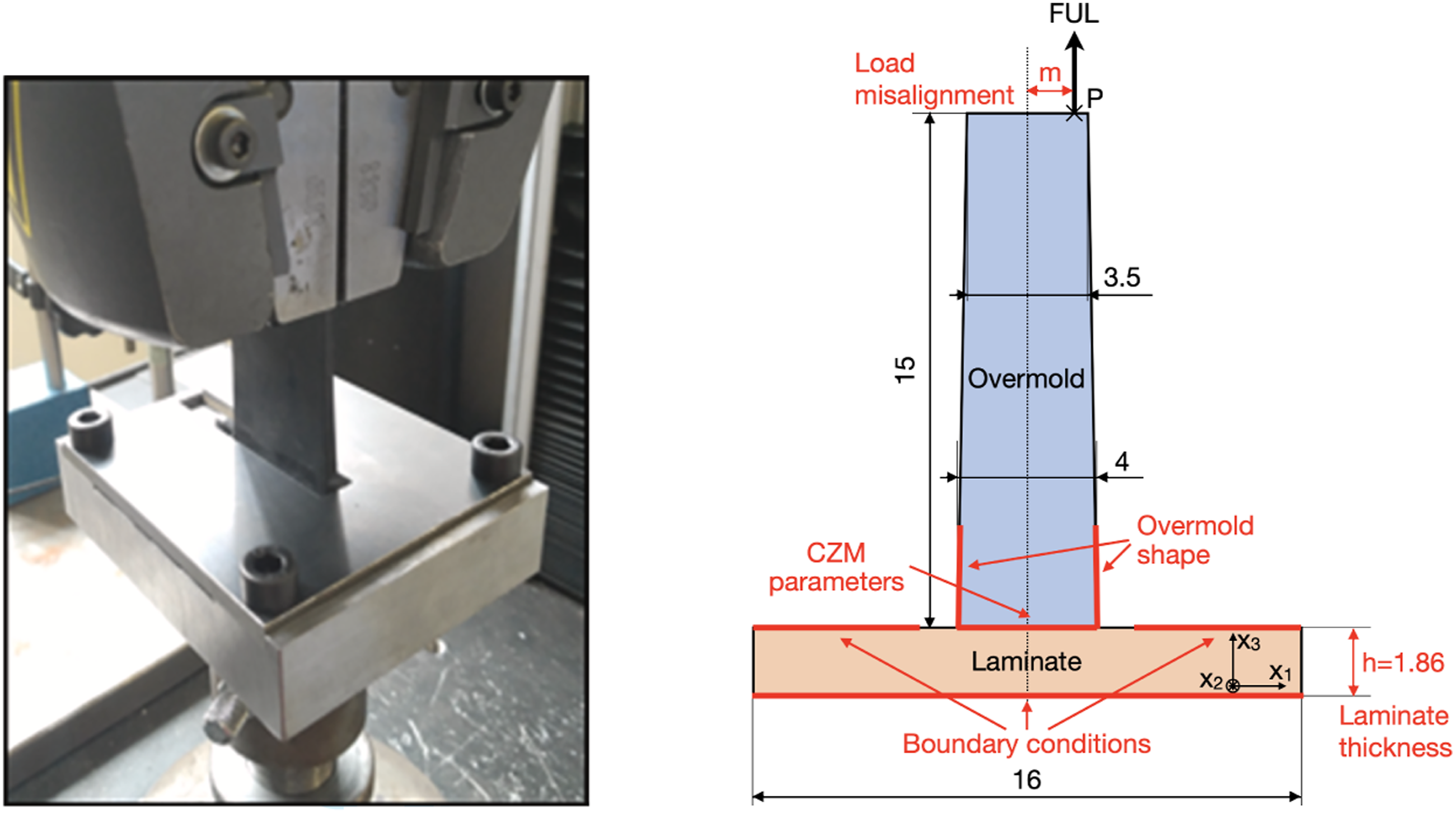

A 2D plane-strain model was chosen, as the fibers in the base laminate restrict deformations out of the (1.3) plane, as well as to reduce the computational cost. The base laminate is restrained with different possible boundary conditions. A uniform vertical displacement is imposed on the top part of the overmold, and a vertical load is applied in correspondence of point P.

Both the base laminate and the overmold are modeled as linear elastic materials, with an orthotropic and an isotropic behavior, respectively. The material parameters reported in Tables 1 and 2 correspond to those of a [0/90] woven carbon/PEKK base laminate and a discontinuous fiber-reinforced carbon/PEKK overmold, manufactured by the Centre Technique des Industries Mécaniques (CETIM), the industrial partner of this work, using the mold represented in Ref. 8. The material parameters are nominal values provided by the material suppliers. Modifying the stiffness of the laminate and/or of the overmold would modify the overall stiffness of the system, as well as the energy stored within it for a given level of applied load. Modifications of the boundary conditions or of the thickness of the base laminate have similar effects, which are investigated in detail later in the paper. The variation of the elastic parameters of the laminate and overmold was not explored here to avoid further increase of the parameter space, but different sets of parameters, corresponding to different laminate and overmold materials, could be considered without loss of generality of the proposed numerical approach.

Table 1.

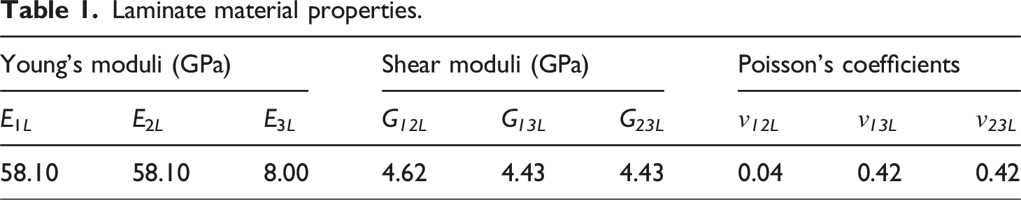
Laminate material properties.

Young’s moduli (GPa)			Shear moduli (GPa)			Poisson’s coefficients
E _1L	E _2L	E _3L	G _12L	G _13L	G _23L	ν _12L	ν _13L	ν _23L
58.10	58.10	8.00	4.62	4.43	4.43	0.04	0.42	0.42

Table 2.

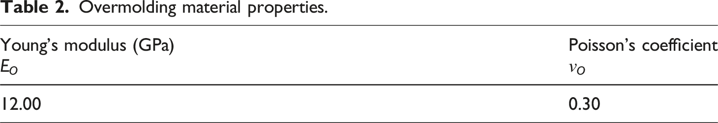
Overmolding material properties.

Young’s modulus (GPa) E_O	Poisson’s coefficient ν_O
12.00	0.30

The progressive failure of the overmold/laminate interface is modeled with a Cohesive Zone Model (CZM).

Cohesive zone models: key aspects

Cohesive Zone Models (CZMs)^29–31 describe the progressive failure of an interface through a traction-separation law, relating the stress σ to the displacement jump δ across the interface thickness (see, for instance, the triangular CZM depicted in Figure 2). As such, they can describe a wide range of structural responses related to crack initiation and propagation, and they are especially pertinent when the potential crack surface is known in advance. Here, the failure is supposed to be concentrated at the interface between the overmolded part and the laminate zones, thus a CZM is introduced at this location.

Figure 2.

Triangular cohesive law: possible unloadings in red.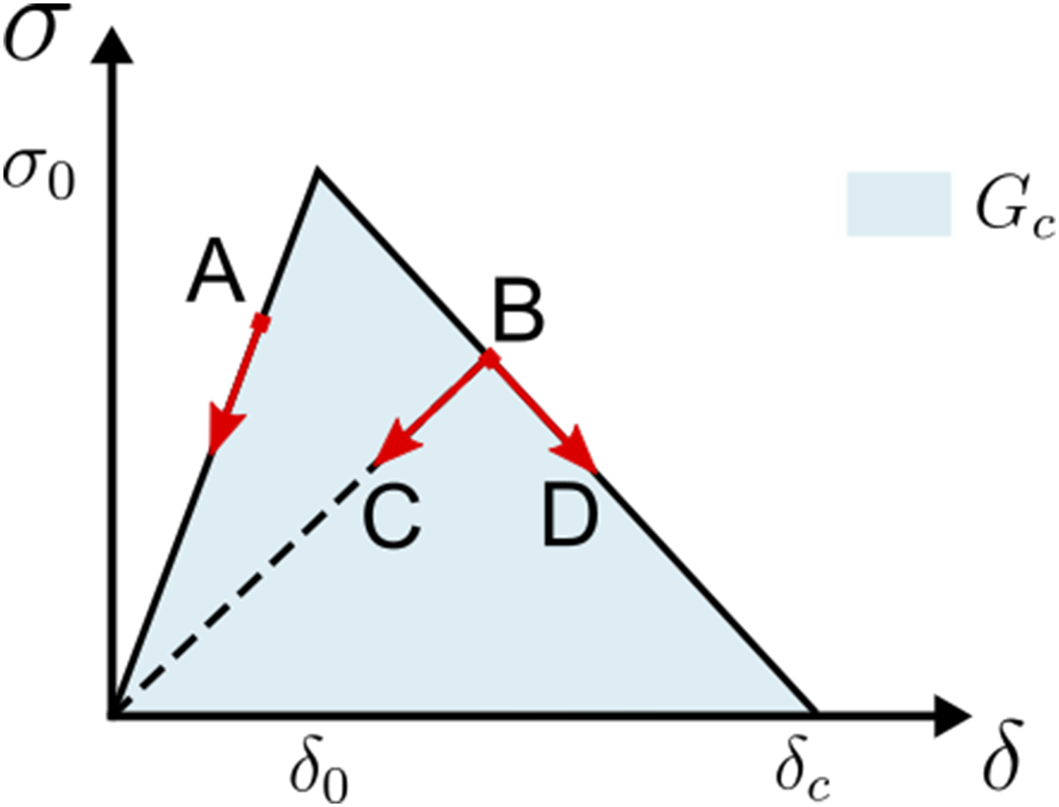

The CZM formulation can be derived asymptotically from a Continuum Damage Model³³ or postulated directly.³⁴ After a initial linear elastic response with very high stiffness K, an internal damage variable d keeps track of the stiffness degradation, until at d = 1 the interface is fully broken and no more stress can be transferred. Although different evolution laws can be defined for d, resulting in different shapes for the σ/δ curve, the key parameters controlling the structural response are the maximum stress σ₀ and the critical strain energy release rate G_c, corresponding to the area under the complete σ/δ curve. 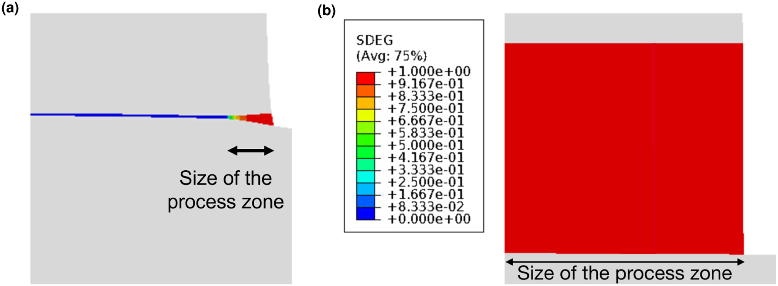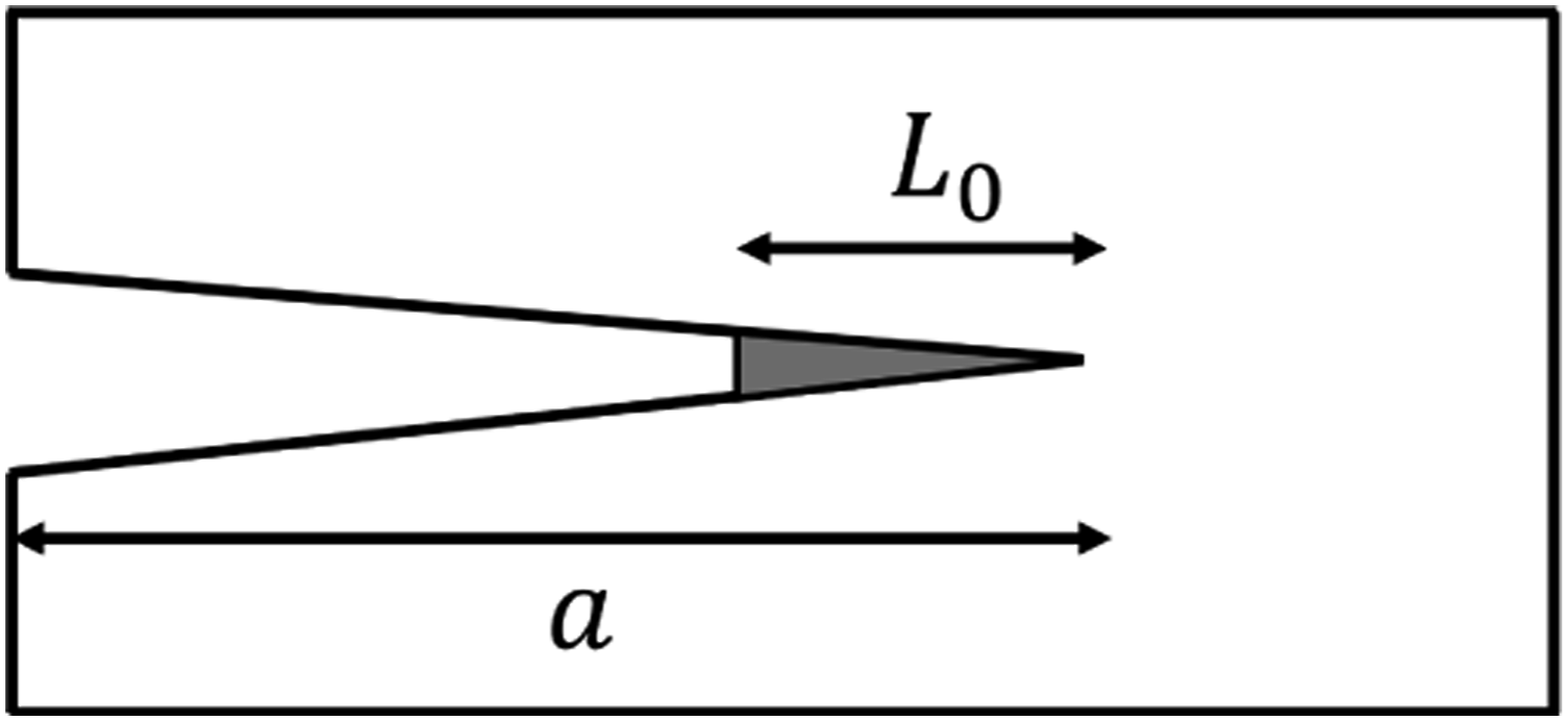Indeed, σ₀ and G_c contribute to fixing the characteristic length of the cohesive zone, called the fracture process zone, that is the length over which the interface goes from perfectly healthy to completely failed³⁵ (see Figure 3). In homogeneous bulk solids, the process zone length L₀ is related to the CZM parameters as follows:

\begin{matrix} L_{0} \propto \frac{δ_{c} E}{σ_{0}} \propto \frac{G_{c} E}{σ_{0}^{2}} \end{matrix}

(1)

Figure 3.

Cracked structure and process zone length.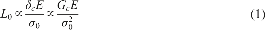

with E the Young’s modulus of the material around the cohesive zone. On the other hand, for slender solids such as beams and plates, the length of the process zone becomes a material-structural property, which also depends on the beam or plate thickness.³⁶

Depending on the relation between the process zone length L₀ and a characteristic dimension a of the structural problem (for instance the crack length, or the ligament size in the case of the T-joint), two cases can be distinguished:

• In small-scale bridging (a/L₀ ≫ 1), the elastic solution is valid almost everywhere, thus an elastic calculation and the application of a criterion as a post-processing enable us to predict the failure conditions for the structure: in the presence of a stress singularity (crack, notch, corner, …) failure is controlled by G_c;

• In large-scale bridging (a/L₀ ≈ 1), both σ₀ and G_c influence the structural response until failure, therefore a structural analysis explicitly describing the nonlinear response of the interface is required.

Estimating the a/L₀ ratio for a given structural problem is paramount for understanding how interface properties control structural failure.

Given the orders of magnitude of the composite transverse stiffness E ∼ 10 GPa, maximum stress σ₀ ∼ 50 − 100 MPa and critical strain energy release rate G_c ∼ 100 − 1000 J/m² for thermosetting and thermoplastic matrix composites, the process zone size is of the order of 0.1-1 mm.³⁶ The characteristic size for the T-joint structure is the width of the ligament, which is of the order of a few mm. This is much smaller than the typical extension of adhesive bonds or inter-ply surfaces. For this reason, large-scale bridging might occur here and both σ₀ and G_c are expected to control structural failure.

In this work, a triangular, mode independent CZM was chosen for its direct control of the input values σ₀ and G_c. The elastic properties and thickness of the CZM are given in Table 3. The Young’s and shear moduli are chosen as typical properties of neat thermoplastic matrix, and the interface thickness corresponds to the thickness of the cohesive elements in the mesh. The initial stiffness of the CZM traction/separation law is computed by dividing the elastic moduli by the thickness of the cohesive elements: this results in a very stiff elastic response of the CZM, which has little influence on the simulation results, while different values of σ₀ and G_c are explored to understand their role on the structural failure.

Table 3.

Cohesive interface dimension and elastic properties.

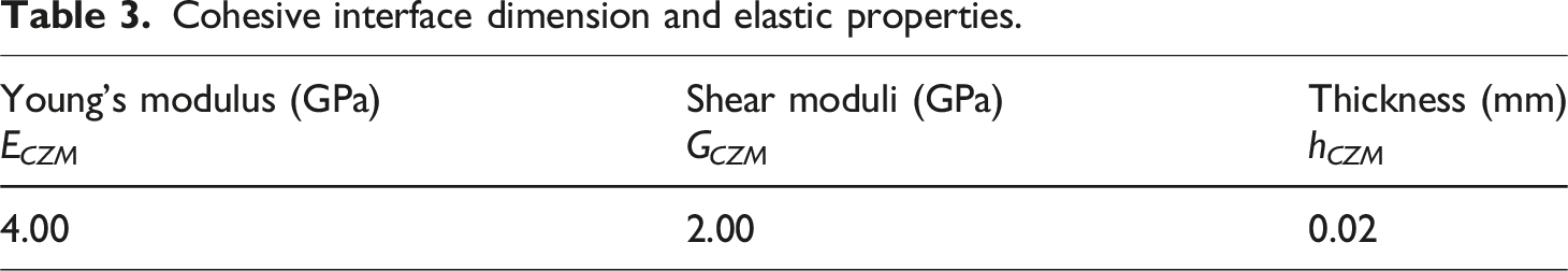
Young’s modulus (GPa) E_CZM	Shear moduli (GPa) G_CZM	Thickness (mm) h_CZM
4.00	2.00	0.02

Although the interface is mostly subjected to mode I in T-joint tests, a certain amount of mode II can be present at the corners of the overmold, depending on its shape and on the amount of bending of the base laminate. Different representations of the CZM mode mixity could modify the initial failure response for cases where the mode II contribution is significant. Investigating this effect would require to define additional parameters for the CZM, namely the maximum shear stress τ₀ and the mode II critical strain energy release rate G_IIc, as well as to choose a law for mixed mode propagation. In this case, the mode independent CZM implemented in Abaqus was considered, which amounts to setting τ₀ = σ₀ and G_IIc = G_Ic = G_c.

Material and structural parameters controlling the T-joint failure

The aim of this work is to explore the mechanical response of the T-joint in a wide range of situations, by modifying:

• The maximum stress σ₀ and critical strain energy release rate G_c of the CZM, chosen to reproduce different bond qualities, possibly associated with different process parameters: their values were chosen to be in the thermosetting - thermoplastic material range, i.e. σ₀ = 10 − 80 MPa and G_c = 350 − 1050 J/m²³⁶;

• The boundary conditions (see Figure 4 for details), chosen to reproduce different solutions for restraining the base laminate during the test. In particular, condition (a) is similar to the in-house test fixture depicted in Figure 1, condition (b) completely prevents bending of the base laminate, while conditions (ci) enable different amounts of bending of the base laminate (i = 1 − 5 mm defines the distance between the edge of the overmold, point A in Figure 5, and the fixture);

• The loading conditions, by setting different values for the load misalignment m = 0 − 5 mm defined in Figure 1. When m = 0, symmetry of the problem is exploited and only half of the T-joint is modeled, introducing symmetry conditions;

• The geometry of the joint, in particular the shape of the overmold and the thickness of the base laminate (see Figures 5 and 6 for details).

The mechanical responses of the different models are analyzed and compared in terms of global quantities of interest, namely the maximum Force per Unit Length (FUL) and the maximum displacement, as well as local damage information, namely the size of the process zone, discussed above. The FUL and the displacement are defined as the nodal quantities on point P on the top of the 2D model, with “length” in direction 2. Although most literature works provide experimental results in terms of strength (that is, force divided by the nominal bond area), the FUL was considered here as it enables a more direct comparison of the maximum load bearing capability for different overmold shapes (and thus different bond areas).

Figure 4.

Boundary conditions.

Figure 5.

Overmold shapes.

Figure 6.

Base laminate thicknesses.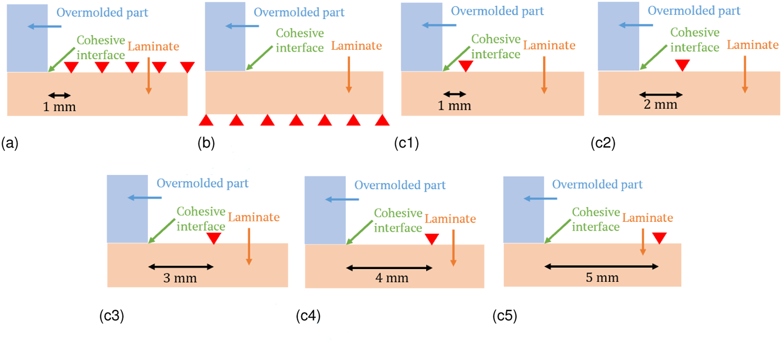

The systematic numerical exploration of the T-joint test features enables us to quantify the effect of each aspect on the load bearing capacity, thus providing key information for the critical interpretation of experimental results provided in the literature, as well as for the design of a new and improved experimental setup, carried out in a forthcoming paper.³²

Numerical aspects

The numerical simulations were carried out using Abaqus Standard 2021 version. The softening material behavior associated to damage and failure can lead to instability and/or loss of uniqueness of the quasi-static solution, resulting in convergence difficulties during the numerical simulations. For this reason, specific user routines were used for simulation control and to define the local search directions for the CZM.

Finite element discretization

Four-nodes bilinear elements (CPE4) were used for both the laminate and the overmold, while cohesive elements (COH2D4) were used for the interface. The size of the elements varies from 0.01 mm (close to the cohesive interface) to 0.1 mm. Based on the à priori estimation of the process zone size,³⁶ as well as on à posteriori observations on the simulation results, this mesh density is largely sufficient to properly resolve the process zone of the CZM and to ensure mesh independent results. The constitutive law used for the cohesive elements is either the native Abaqus implementation, or a user material routine provided by Ref. 37, as it is discussed later.

The computational time for the simulations ranged from approximately 10 to 30 minutes on a computer equipped with two Intel(R) Xeon(R) Silver 4116 CPUs (Skylake) @ 2.10 GHz.

Dissipation-driven approach

The quasi-static FUL versus displacement response of the T-joint structure until failure may involve a snap-back portion (see for example the red line on Figure 7), since elastic energy is stored in both the base laminate and the overmold and dissipated only within the interface between the two. In real displacement-driven experiments, such unstable behavior would result in dynamic crack propagation. Simulating this type of response, and in particular obtaining a reliable value for the maximum FUL, which is the quantity of interest in this work, is particularly challenging.

Figure 7.

Increment of energy dissipation.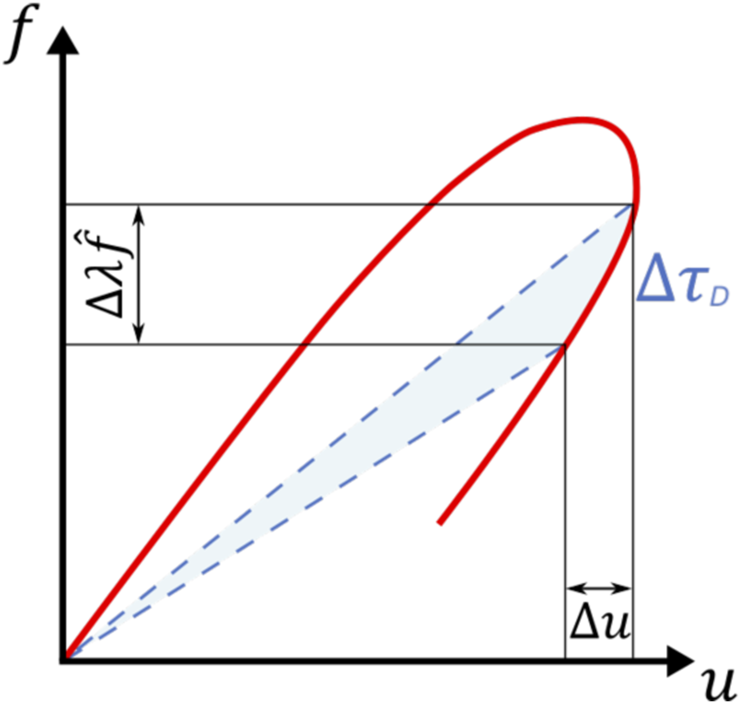

In the presence of snap-back, standard displacement-driven quasi-static simulations would result in lack of convergence. A typical solution is to introduce a viscous regularization term, however this artificially increases energy dissipation in the system, thus modifying the problem at hand and potentially overestimating the maximum FUL. A full dynamic simulation of the failure process would result in a high computational cost due to the need for a very small time step.

An alternative solution, adopted here, is to remain in a quasi-static setting and to capture the whole structural equilibrium path, including the maximum FUL, by modifying the simulation driving strategy. In particular, we choose to impose an increment of dissipated energy, which is a monotonically increasing quantity (see the blue area in Figure 7). The dissipation-driven approach described below was proposed by Refs. 38 and 39, and adapted for an Abaqus implementation in Ref. 40 It is briefly recalled here.

Consider a discretization of a solid Ω, the nodal displacements are denoted u, and the equilibrium equation is written as:

\begin{matrix} λ \hat{f} - f^{int} (u) = 0 \end{matrix}

(2)

Where f^int is the vector of internal nodal forces, $f^{ext} = λ \hat{f}$ is the vector of external forces, defined through a scalar load multiplier λ and a proportional loading direction $\hat{f}$ . If both displacements and load multiplier are allowed to vary, the solution to look for is (u, λ), involving N + 1 unknowns (where N is the number of nodal degrees of freedom). Equation (2) involves only N equations, thus an extra equation, the driving condition, needs to be defined. In particular, setting ${\dot{τ}}_{D}$ as the imposed rate of energy dissipation in the structure leads to the following condition:

\begin{matrix} D - {\dot{τ}}_{D} = 0 \end{matrix}

(3)

Where $D = P - \dot{V}$ is the rate of dissipated energy, P is the power of the external forces and $\dot{V}$ is the elastic potential energy rate. Expressing equation (3) in terms of the problem unknowns for the case of a linear elastic problem, with damageable constitutive laws and no residual stresses, leads to

\begin{matrix} \frac{1}{2} (λ {\dot{u}}^{T} - \dot{λ} u^{T}) \hat{f} - {\dot{τ}}_{D} = 0 \end{matrix}

(4)

which can be integrated using a forward Euler scheme, yielding:

\begin{matrix} \frac{1}{2} [λ_{n} (Δ u^{T}) - Δ λ u_{n}^{T}] \hat{f} - Δ τ_{D} = 0 \end{matrix}

(5)

where (u_n, λ_n) are the values at the beginning of the increment, (Δu, Δλ) are the displacement and load increments, and Δτ_D represents the dissipation increment, depicted by the blue area in Figure 7. Such condition must be solved together with the equilibrium equations in order to find the next point of the equilibrium path.

Adding the driving constraint to a black-box finite element code for general loading conditions may be complex, as equation (5) involves all of the nodal degrees of freedom work-conjugate to the external loading vector $\hat{f}$ . For this reason, here we choose to control a single degree of freedom $\bar{u}$ of the problem, which gives.

\begin{matrix} u^{T} λ \hat{f} = \bar{u} λ \bar{f} = \bar{u} λ \end{matrix}

(6)

and we introduce the extra (scalar) driving constraint equation through an Abaqus User Element (UEL). In particular, the load multiplier λ is stored in an unused degree of freedom for the element, for instance, a rotational degree of freedom for problems modeled with only volumetric or truss elements. As energy dissipation does not occur until damage activation in the CZM, a displacement-based driving constraint is also implemented in the UEL to handle the first part of the simulation. The UEL described above and used here was implemented in Ref. 40 It is made available here as supplementary material⁴¹ and detailed in the Appendix.

In the results presented here, a rigid body constraint was imposed on the top edge of the structure. A short truss element (involving no rotational degrees of freedom and adding very little stiffness to the overall structural problem) was attached on one end to the reference point of the constraint, and on the other end to the UEL.

Choice of the search direction for the Newton-Raphson algorithm

During the simulations with the native Abaqus implementation of the CZM, convergence problems appeared for some of the simulations. In particular, an oscillating behavior of the Newton-Raphson algorithm was observed in the cases involving a chamfer and bending conditions, where two possible evolutions of the cohesive zone were observed (namely, increased damage and displacement jump at the free edge, where crack initiation has already taken place, vs propagation further into the ligament).

This sort of situations, where different degradation mechanisms are in competition, can arise even in relatively simple crack propagation problems, and is associated to the loss of uniqueness of the equilibrium path. To the authors’ knowledge, there is no systematic solution for this difficulty, and the full range of possible solutions cannot generally be recovered through a simple incremental-iterative approach. However, a different choice of the search direction for the Newton-Raphson algorithm can in some cases help finding a specific branch of the solution.

As it was studied in details in Ref. 37, for a given point along the softening branch of the σ/δ curve two increments are possible, associated to the same applied stress: in the first, the displacement and the damage increase, and the tangent stiffness is negative, while in the second the displacement decreases, the damage remains constant, and the tangent stiffness is positive (paths BD anc BC on Figure 2, respectively). Thus, even considering a single cohesive element, the equilibrium path is unique if the displacement jump is imposed, and not unique if the stress is imposed. Unlike Ref. 37, we do not believe that one equilibrium path is ‘more physical’ than the other.

A cohesive element within a structure is neither under imposed displacement nor imposed stress conditions, as its response during an increment depends on the overall driving conditions, as well as on the local stiffness and load redistribution within the structure. At the beginning of a given increment, without a priori information, the two equilibrium paths are equally possible, and two different search directions can be defined for each element. A negative initial tangent stiffness, as in the native Abaqus implementation of CZM, tends to privilege the increase of displacement and damage within an already damaged element, while a positive initial tangent stiffness, as in the UMAT provided by Ref. 37 as supplementary material,⁴² tends to privilege a constant damage and a decrease of displacement.

Both CZM implementations were tested in the simulations described here. While, in some cases, both led to convergence with analogous global force/displacement response, the UMAT provided in Ref. 42 seemed to perform better when the overall response involved a competition between two active CZM zones, thus it was used for some of the simulations discussed in this paper.

Results & discussion

The modeling approach presented above is used here to simulate a wide range of situations, encompassing different choices of interface parameters, boundary and loading conditions and specimen geometry. To the authors’ knowledge, no systematic numerical investigation of the features of the T-joint test was carried out before. The results presented here enable us to clarify the role of each aspect of the problem on the performance of the assembly, as well as to provide indications to improve the process of design, sizing and experimental characterization of overmolded structures.

Experimental Information

Although this work is exclusively numerical, a preliminary validation of the approach is carried out by considering experimental results from the literature and from tests carried out by CETIM.

Most publications do not provide full load-displacement curves, but only maximum loads or maximum stresses at failure, which range between 2 and 12 MPa in Ref. 8 and between 20 and 35 MPa in Ref. 6 for a wide variety of materials and overmold shapes.

Experimental tests were carried out at CETIM on T-joints made of the material system presented above. As they were part of a confidential study, the results cannot be published here, but some information relevant for validation is discussed below.

The first key point to be pointed out is the relevance of load and displacement experimental information for validation purposes. In the experiments at CETIM, two different testing machines were used, with capacities of 10 kN and 100 kN, respectively, yielding two families of load-displacement curves with significantly different stiffness. Indeed, the crosshead displacement includes two displacement contributions: the first is associated to the T-joint, and the second results from the compliance of the testing machine itself. As the T-joint is short, thus very stiff, the compliance of the testing machine is a significant portion of the crosshead displacement. For this reason, experimental displacement values can change significantly when using different testing machines, and simulated displacements are expected to be much smaller than the experimental ones. Changes in the stiffness of the T-joints, as can occur for instance due to different boundary conditions of the base laminate, can be masked by the compliance of the testing machine during experiments, but they are visible when comparing displacements between simulations, which describe the response of the T-joint alone. The load measured by the load cell, on the other hand, corresponds to the load seen by the T-joint, thus it can be simply divided by the interface dimension in the x₂ direction (42 mm in these experiments) to obtain the experimental counterpart of the FUL computed in the simulations. Only the FUL can be pertinently compared between experiments and simulations.

In experiments at CETIM, the maximum forces obtained were very dispersed. In particular, for the straight joint geometry, maximum loads between 2 and 5 kN (stresses between 12 and 30 MPa) were found, and the corresponding FUL range is reported in green in Figures 10 and 13 for easy, at a glance comparison.

The second aspect is related to the failure location after testing. Different failure locations were observed in the literature (see for example in Ref. 6). In experimental tests by CETIM, final failure often occurred at the interface between the laminate and the overmold, that is where the CZM was introduced in the simulations. Some portions of the overmold were also visible in the case of chamfer joint, showing a possible deviation of the main crack within the overmold: this cannot be represented by the model proposed here, and it would require to include additional CZM within the overmold or to introduce numerical techniques enabling the crack direction to evolve, such as X-FEM or phase-field models.

Role of the bond properties

Different bond properties are translated in the model as different values of the CZM parameters σ₀ and G_c. These indirectly represent different choices of materials for the laminate and the overmold, and in particular the compatibility of the different matrices, but also different parameters of the manufacturing process (injection temperature and pressure, flow conditions, time, …) which lead to different adhesion properties at the interface between the laminate and the overmold.

All simulations in this Section are carried out on a straight T-joint with simple laminate thickness, using boundary condition (a) and aligned loading, which is taken to represent a typical experiment.⁸ The results are presented in Figures 8–10.

Figure 8.

FUL versus displacement curves, 1 - blue line (short process zone), 2 - orange line (medium process zone), 3 - yellow line (long process zone) [straight joint, simple thickness, boundary condition a].

Figure 9.

Damage contour plot for two different sets of CZM parameters (curves 1 and 3 of Figure 8), leading to small-scale bridging (a) and large-scale bridging (b) conditions. 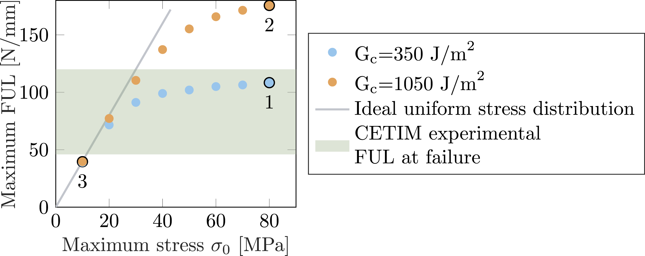In both (a) and (b), half of the T-joint is represented due to the symmetry of the problem, d = SDEG is the damage variable of the CZM, whose value is 1 when the interface is fully broken; (a) Small-scale bridging - curve 1 of Figure 8 [straight joint, G_c = 350 J/m², σ₀ = 80 MPa, simple thickness, boundary condition a] (b) Large-scale bridging - curve 3 of Figure 8 [straight joint, G_c = 1050 J/m², σ₀ = 10 MPa, simple thickness, boundary condition a].

Figure 10.

Influence of the cohesive parameters on the global behavior [straight joint, G_c = 350 − 1050 J/m², σ₀ = 10 − 80 MPa, simple thickness, boundary condition a]. Points 1 to 3 correspond to the full response curves given in Figure 8.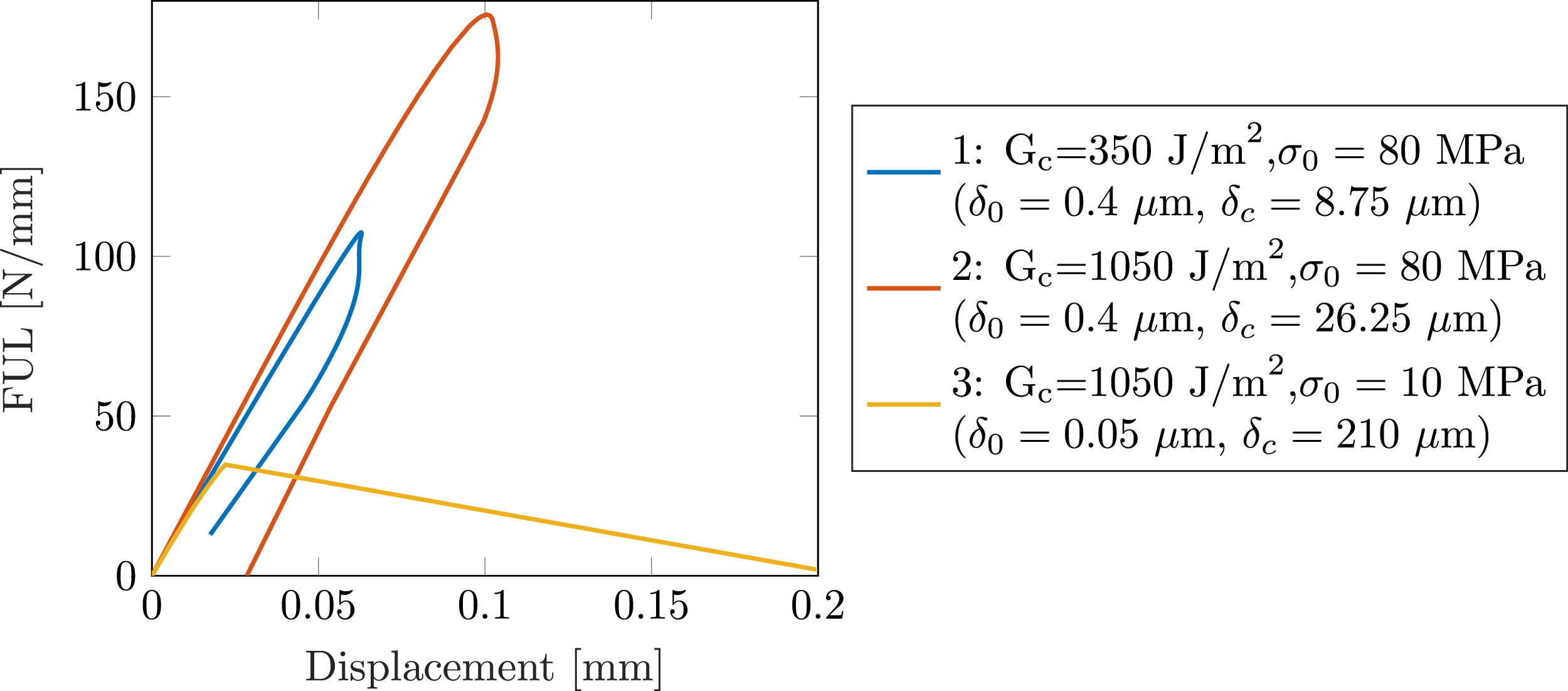

The range of CZM parameters considered here gives rise to a wide variety of quasi-static equilibrium curves, depicted in Figure 8. Differences between these curves reside in the maximum FUL value, with a 80% decrease between curves 2 and 3 of Figure 8, but also in the shape of the post-peak response. In particular, most of the considered examples display the anticipated snap-back instability (curves 1 and 2 of Figure 8, as well as most of the curves presented in the rest of the paper), while for some sets of parameters the response was observed to be stable under imposed displacement conditions (curve 3 of Figure 8). A higher value of the maximum FUL corresponds to a higher load bearing capacity of the assembly, which is desirable for industrial applications. On the other hand, the post-peak snap-back implies an abrupt failure scenario, where the energy released in the form of a dynamic excitation can lead to further structural damage. Unfortunately, the best-case scenario, that is a high maximum FUL accompanied by a stable post-peak response, is practically impossible to reach with CZM parameters in the typical range for composite interfaces.

The stability of the post-peak response can be related to the ratio between the width of the overmold ligament and size of the process zone L₀, whose dependence on the CZM parameters is given in equation (1). The size of the process zone for curves 1 and 3 of Figure 8 is depicted in Figure 9(a) and (b), respectively. In both cases, half of the T-joint is represented for symmetry, and the contour plot of the damage variable (d = SDEG in Abaqus) is shown for the interface, at the moment when the most damaged element reaches d = 1. In small-scale bridging (Figure 9(a)), a small process zone is established before the crack propagates along the ligament. Complete failure of the first cohesive elements reduces the section of interface through which load can be transferred: in a quasi-static equilibrium setting, this abruptly decreases the FUL and unloads the laminate and overmold. Both FUL and displacement decrease quickly, resulting in the unstable snap-back response of curve 1. In large-scale bridging (Figure 9(b)), on the other hand, nearly homogeneous displacement jump and stress level are reached before the crack is fully initiated. The maximum FUL reached by the T-joint is much lower, as it is limited by the low maximum stress σ₀ at the interface. The subsequent decrease of FUL and displacement of the laminate and overmold are much more gradual and distributed along the whole interface section, resulting in the stable post-peak response observed in curve 3. In general, the maximum FUL is related in a complex way to both G_c and σ₀.

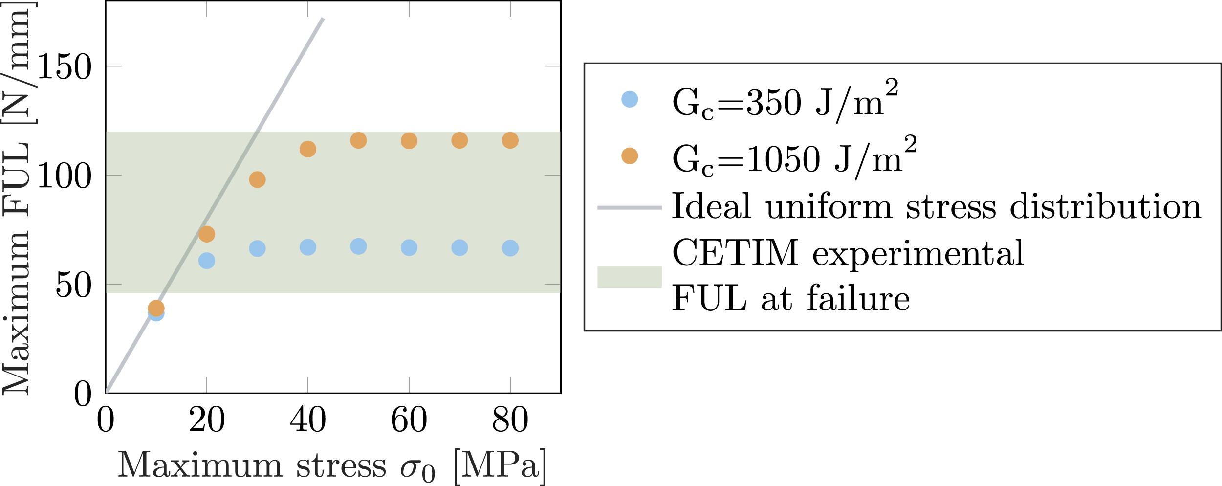
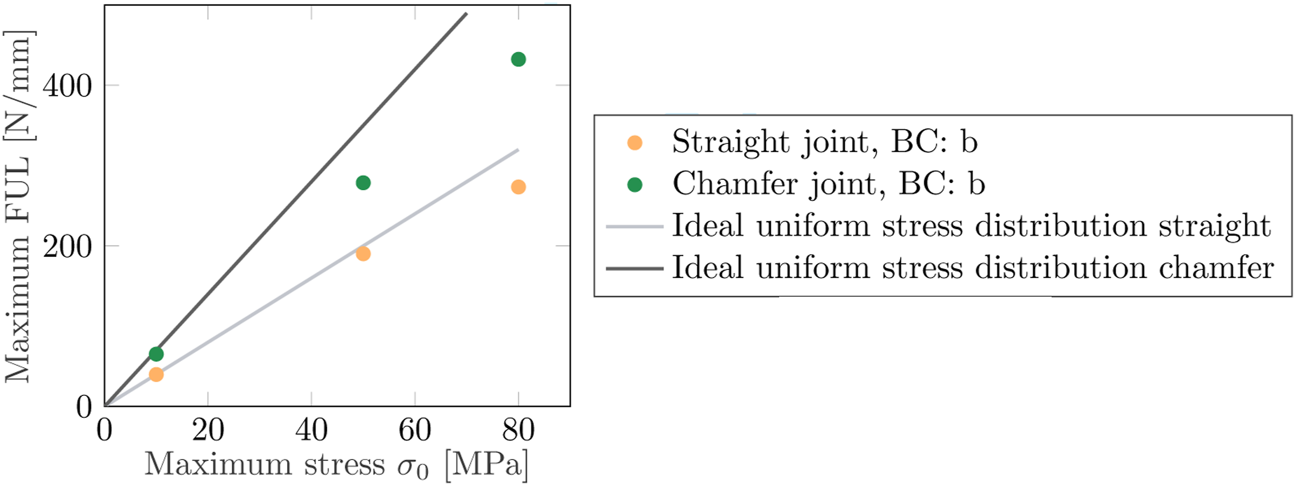
In order to clarify the role of each parameter, a synthesis of the maximum FUL values for different (G_c, σ₀) couples is depicted in Figure 10. The Figure also reports the FUL range from CETIM’s experiments (in green), as well as a grey line representing the FUL associated to an ideal uniform stress distribution, obtained by multiplying the maximum stress σ₀ at the interface by the width of the ligament. This FUL would be reached if no stress concentration was present to decrease the load bearing capacity of the T-joint.

As expected, the maximum FUL increases with both σ₀ and G_c. However, the importance of each parameter is different in different zones of the graph, as the ratio a/L₀ goes from large-scale to small-scale bridging conditions, moving from the left to the right side of the graph. Indeed:

• In small-scale bridging conditions (right side), the maximum FUL is essentially controlled by G_c, as well as by the severity of the stress concentration, which in turns depends on the boundary and loading conditions and on the geometry, as it is discussed later;

• In very large-scale bridging conditions (left side), a nearly homogeneous stress is reached in the CZM during process zone development, thus the maximum FUL is controlled by σ₀ and the ideal value associated to uniform stress distribution is approached;

• In intermediate situations, both σ₀ and G_c play a role in determining the maximum FUL.

For this reason, a full characterization of the properties of the interface between the base laminate and the overmold should include both the maximum stress, or strength, σ₀ and the critical strain energy release rate G_c.

The maximum FUL values provided by some of the simulations represented in Figures 8 and 10 are in the same range as the available experimental results, providing a preliminary validation of the proposed numerical approach. Since the boundary and loading conditions play a significant role in the load bearing capacity of the T-joint, as it is discussed in the following, pertinent numerical-experimental comparisons require a finer control of such conditions in a real experiment. The design of an appropriate experimental setup, as well as further numerical-experimental comparisons, will be the subject of a forthcoming paper.³²

Role of the loading conditions

As it is discussed in the Introduction, no normalized test exists for T-joint specimens, thus similar in-house fixtures were developed by different research groups working on the subject.^{6,8–10,14,18,20,21,25–28} A clear description of the boundary conditions and load application is generally not provided in these works, particularly concerning the system enabling to retain the base laminate, as well as the alignment of the load with respect to the overmold. However, loading conditions are expected to have a paramount role on the stiffness of the FUL/displacement response and, more importantly, on the stress concentration which controls the maximum FUL under small-scale bridging conditions. Understanding the role of loading conditions enables to critically interpret the experimental results available in the literature and to provide recommendations to improve the experimental protocols. In this sense, the results presented below provide numerically-motivated interpretations and recommendations for T-joint test setups, constituting a numerical counterpart to recent experimental works such as Ref. 28.

Role of the boundary conditions

Three types of boundary conditions are simulated here (see Figure 4):

• Condition (a), where a portion of the top surface of the base laminate is blocked, is supposed to represent an experimental setup analogous to Figure 1;

• Condition (b), where the bending of the base laminate is completely prevented by blocking the displacement of its bottom part, for instance by gluing the T joint to a thick and rigid support;

• Conditions (ci), where different amounts of bending are authorized, by blocking the displacement of a single node at a distance i from the end of the overmold.

A first illustration of the influence of boundary conditions on the FUL versus displacement response is given in Figure 11, fixing the CZM parameters (G_c = 1050 J/m², σ₀ = 80 MPa) and the T-joint geometry (straight joint, single laminate thickness). As it can be observed in the Figure, both stiffness and maximum FUL decrease as the amount of bending increases, with a FUL reduction of around 50% between the (b) and (c5) boundary conditions.

Figure 11.

Influence of the boundary conditions [straight joint, G_c = 1050 J/m², σ₀ = 80 MPa, simple thickness, boundary conditions a, b, c1-c5].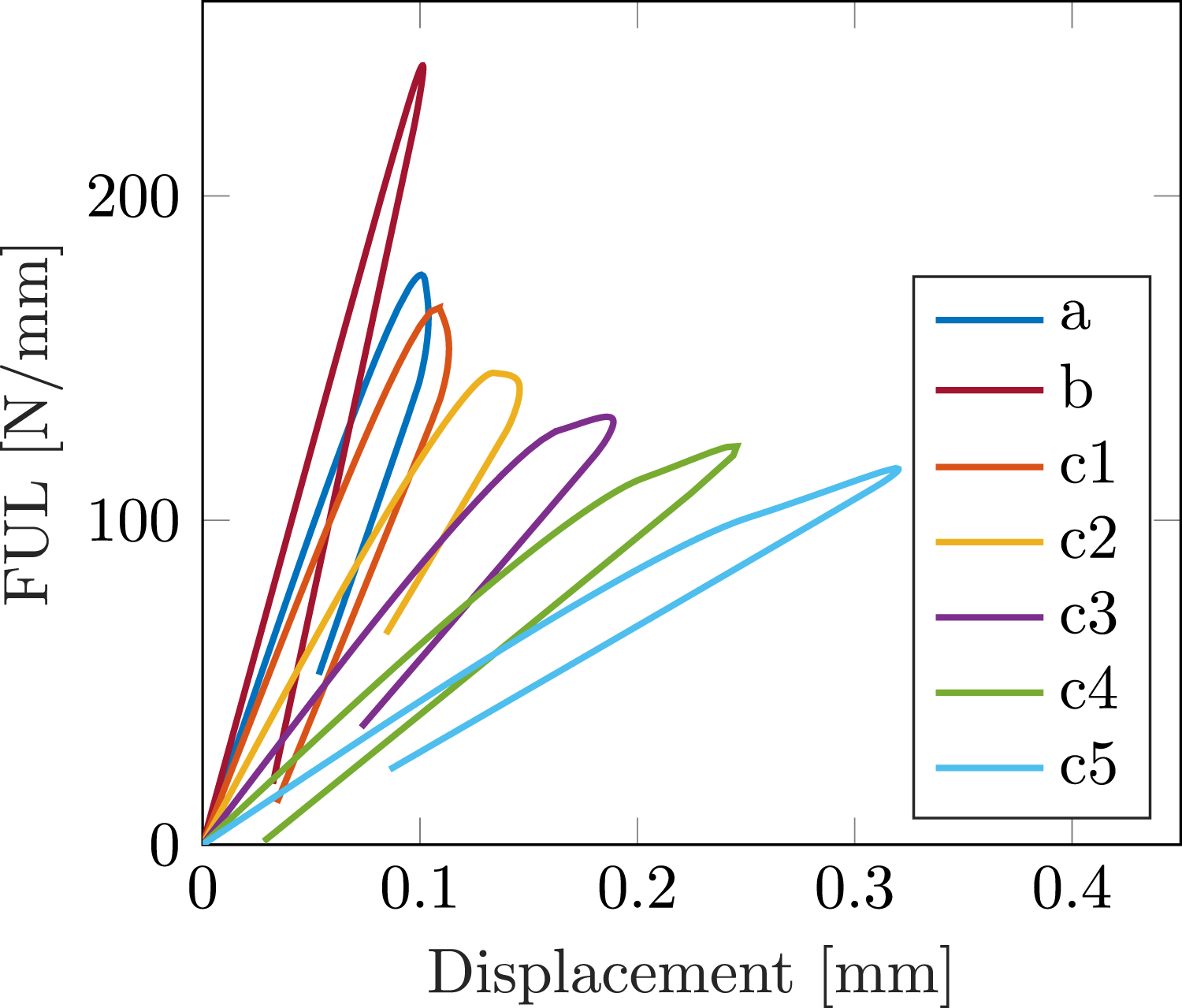

As the T-joint alone, and no testing machine, is described in the simulations, it is pertinent to compare displacements for different boundary conditions. Two main contributions determine the T-joint displacement: bending of the base laminate and elongation of the overmold. As such, increasing the bending of the base laminate leads to larger overall displacement, which decreases the stiffness. The interface zone, on the other hand, is very thin, for this reason its contribution to displacement becomes visible only during failure.

The second, and more important, effect of bending is to induce a more severe stress concentration at the corner of the overmold, which in turn decreases the maximum FUL. While being less severe than conditions (ci), condition (a) authorizes some amount of bending, thus leading to lower stiffness and maximum FUL than condition (b), where bending is completely prevented.

The link between bending and stress concentration can be visualized by looking at the symbol plots of the maximum principal stresses before interface damage starts to occur for conditions (a) and (b), depicted in Figure 12. This type of plot provides complementary information with respect to more classical color plots, as it enables one to visualize the direction of the stress flow lines in the structure, which can be read and interpreted similarly to the flow of a liquid along a channel. In both cases, the flow lines are directed from the overmolded part, where loading is applied, towards the boundary condition, where the reaction forces associated to the blocked displacement develop. In boundary condition (a), this results in the stress flow turning around the free corner of the overmold and engendering significant stress concentration, while in boundary condition (b) the stress flow lines are nearly vertical and suffer only a little perturbation by the free corner. Given this fundamental difference, reducing the distance between the blocked nodes and the base of the overmold, as in condition (a), appears not to be enough to fully eliminate bending of the base laminate and its influence on failure. Although little description of the test setup is provided in most experimental works on T-joints, it is expected that most of them involve some amount of uncontrolled bending, which is shown here to have a strong influence on the load bearing capacity of the assembly.

Figure 12.

Symbol plots illustrating the flow lines of the maximal principal stresses for two different boundary conditions [straight joint, G_c = 1050 J/m², σ₀ = 80 MPa, simple thickness]; (a) Boundary condition (a); (b) Boundary condition (b).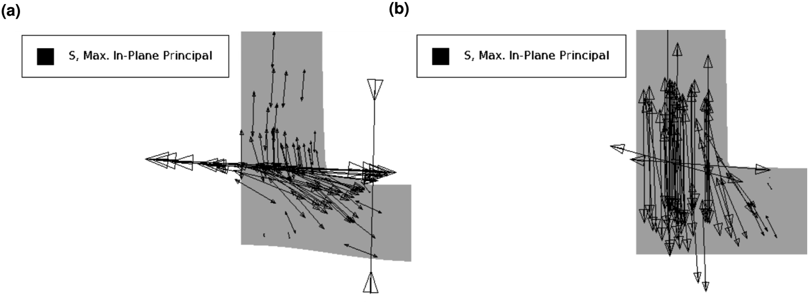

As the stress concentration is also influenced by the CZM parameters through the definition of the process zone size, it is interesting to explore how these two aspects of the problem interact. For this, a synthesis of the maximum FUL for different (G_c, σ₀) couples under boundary condition (c5) is depicted in Figure 13. This figure can be directly compared to Figure 10, where the same results are depicted for boundary condition (a). Comparing the maximum FUL in the two Figures:

• In small-scale bridging conditions (right side), the maximum FUL values are significantly smaller for condition (c5) than for condition (a), highlighting a more severe stress concentration when more bending is allowed;

• In very large-scale bridging conditions (left side), the maximum FUL is analogous for the two boundary conditions, since the initial stress concentration is homogenized during development of the very large process zone;

• The transition between the two regimes is much faster for condition (c5), where the range of CZM parameters for which both σ₀ and G_c play a role in the maximum FUL is smaller.

Figure 13.

Influence of the cohesive parameters on the global behavior [straight joint, G_c = 350 − 1050 J/m², σ₀ = 10 − 80 MPa, simple thickness, boundary condition c5].

Role of the load alignment

Another aspect worth investigating with regard to the loading conditions is the impact of misaligned loading. Classical test setups are hyperstatic, thus load misalignment can be generated by geometry defects in the specimen or in the alignment of the testing machine. Uncontrolled load misalignment is shown here to have a very significant impact on the load bearing capacity of the T-joint.

Load misalignment breaks the symmetry of the problem, therefore the whole geometry is taken into account in the simulations. Four different cases of misalignment are studied: the loading in blue is centered and serves as the reference (m = 0); the orange, yellow, purple ones are misaligned setting m to 0.5 mm, 1 mm, 5 mm respectively. For 5 mm, where the point P is outside of the top surface of the overmold, a highly rigid beam is added horizontally to the top of the structure before connecting to the vertical truss used for load application. For all simulations, the CZM parameters (G_c = 1050 J/m², σ₀ = 80 MPa), the T-joint geometry (straight joint, single laminate thickness) and the boundary condition (b) are fixed. The corresponding FUL versus displacement curves are presented in Figure 14.

Figure 14.

Influence of misaligned loading [straight joint, G_c = 1050 J/m², σ₀ = 80 MPa, simple thickness, boundary condition b].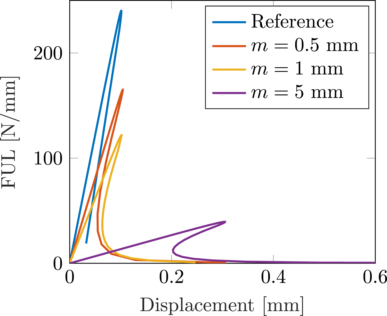

The maximum FUL is significantly influenced by the misalignment: even with a 0.5 mm shift, the result decreases by more than 30%. This reduction reaches more than 80% when the offset is set to 5 mm. Indeed, misalignment introduces a moment in the loading seen by the interface between the laminate and the overmold. This leads higher stresses on one of the corners of the overmold, which largely diminishes its maximum load bearing capacity.

Recommendations for improvements of the experimental testing protocols

As it was observed in the Sections above, the loading conditions, and in particular bending of the base laminate and load misalignment, have a first order influence on the measured performance of the T-joint assemblies, especially under small-scale bridging conditions. This provides a first explanation for the variability of experimental results, both within a single literature work and between different works. More importantly, this shows that it is impossible to directly extrapolate maximum stress or maximum load values obtained from coupons to the sizing of a real structure, as the laboratory tests are unlikely to be perfectly representative of the real loading conditions. These difficulties were recently pointed out in Ref. 28, which provided qualitative recommendations for the improvement of the T-joint test protocol based on an experimental investigation. The numerical results presented here enable us to quantify the influence of each aspect.

In view of these results, experimental tests on coupons should not be used to directly evaluate the performance of a T-joint assembly, but to identify CZM properties and to validate structural models, which can then be used to predict the performance of assemblies under different real-life loading conditions. With this in mind, further developments of this work consist in the definition of appropriate tests for the identification of σ₀ and G_c, as well as for the validation of the model discussed here.²³ In particular, the numerical results presented in this work provide a guide for the design of a new test setup enabling a fine control of the boundary conditions and of the load alignment. It will be the subject of a forthcoming publication.³²

Role of the specimen geometry

The geometry of the T-joint, defined in the design phase, interacts with the other factors discussed above to determine the performance of the assembly. An exhaustive exploration of the design space is besides the scope of this work, thus only some tendencies are explored by modifying the thickness of the base laminate, as well as the shape of the overmold. The methodology proposed in this work can easily be used to explore other configurations of interest.

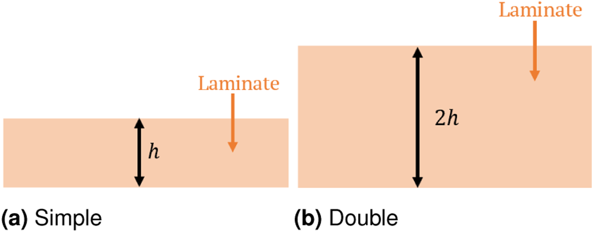
Role of the thickness of the base laminate

Modifying the thickness of the base laminate significantly modifies its bending stiffness, thus changing the sensitivity of the T-joint to the boundary conditions. As an illustration, Figure 15 depicts the FUL versus displacement responses for different boundary conditions of a T-joint analogous to the one of Figure 11, but whose base laminate has double the thickness. The results from Figure 11 are also reported in gray on Figure 15 for ease of comparison. As it can be observed, doubling the thickness of the base laminate increases the overall stiffness and the maximum FUL, while significantly reducing the consequences of changing the distance between the bending supports (conditions (c1) to (c5)). Increasing the thickness of the base laminate is a convenient way to minimize the influence of the boundary conditions applied to the base laminate, as it was also pointed out in Ref. 28.

Figure 15.

FUL versus displacement responses for different boundary conditions and double base laminate thickness [straight joint, G_c = 1050 J/m² σ₀ = 80 MPa, double thickness, boundary conditions c1-c5]. In grey the data for single base laminate thickness for comparison (from Figure 11).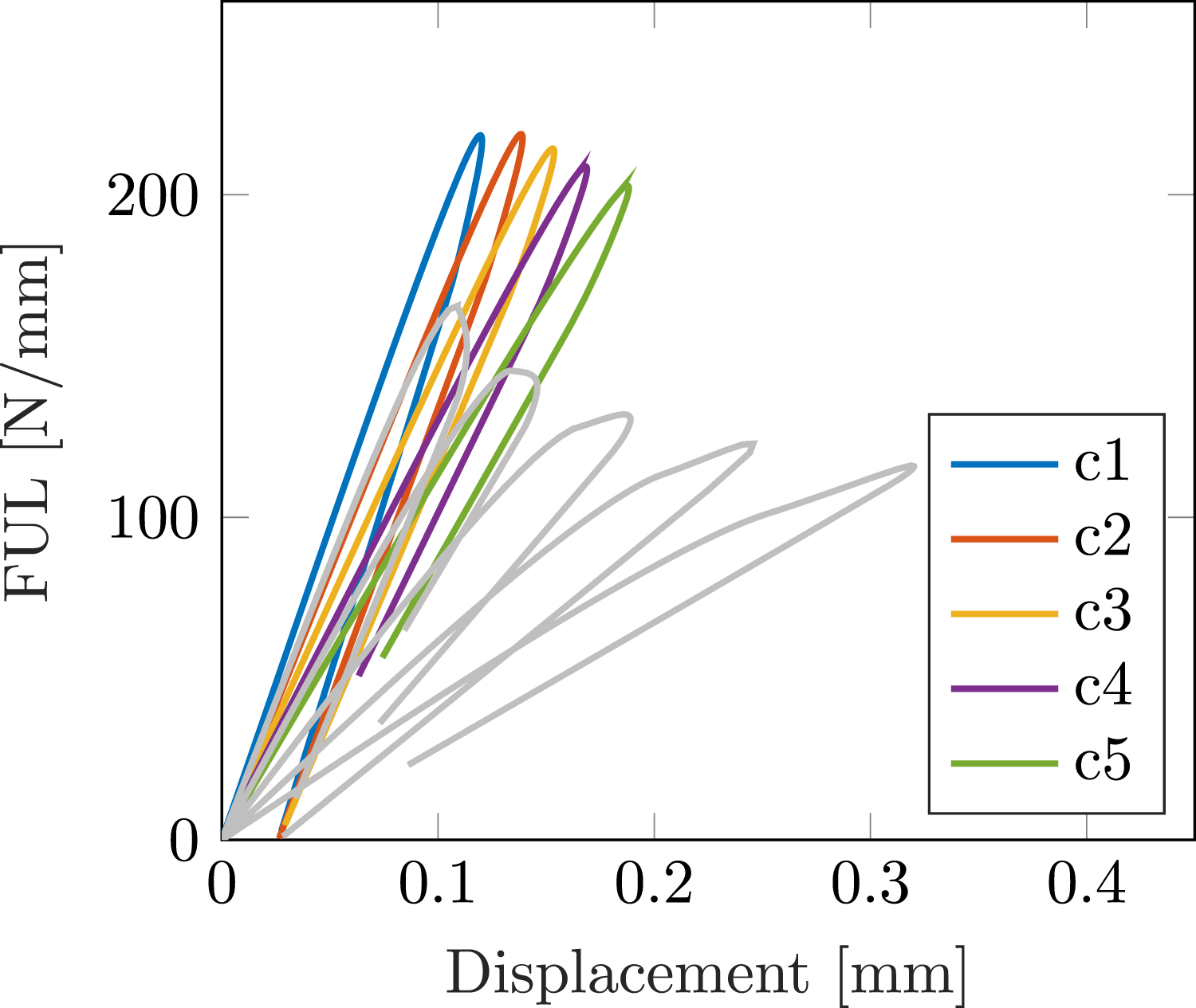

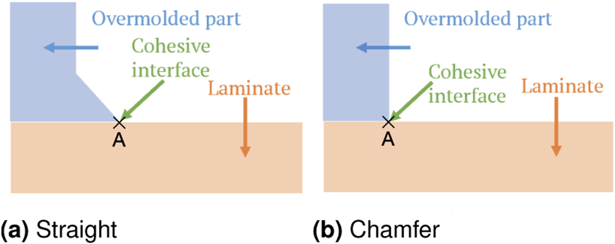
Role of the geometry of the overmolded part

The contact surface between the laminate and the overmold can be increased by adding a chamfer to the overmold. As the load bearing capacity of the T-joint depends in a complex way on the structural problem, the increase in the ligament width does not result in a proportional increase of the maximum FUL, but it can modify the way the interface crack initiates and evolves during loading under different boundary conditions. A single geometry variation, namely a triangular chamfer providing an extra 1.5 mm interface width on either side, was considered here to illustrate these effects. Other chamfer geometries could be investigated with the same approach.

When bending is prevented, as in boundary condition (b), the presence of the chamfer further reduces the stress concentration at the corner of the overmold. As a result, the damage onset location moves from the free corner to the center of the specimen, as it can be observed in Figure 16. Contrary to the previous illustration, Figure 9(a), where damage initiated at the free edge of the overmold (right hand of the picture), here the maximum value of d is on the left of the picture, which corresponds to the center of the specimen due to symmetry. Figure 17 compares the maximum FUL values for straight and chamfer geometries, boundary condition (b) and a few values of CZM parameters: while the maximum FUL is higher for the chamfer case, its distance from the theoretical ideal is greater than that of the straight joint, since the tip of the chamfer is not stiff enough to ensure a uniform stress distribution on the whole surface in contact with the base laminate.

Figure 16.

Damage contour plot for a chamfer joint and no bending (boundary condition (b)) [G_c = 1050 J/m², σ₀ = 80 MPa, simple thickness]. Half of the T-joint is represented due to the symmetry of the problem, d = SDEG is the damage variable of the CZM, whose value is 1 when the interface is fully broken.

Figure 17.

Influence of the geometry of the overmold on the global behavior [G_c = 1050 J/m², simple thickness].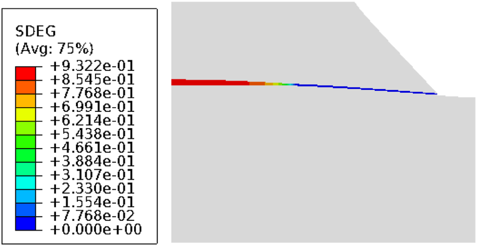

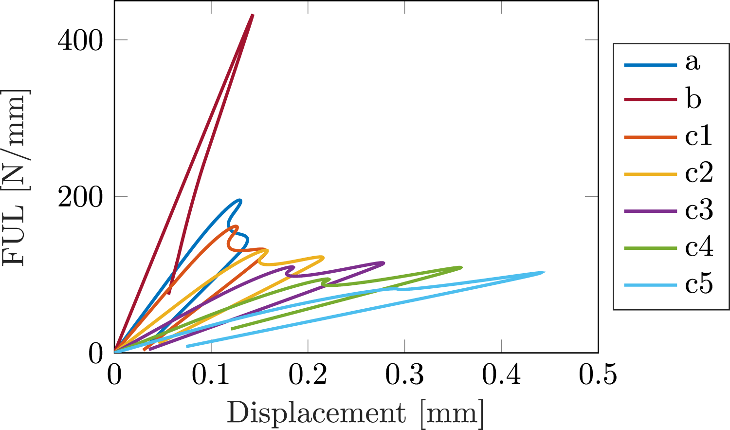
When bending is authorised, as in boundary conditions (ci), damage onset occurs at the corner of the overmold. However, differently from the case of the straight joint, damage propagation occurs in three phases, as illustrated in Figure 18. During the first load increase, damage starts developing at the free corner of the overmold and it progresses towards the center of the T-joint, but no fully failed cohesive elements are observed (Figure 18(a)). During the first snap-back observed in the yellow curve of Figure 19, the tip of the damage zone stagnates below the chamfer and the process zone length does not increase, but damage continues to increase at the free corner of the overmold, leading to complete failure of the cohesive elements close to the free boundary and to full separation of the chamfer tip from the substrate (Figure 18(b)). Finally, damage propagation towards the heart of the T-joint resumes, leading to complete failure of the specimen (Figure 18(c)). These three phases of damage are observed in most cases involving the chamfer geometry, and they are materialized in the FUL versus displacement curves by the presence of two FUL peaks, as observed in Figure 19. The competition between crack advance within the interface and damage increase in the partially damaged elements generated convergence difficulties in the simulation, which could be overcome by modifying the local search direction in the cohesive elements.

Figure 18.

Damage contour plot [chamfer joint, G_c = 1050 J/m², σ₀ = 80 MPa, boundary condition c2].

Figure 19.

Influence of boundary conditions [chamfer joint, G_c = 1050 J/m², σ₀ = 80 MPa, simple thickness].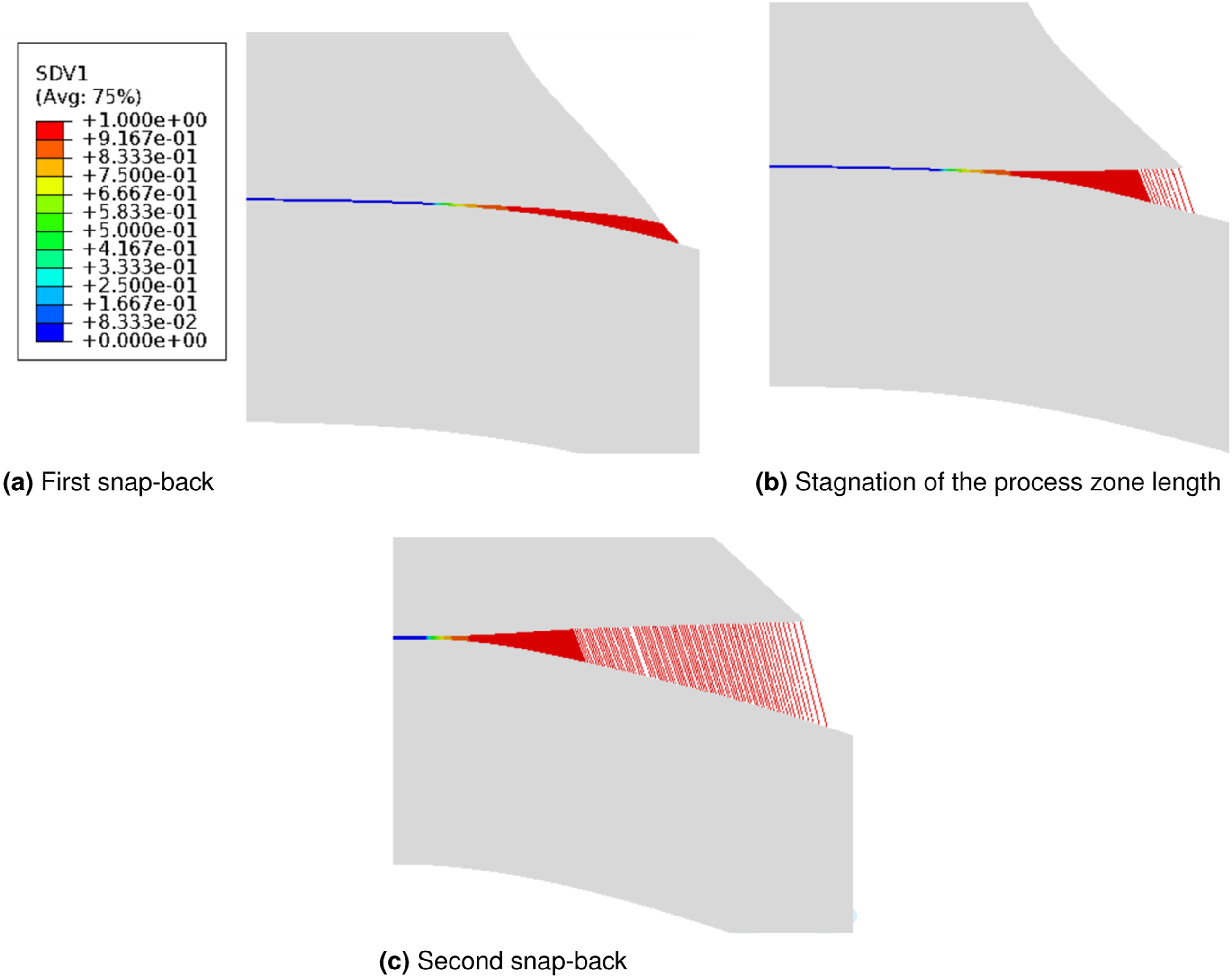

The reduction of the stress concentration associated to the presence of a chamfer foot could also lead to failure away from the interface between the base laminate and the overmold, as it was observed in some experimental works, see for instance.^6,28 This was not accounted for in this numerical work, where failure was authorized only at the interface by introducing CZM. Introducing CZM in different positions within the specimen would enable us to account for the competition between these different failure mechanisms. However, this would most probably lead to further convergence difficulties in the simulations, thus it was not considered here.

Conclusions and perspectives

The load bearing capacity of T-joints obtained by overmolding discontinuous fiber-reinforced thermoplastic elements on a continuous fibers base laminate was numerically investigated in this paper. Failure of the interface between the laminate and the overmold was modeled using CZM, and specific numerical tools were employed to capture the snap-back behavior and facilitate convergence of the simulations. In particular, the proposed model enabled us to systematically investigate and quantify the role of bond properties, loading conditions and the geometry of the part on the performance of the assembly.

Different couples of G_c and σ₀ lead to a wide range of values for the FUL, whose orders of magnitude were consistent with available experimental information, which constitutes a preliminary validation of the approach. Simulations also confirmed the significant influence of the testing conditions on the load bearing capacity. For a straight rib foot and the specific geometric and material parameters considered here, bending of the base laminate can decrease the maximum FUL by about 50% between conditions (b) and (c5) with aligned loading, while load misalignment leads to a decrease by more than 80% in the investigated ranges when the boundary condition prevents bending. Finally, increasing the bond area through a chamfer rib foot has a beneficial effect on the load bearing capacity, but the increase is not directly proportional to the increase of area as the stress distribution is different under the straight and chamfer feet.

Overall, the numerical approach proposed in this work constitutes, to the authors’ knowledge, the first systematic investigation of the effect of T-joint test features on its load bearing capacity. For this reason, it provides a valuable tool for the interpretation of existing literature results on T-joint tests. Furthermore, it provides a key preliminary work to the design of a new experimental setup with improved control of the boundary and loading conditions, which is the subject of a paper in preparation.³²

Footnotes

Acknowledgements

The Abaqus UEL for the dissipation-driven simulations was implemented within the framework of F. Marconi’s PhD, funded by ENS Paris-Saclay.

Author contributions

X. Song: Data curation, Formal analysis, Investigation, Visualization, Writing - original draft C. Cluzel: Conceptualization, Methodology, Supervision, Writing - review & editing P. Bourda: Funding acquisition, Writing - review & editing F. Daghia: Conceptualization, Funding acquisition, Methodology, Software, Supervision, Writing - review & editing.

Declaration of conflicting interests

The authors declared no potential conflicts of interest with respect to the research, authorship, and/or publication of this article.

Funding

The authors disclosed receipt of the following financial support for the research, authorship, and/or publication of this article: This work was funded by Centre Technique des Industries Mécaniques (CETIM) within the framework of the Laboratoire Commun Comp’Innov.

ORCID iD

Federica Daghia

Appendix

Details on the Abaqus implementation of the dissipation-driving strategy are given below. The additional constraint equation is implemented in the form of an Actuator/Sensor interaction (UEL). Two nodal degrees of freedom are defined:

• u(1) corresponds to the displacement unknown u ¯ to be controlled;

• u(2), an unused degree of freedom for the element (for example, corresponding to a rotation), is here associated to the load multiplier λ of the force work-conjugate to u ¯ .

The two equations to be implemented are the following. (7)

F ( 1 ) = λ n + 1 = u n + 1 ( 2 )

(8)

F ( 2 ) = Δ τ D − 1 2 λ n Δ u ¯ − Δ λ u ¯ n = 0

They are provided in the UEL in the form of a matrix AMATRX = −∂F(i)/∂u(j) and of a second member RHS = F(i) as follows. (9)

A M A T R X = 0 − 1 1 2 u n ( 2 ) − 1 2 u n ( 1 )

(10)

R H S = u n + 1 ( 2 ) Δ τ D − 1 2 u n ( 2 ) Δ u ( 1 ) − Δ u ( 2 ) u n ( 1 )

For loading steps where damage in the CZM is not significant, the dissipation driving condition equation (8) needs to be replaced with a displacement driving condition. In that case, the AMATRX and RHS are written as. (11)

A M A T R X = 0 − 1 1 0

(12)

R H S = u n + 1 ( 2 ) Δ τ U − Δ u ( 1 )

In Abaqus, the current value of the displacement u_n+1 and displacement increment Δu are available to the user element, thus the value at the beginning of the time step is computed as u_n = u_n+1 − Δu. The dissipation and displacement increments, Δτ_D and Δτ_U, are computed based on the maximum dissipation and displacement increments, provided as input data for the interaction, and the time step Δt.

References

Gabrion

Placet

Trivaudey

, et al. About the thermomechanical behaviour of a carbon fibre reinforced high-temperature thermoplastic composite. Compos B Eng 2016; 95: 386–394. https://doi.org/10.1016/j.compositesb.2016.03.068

Wang

Huo

Chevali

, et al. Carbon fiber reinforced thermoplastics: from materials to manufacturing and applications. Adv Mater 2025; 37(27): 2418709. https://doi.org/10.1002/adma.202418709

Weng

Andries

Morin

, et al. Fundamentals and material development for thermoplastic elastomer (tpe) overmolding. J Inject Molding Technol 2000; 4: 22–28.

Rouse

. Two-shot and overmolding technology for automotive applications using engineering thermoplastics. SAE Trans 2002; 111: 125–129, URL: https://www.jstor.org/stable/44718632

Guillon

Lemasçon

Callens

. QSP®: an innovative process based on tailored preforms for low cost and fast production of optimized thermoplastic composite parts. In: Proceedings of the 17th European Conference on Composite Materials ECCM17, ICM - Internationales Congress Center München. European Society for Composite Materials, pp. 5.607–5.614.

Valverde

Kupfer

Wollmann

, et al. Influence of component design on features and properties in thermoplastic overmoulded composites. Compos Appl Sci Manuf 2020; 132: 105823. https://doi.org/10.1016/j.compositesa.2020.105823

Aliyeva

Sas

Saner Okan

. Recent developments on the overmolding process for the fabrication of thermoset and thermoplastic composites by the integration of nano/micron-scale reinforcements. Compos Appl Sci Manuf 2021; 149: 106525. https://doi.org/10.1016/j.compositesa.2021.106525

Neveu

Cornu

Olivier

, et al. Manufacturing and impact behaviour of aeronautic overmolded grid-stiffened thermoplastic carbon plates. Compos Struct 2022; 284: 115228. https://doi.org/10.1016/j.compstruct.2022.115228

Akkerman

Bouwman

Wijskamp

. Analysis of the thermoplastic composite overmolding process: interface strength. Front Mater 2020; 7: 27. https://doi.org/10.3389/fmats.2020.00027

10.

Behrens

Dröder

Brunotte

, et al. Numerical modelling of bond strength in overmoulded thermoplastic composites. J Compos Sci 2021; 5(7): 164. https://doi.org/10.3390/jcs5070164

11.

Liu

Quan

, et al. An integrated stamp forming and injection overmolding process for thermoplastic composite components: enhancing overmolding interface. J Manuf Process 2025; 152: 332–345. https://doi.org/10.1016/j.jmapro.2025.08.022

12.

Cho

Kardos

. Consolidation and self-bonding in poly(ether ether ketone) (peek). J Appl Polym Sci 1995; 56(11): 1435–1454. https://doi.org/10.1002/app.1995.070561106

13.

Nguyen

Perez

Desimone

, et al. Adhesion control for injection overmolding of elastomeric propylene copolymers on polypropylene. Effects of block and random microstructures. Int J Adhesion Adhes 2013; 46: 44–55. https://doi.org/10.1016/j.ijadhadh.2013.05.016

14.

Giusti

Lucchetta

. Modeling the adhesion bonding mechanism in overmolding hybrid structural parts for lightweight applications. In: Material Forming ESAFORM 2014, Key Engineering Materials. Trans Tech Publications Ltd, 2014, vol 611, pp. 915–921. https://doi.org/10.4028/www.scientific.net/KEM.611-612.915

15.

Jiang

Zhang

, et al. Effect of thermal gradient on interfacial behavior of hybrid fiber reinforced polypropylene composites fabricated by injection overmolding technique. Polym Compos 2020; 41(10): 4064–4073. https://doi.org/10.1002/pc.25693

16.

Zhao

Zhang

, et al. Study on the overmolding process of carbon-fiber-reinforced poly (Aryl ether ketone) (paek)/poly (Ether ether ketone) (peek) thermoplastic composites. Materials 2023; 16(12): 4456. https://doi.org/10.3390/ma16124456

17.

Valverde

Kupfer

Kawashita

, et al. Effect of processing parameters on quality and strength in thermoplastic composite injection overmoulded components. In: ECCM18 - 18th European Conference on Composite Materials. ESCM, p. 9.

18.

Enderle

Lesemann

Kuck

, et al. Effects of top ply orientation and a resin-rich interface layer on the strength of lmpaek-cf/peek-cf overmoulded joints. J Thermoplast Compos Mater 2025; 38(5): 1744–1784. https://doi.org/10.1177/08927057241276430

19.

Fetecau

Dobrea

Postolache

. Overmolding injection molding simulation of tensile test specimen. International Journal of Modern Manufacturing Technologies 2010; 2(2): 45–50.

20.

Joppich

Menrath

Henning

. Advanced molds and methods for the fundamental analysis of process induced interface bonding properties of hybrid, thermoplastic composites. Proced CIRP 2017; 66: 137–142, 1st CIRP Conference on Composite Materials Parts Manufacturing (CIRP CCMPM 2017). https://doi.org/10.1016/j.procir.2017.03.275

21.

Liebsch

Koshukow

Gebauer

, et al. Overmoulding of consolidated fibre-reinforced thermoplastics - increasing the bonding strength by physical surface pre-treatments. Proced CIRP 2019; 85: 212–217, Conference on Composite Material Parts Manufacturing, 10-11 October 2019, Advanced Manufacturing Research Centre, UK. https://doi.org/10.1016/j.procir.2019.09.047.2ndCIRP

22.

Jiang

Ding

, et al. The effect of loading rate on the interfacial behavior of overmolded hybrid fiber reinforced polypropylene composites. J Appl Polym Sci 2021; 138(47): 51390. https://doi.org/10.1002/app.51390

23.

Song

. Characterization of overmolded thermoplastic composite joints and sizing methods for hybrid structures. Université Paris-Saclay - École Normale Supérieure Paris-Saclay, 2024. Phd thesis: https://theses.fr/2022UPAST096

24.

Hartley

McCann

Davis

, et al. Fracture characterization of overmold composite adhesion. J Thermoplast Compos Mater 2022; 35(7): 977–997. https://doi.org/10.1177/0892705720925126

25.

Boros

Rajamani

Kovács

. Thermoplastic overmolding onto injection-molded and in situ polymerization-based polyamides. Materials 2018; 11(11): 11112140. https://doi.org/10.3390/ma11112140

26.

Tanaka

Kaetsu

Katayama

, et al. Effect of rib root shape on the tensile strength of press and injection hybrid molded products made with CF/PA6 random prepreg sheets. WIT Trans Built Environ 2018; 175: 93–100.

27.

Giusti

Lucchetta

. Cohesive zone modeling of the interface fracture in full-thermoplastic hybrid composites for lightweight application. Polymers 2023; 15(22): 4459. https://doi.org/10.3390/polym15224459

28.

Parsons

Molinar-Díaz

Koptelov

, et al. Failure modes of cf-peek overmoulded onto unidirectionally reinforced cf-lm-paek: multi-scale pull-off testing and microscopy investigation of rib stiffened geometries. Compos B Eng 2025; 305: 112700. https://doi.org/10.1016/j.compositesb.2025.112700

29.

Dugdale

. Yielding of steel sheets containing slits. J Mech Phys Solid 1960; 8(2): 100–104. https://doi.org/10.1016/0022-5096(60)90013-2

30.

Barenblatt

. The mathematical theory of equilibrium cracks in brittle fracture. In: Dryden

von Kármán

Kuerti

, et al. (eds). Advances in Applied Mechanics. Elsevier, 1962, vol 7, pp. 55–129. https://doi.org/10.1016/S0065-2156(08)70121-2

31.

Hillerborg

Modéer

Petersson

. Analysis of crack formation and crack growth in concrete by means of fracture mechanics and finite elements. Cement Concr Res 1976; 6(6): 773–781. https://doi.org/10.1016/0008-8846(76)90007-7

32.

Daghia

Song

Bourda

, et al. Development of a new test setup for the experimental characterization of overmolded T-joints. preparation.

33.

Allix

Ladevèze

. Interlaminar interface modelling for the prediction of delamination. Compos Struct 1992; 22: 235–242. https://doi.org/10.1016/0263-8223(92)90060-P

34.

Corigliano

. Formulation, identification and use of interface models in the numerical analysis of composite delamination. Int J Solid Struct 1993; 30(20): 2779–2811. https://doi.org/10.1016/0020-7683(93)90154-Y

35.

Bao

Suo

. Remarks on crack-bridging concepts. Appl Mech Rev 1992; 45: 355–366. https://doi.org/10.1115/1.3119764

36.

Yang

Cox

. Cohesive models for damage evolution in laminated composites. Int J Fract 2005; 133: 107–137. https://doi.org/10.1007/s10704-005-4729-6

37.

Zahr Viñuela

Torres

Guerra Silva

. Cohesive zone modeling in load – unload situations. Int J Mech Sci 2022; 222: 107205. https://doi.org/10.1016/j.ijmecsci.2022.107205

38.

Gutiérrez

. Energy release control for numerical simulations of failure in quasi-brittle solids. Commun Numer Methods Eng 2004; 20: 19–29. https://doi.org/10.1002/cnm.649

39.

Verhoosel

Remmers

Gutierrez

. A dissipation-based arc-length method for robust simulation of brittle and ductile failure. Int J Numer Methods Eng 2009; 77: 1290–1321. https://doi.org/10.1002/nme.2447

40.

Marconi

. Damage-fracture transition by an Eikonal-based gradient-type formulation for damage (-plastic) model. Université Paris-Saclay, 2022. Phd thesis: https://theses.fr/2022UPAST096

41.