Sage Journals: Discover world-class research

Abstract

Consolidation is an important step in the processing of thermoplastic unidirectional (UD) tapes, as it creates a bond between individual tapes to form a semi-finished sheet: The tape stack is first heated and then cooled, both while being subjected to pressure. If the material is in a soft or even molten state and its flow unrestricted, this compression can result in squeeze flow, the direction of which is determined by the fibers of the tapes. Extensive squeeze flow not only results in significant changes in part geometry to the point where it may fail to meet design and application specifications but can also lead to severe distortion and residual stresses. To address this, we developed a model that, given the process parameters and fiber orientation, predicts the effects of squeeze flow. Based on experimental data on UD polycarbonate tapes with 44% carbon fibers by volume consolidated at various process settings, this paper presents the validation of the model for industrial application. We found that at low heating temperatures, where the matrix viscosity is too high and prevents the material from flowing, the simulation results deviated markedly from the experimental data. With these temperatures excluded, however, the overall deviation of the model was 8.7% for thickness change and 5.3% for area change.

Keywords

Anisotropic squeeze flow thermoplastic composites consolidation process modeling computational fluid dynamics

Introduction

Thermoplastic composites have recently become increasingly significant. An annual growth rate of 6% has been projected¹ for the period from 2023 to 2028, resulting in a global market value of US US$24.6 billion in 2028. Use of thermoplastic composites in cutting-edge aircraft, such as the Airbus A380, is already established, and their further integration within aerospace engineering is anticipated.² To ensure the production of defect-free components in these applications, precise and reproducible manufacturing techniques are essential. Simulation, as a means of predicting part quality, is crucial in achieving this goal.

The consolidation process is pivotal in producing defect-free components from thermoplastic unidirectional (UD) tapes. In-situ consolidation, which occurs in processes such as automated tape laying (ATL) and automated fiber placement (AFP), is particularly prominent, as it achieves sufficient quality without the need for an additional consolidation step. Note, however, that the bonding quality can be further enhanced by introducing a pressing stage before the preheating and forming processes, which results in improved interlaminar shear strength (ILSS) and reduced porosity.^3–5 In this study, consolidation was performed using a consolidation unit, as shown in Figure 1, that includes two hydraulic presses, one for heating and the other for cooling. In this process the tape stack, created using the pick-and-place method as described in Ref. 6, is first heated above the glass-transition temperature (T_g) or melting temperature (T_m) for amorphous or semi-crystalline polymers, respectively, and subsequently cooled to a temperature below T_g or T_m, both under pressure. The goal is to produce a firmly bonded semi-finished sheet, which can then undergo additional processing, such as preheating, forming, and/or functionalizing.

Figure 1.

(a) Consolidation unit used for industrial-scale composite processing and (b) example temperature and pressure profiles during the heating and cooling cycles (adapted from Ref. 7).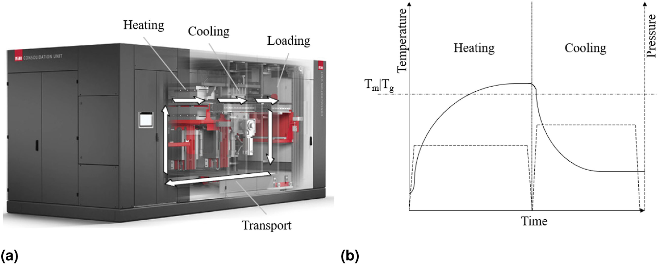

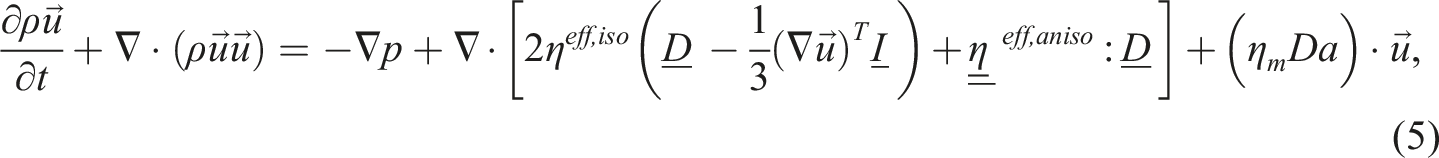
In order to simulate the flow behavior of the tape stack we adapted and numerically solved the anisotropic squeeze-flow model proposed by Rogers.⁸ The simulation was performed using the open-source Computational Fluid Dynamics (CFD) software OpenFOAM^®, where we extended a an existing solver to model the complex flow of a multi-region, multi-phase, and multi-component mixture that contains a molten matrix with fibers, all under non-isothermal and transient conditions.⁷

We have previously successfully confirmed the solver’s ability to predict squeeze flow in a laboratory-scale consolidation unit.⁹ The present work aimed to extend its application to an industrial-scale consolidation process, specifically focusing on predicting thickness and area of final parts.

Modeling

Governing equations

In order to predict the final geometric properties (i.e., thickness and area) of the semi-finished product after consolidation, we simulated the process at 13 different settings (see Table 1). For this purpose, a numerical solver described in Refs. 7 and 9 was used. Below, only the basic setup and the fundamental equations for modelling a transient, non-isothermal, incompressible, Newtonian fluid flow are described. The assumption that thermoplastic composites can be treated as an incompressible material is commonly applied.^10–17 Since the pressure is usually low during the heating cycle and the temperature drop during cooling is so rapid that no material flow is observed,¹⁸ the shear rates occurring within the material are generally low, which justifies the assumption of Newtonian behavior.

Table 1.

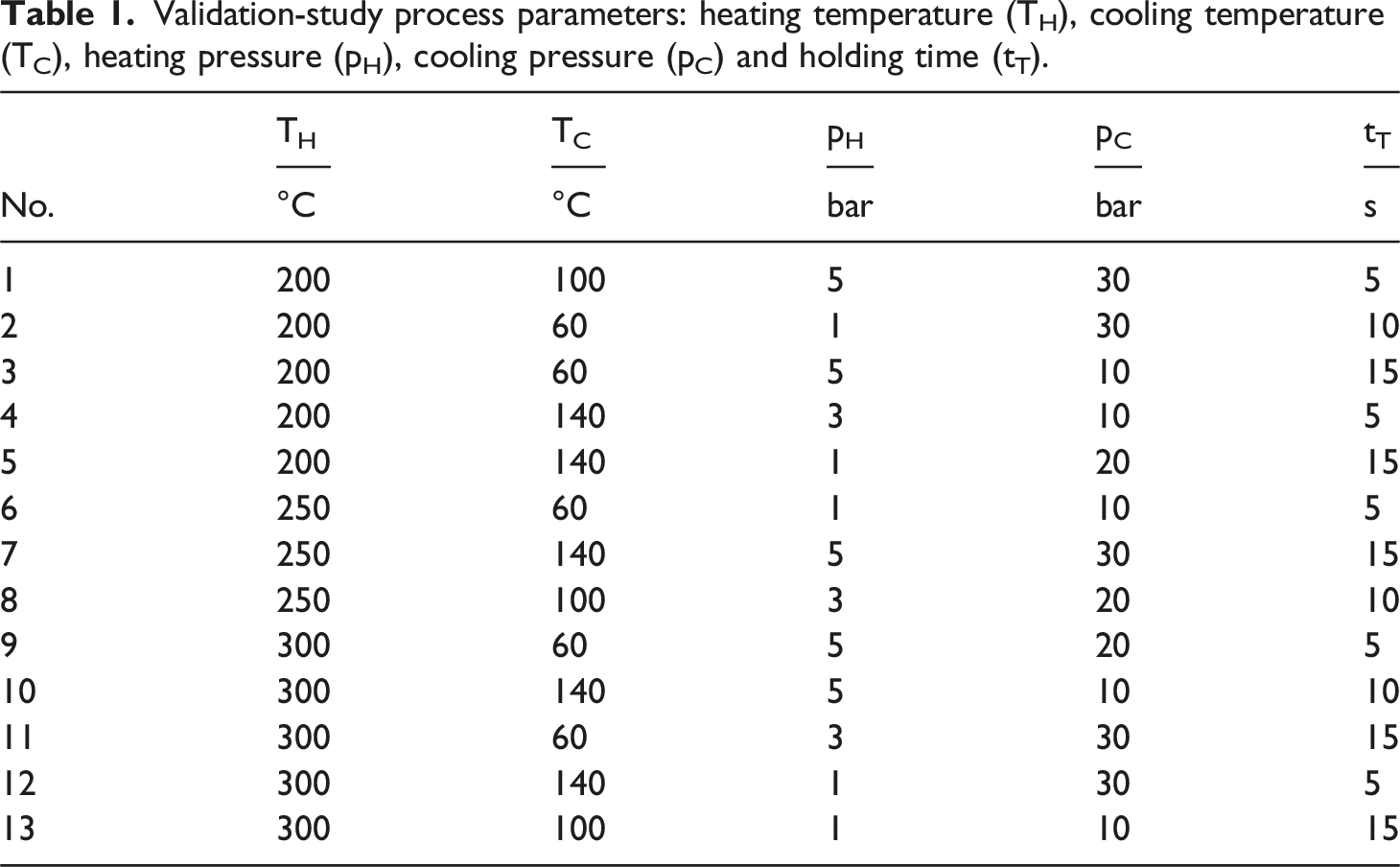
Validation-study process parameters: heating temperature (T_H), cooling temperature (T_C), heating pressure (p_H), cooling pressure (p_C) and holding time (t_T).

No.	T_H	T_C	p_H	p_C	t_T
No.	°C	°C	bar	bar	s
1	200	100	5	30	5
2	200	60	1	30	10
3	200	60	5	10	15
4	200	140	3	10	5
5	200	140	1	20	15
6	250	60	1	10	5
7	250	140	5	30	15
8	250	100	3	20	10
9	300	60	5	20	5
10	300	140	5	10	10
11	300	60	3	30	15
12	300	140	1	30	5
13	300	100	1	10	15

To reduce the complexity of the mathematical model, the composite material is treated as a homogeneous multi-component mixture whose thermodynamic behavior is described by linear mixing rules (see equation (7)). These empirical relationships provide macroscopic descriptions of the properties of the tape stack (e.g. heat conductivity, heat capacity) based on the properties of the fibers and the matrix. Rather than resolving the microscopic structure of the fiber-matrix-system, the approach approximates the behavior of the laminate on a macroscopic level. In particular, this entails that fiber-fiber interactions are ignored. The consolidated tapes are further assumed to be defect-free, i.e., local imperfections such as voids are omitted. In addition, the following assumptions and simplifications are made:

• Microscopic void dynamics are ignored.

• Considering the amorphous nature of the polycarbonate, crystallization kinetics are omitted.

• Degradation effects are ignored due to the sufficient thermal stability of the matrix material at common consolidation temperatures.

• The disparity between the coefficients of thermal expansion of the matrix and fiber has been ignored. The authors hypothesize that the influence of processing parameters (e.g., pressure), on the final dimensions of the component, is so pronounced, that the dimensional changes induced by the thermal expansion coefficients are inconsequential.

• Due to lack of reproducibility, idealized experimental boundary conditions are assumed. In particular, tool bending or inhomogeneous expansion of the tools and heating plates and associated residual stresses are ignored.

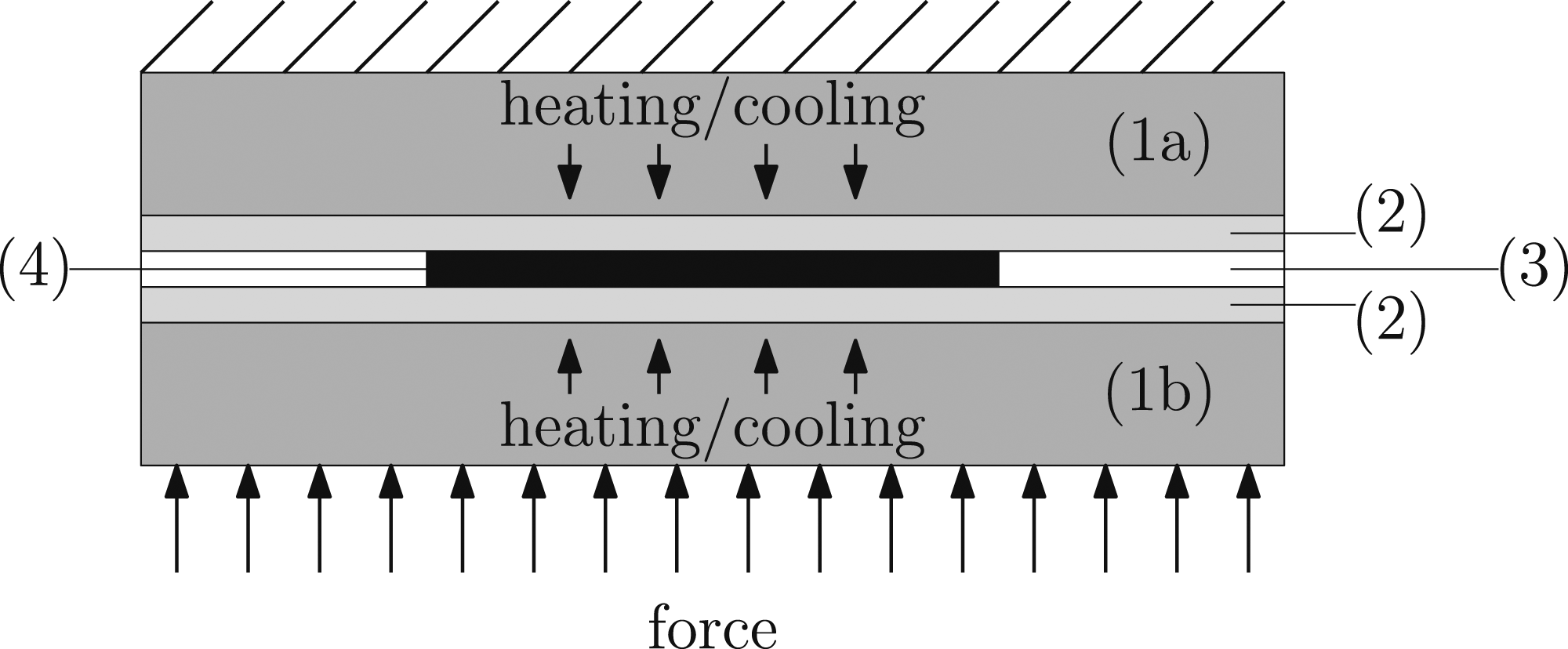
Within the model, the computational grid is divided into several solid domains (i.e., the heating/cooling plates and tools) and a fluid domain (see Figure 2).

Figure 2.

Illustration of the region of interest with the solid domains: heating/cooling plates (1a) and (1b) and tools (2); and the two phases of the fluid domain: air (3) (white indicates α = 0), and composite part (4) (black indicates α = 1).⁹

The solid domains are taken into account to model the heat transfer from the heating/cooling plates via the tools to the composite part and vice versa. Thus, only the energy conservation equation (1) based on pure heat conduction is solved

\frac{\partial ρ h}{\partial t} = \nabla \cdot (α_{t h} \nabla h),

(1)

where h is the specific enthalpy and α_th the thermal diffusivity. The latter is obtained from

α_{t h} = \frac{λ}{ρ \cdot c_{p}},

(2)

where λ is the heat conductivity, ρ is the density, and c_p is the specific heat capacity at constant pressure. Within the fluid region, two phases are considered: the composite part and its surrounding air. To describe the phase transport the Volume of Fluid (VOF) method is used

\frac{\partial α}{\partial t} + \nabla \cdot (\vec{u} α) + \nabla \cdot ({\vec{u}}_{r} α (1 - α)) = 0 .

(3)

In equation (3), α is a dimensionless parameter that describes the presence of a phase within a volume element;if a particular volume element contains composite, then α = 1; if it contains air, then α = 0 (see Figure 2). Smearing of the two immiscible phases (i.e., 0 < α < 1) is corrected by the last term on the left side of the equation, where ${\vec{u}}_{r}$ is directed against the fluid flow.¹⁹

To describe the flow in the fluid region of our model, the mass and momentum equations are written as

\nabla \cdot \vec{u} = 0;

(4)

\begin{matrix} \frac{\partial ρ \vec{u}}{\partial t} + \nabla \cdot (ρ \vec{u} \vec{u}) = - \nabla p + \nabla \cdot [2 η^{eff,iso} (\underset{̲}{D} - \frac{1}{3} {(\nabla \vec{u})}^{T} \underset{̲}{I}) + {\underset{̲}{\underset{̲}{η}}}^{eff,aniso} : \underset{̲}{D}] + (η_{m} \vec{D a}) \cdot \vec{u}, \end{matrix}

(5)

where

\vec{u}

is the velocity, p is the pressure, η^eff,iso is the effective isotropic viscosity,

{\underset{̲}{\underset{̲}{η}}}^{eff,aniso}

is the effective anisotropic viscosity,

\underset{̲}{D}

is the rate-of-deformation tensor, η_m is the viscosity of the matrix, and

\vec{D a}

is the Darcy coefficient, which describes a flow resistance. Equation (5) considers the anisotropic squeeze flow based on fiber orientation, assuming that the fibers are rigid and therefore do not change their orientation.

Typically, the computational mesh is structured to have one tape layer within each cell in the thickness direction, which allowes a tape stack with various fiber orientations to be represented. However, as the composite is regarded as a bulk material, no interface effects between individual tape layers are considered, and thus no specific boundary conditions are enforced at the interfaces between individual layers (i.e., ply-ply friction is omitted).

Detailed information about the variables mentioned above, the treatment of the fourth-order tensor ${\underset{̲}{\underset{̲}{η}}}^{eff,aniso}$ and the calculation procedure that leads to equation (5) is given in Ref. 9.

To include nonisothermal effects, we additionally solve the energy equation of the form

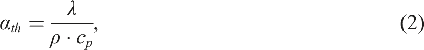
\frac{\partial ρ e}{\partial t} + \nabla \cdot ρ \vec{u} e - [\nabla \cdot \vec{u} p] + \frac{\partial ρ K}{\partial t} + \nabla \cdot ρ \vec{u} K = \nabla \cdot α_{t h, e f f} \nabla e,

(6)

The first three terms describe the variations in inner energy e over time, inner energy convection, and compression heating. The remaining terms on the left-hand side indicate the changes in mechanical energy K with time and mechanical energy convection. On the right-hand side, equation (6) accounts for heat conduction, where α_th,eff denotes the effective thermal diffusivity. The properties of the composite material, comprising both the matrix and fibers, such as density ρ_M, thermal conductivity λ_M, and specific heat capacity c_(p,M), are determined by applying the rule of mixture (equation (7))²⁰

(\begin{matrix} ρ_{M} \\ λ_{M} \\ c_{p, M} \end{matrix}) = Φ (\begin{matrix} ρ_{m} \\ λ_{m} \\ c_{p, m} \end{matrix}) + (1 - Φ) (\begin{matrix} ρ_{f} \\ λ_{f} \\ c_{p, f} . \end{matrix}),

(7)

where Φ is the fiber volume fraction and the subscript M corresponds to the matrix-fiber mixture, while subscripts m and f denote the matrix/fiber, respectively.

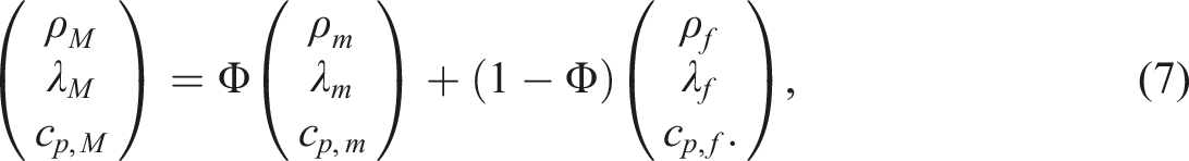
The density ρ_m and the specific heat capacity c_p,m of the matrix were measured at several temperatures using a high capillary rheometer (HKR Rheograph 25, GÖTTFERT Werkstoff-Prüfmaschinen GmbH, Buchen, Germany) and differential scanning calorimetry using a Mettler Toledo DSC 1 (Mettler Toledo Group, Columbus, OH, USA), respectively. From these data a polynomial fit was generated. The properties of the fibers ρ_f, λ_f, and c_p,f were evaluated using literature values.

More details on how the material data and associated boundary conditions that influence the thermodynamic response were obtained can be found in Ref. 7.

Initial and boundary conditions

During consolidation a force or pressure is applied to the composite part. To simulate the flow response caused by the pressure p(t) exerted on the part, a boundary condition is incorporated to compute p(t) from the applied force magnitude 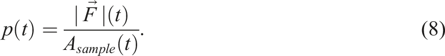$| \vec{F} | (t)$ acting on a projected sample area A_sample(t).

p (t) = \frac{| \vec{\vec{F}} | (t)}{A_{sample} (t)} .

(8)

As the sample undergoes compression, its projected area A_sample(t) changes with time, and the computed pressure p(t) adjusts accordingly. In practice, the applied pressure or force varies during an experiment due to the motion of the heating/cooling plates’ pistons. To account for this, the boundary condition retrieves force data from a table with corresponding time values obtained from the experiments.

Additionally, a slip boundary condition is set at the interfaces between the part and the tools, reflecting application of a release agent in the experiments that prevents the composite part from adhering to the tool. At the interface where the pressure acts on the part, the boundary condition calculates the mean velocity based on the pressure, using the flux φ(t)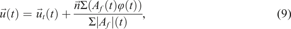

\vec{u} (t) = {\vec{u}}_{t} (t) + \frac{\vec{n} Σ (A_{f} (t) φ (t))}{Σ | A_{f} | (t)},

(9)

where

{\vec{u}}_{t} (t)

is the tangential velocity component, which represents the friction-free slip condition. Here,

\vec{n}

denotes the normal vector of the interface, A_f(t) the area of each cell face at the boundary, and |A_f|(t) the magnitude of the face areas.

To model the compression of the part due to the applied pressure, a boundary condition for cell displacement $(\vec{d} (t))$ is introduced. This condition computes the integral of the interface velocity ${\vec{u}}_{i} (t)$ over time

\vec{d} (t) = \int_{t - 1}^{t} {\vec{u}}_{i} (t) d t .

(10)

To simulate the heat transfer between the heating/cooling plates, tools, and the composite material, a boundary condition for heat conduction is employed. To this end, a value fraction vf is computed at the interface of two regions (i.e., solid/solid or solid/fluid). This fraction is then used to determine the wall temperature T_w

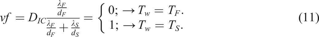
v f = D_{I C} \frac{\frac{λ_{F}}{d_{F}}}{\frac{λ_{F}}{d_{F}} + \frac{λ_{S}}{d_{S}}} = \{\begin{matrix} 0; \to T_{w} = T_{F} . \\ 1; \to T_{w} = T_{S} . \end{matrix}

(11)

The subscripts F and S pertain to the fluid and solid regions, respectively, while d characterizes the thickness of a finite volume element at the corresponding boundary wall. To account for heat transfer being impeded by surface roughness, equation (11) introduces the degree of intimate contact D_IC

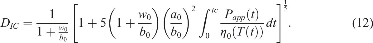
D_{I C} = \frac{1}{1 + \frac{w_{0}}{b_{0}}} {[1 + 5 (1 + \frac{w_{0}}{b_{0}}) {(\frac{a_{0}}{b_{0}})}^{2} \int_{0}^{t c} \frac{P_{app} (t)}{η_{0} (T (t))} d t]}^{\frac{1}{5}} .

(12)

This concept is grounded in the assumption that, due to surface roughness, contact is not immediately perfect, as detailed in Ref. 21. The degree of contact provides a simplified representation of the surface roughness, which is assumed to be approximately rectangular in shape. It is defined by the initial geometric parameters, this is, the distance between two rectangles w₀, the width b₀ and height a₀ of a rectangle, as well as the applied pressure P_app, and the temperature dependent dynamic zero viscosity η₀(T), as discussed in Refs. 22, 5 and 23.

In cases in which ideal contact between the heating/cooling plates and the tools, which would facilitate efficient heat conduction, is not achievable, a thin layer of air is taken into account in the boundary condition. This results in the following equation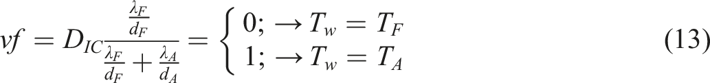

v f = D_{I C} \frac{\frac{λ_{F}}{d_{F}}}{\frac{λ_{F}}{d_{F}} + \frac{λ_{A}}{d_{A}}} = \{\begin{matrix} 0; \to T_{w} = T_{F} \\ 1; \to T_{w} = T_{A} \end{matrix}

(13)

where the index A refers to the air layer.

To model the transition from heating to cooling, the temparture of the press (see 1a and 1b in Figure 2) and the applied pressure are adapted accordingly.

Solution procedure

Figure 3 illustrates the sequence in which the previously explained equations are solved.

Figure 3.

Solution procedure for simulating the consolidation process.⁹

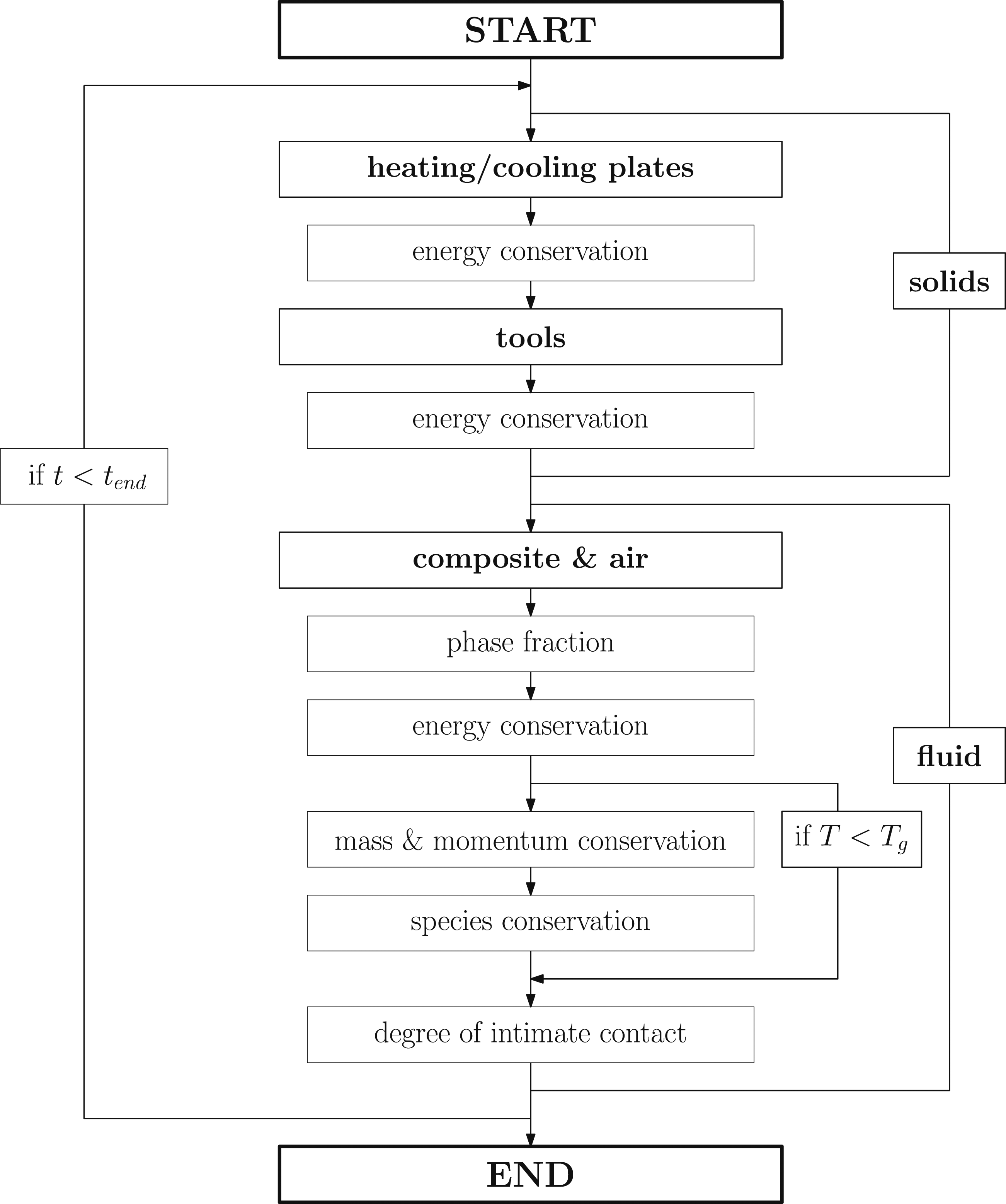
Our simulation procedure involves the following steps: First, the energy conservation equation (1) is solved specifically for the solid components (i.e., the heating/cooling plates and tools) to ensure that heat transfer within and between these solid parts is accurately accounted for. A set of equations (3)–(6) that pertain to the fluid phases (i.e., air and the composite material) is then solved, to model the fluid flow as well as the heat transfer within the fluid and between fluid and solids, respectively. The anisotropic squeeze flow, as previously described, is then computed. This calculation is integrated within the mass and momentum conservation equations, which allows the flow behavior resulting from the applied pressure and other relevant factors to be represented. Note that this work focused primarily on anisotropic squeeze flow, and consequently the description of species conservation, as indicated in Figure 3, was intentionally excluded.

To prevent numerical instabilities and for the sake of simplification, a threshold to the composite temperature is established: When the composite’s temperature is below the user-defined threshold (i.e., the glass-transition temperature T_g), the calculations for mass and momentum conservation are bypassed, as the material is assumed to be in a solid state.

Experimental

We validated our model at industrial scale with experimental data presented in Ref. 24. For these consolidation experiments, we used Maezio CF GP 1003T UD tapes composed of polycarbonate with carbon fiber (PC/CF) with an approximate fiber volume content of 44% as per the material supplier’s data sheet. To assemble the tape stacks, we employed a tape-laying cell based on the pick-and-place principle.⁶ Each stack consisted of 12 layers of UD tapes arranged in the sequence [0°/90°/0°/90°/0°/90°]_S. The nominal dimensions of the tape stack were 230 × 150 × 2.1 mm. The tape stacks were consolidated using a FILL SM-03 consolidation unit, as illustrated in Figure 1(a). Details on the consolidation process used in this work are given in Ref. 24.

The experiments were conducted using a definitive screening design, that comprised 13 distinct settings, which in the context of validation represents a wide range of settings. An overview of this experimental design is provided in Table 1. The holding time (t_T) is an additional time period for which the part is kept in the heating press beyond that necessary for the core of the part to reach the set temperature. This parameter was established based on insights obtained from preliminary tests.²⁴ Each consolidation parameter setting resulted in the production of 12 plates; note, that no flow restrictions were imposed on the tape stack during consolidation.

To determine the dimensional changes of the composite parts after consolidation, we measured area and thickness of the specimens. For capturing the area of the plates, we used a high-resolution 64-megapixel camera. Since some of the specimens showed distortion a 500 × 500 × 6 mm anti-reflective white glass was placed on them, which helped to flatten the samples. This glass was essential for reducing distortions and ensuring precise area measurements. Figure 4 shows a schematic representation of the setup used. The thickness of the consolidated plates was determined using a micrometer with a precision of ± 0.01 mm. Further details about the measurement process are provided in Ref. 24.

Figure 4.

Schematic drawing of the experimental setup of the area measurement. Adapted from Ref. 24.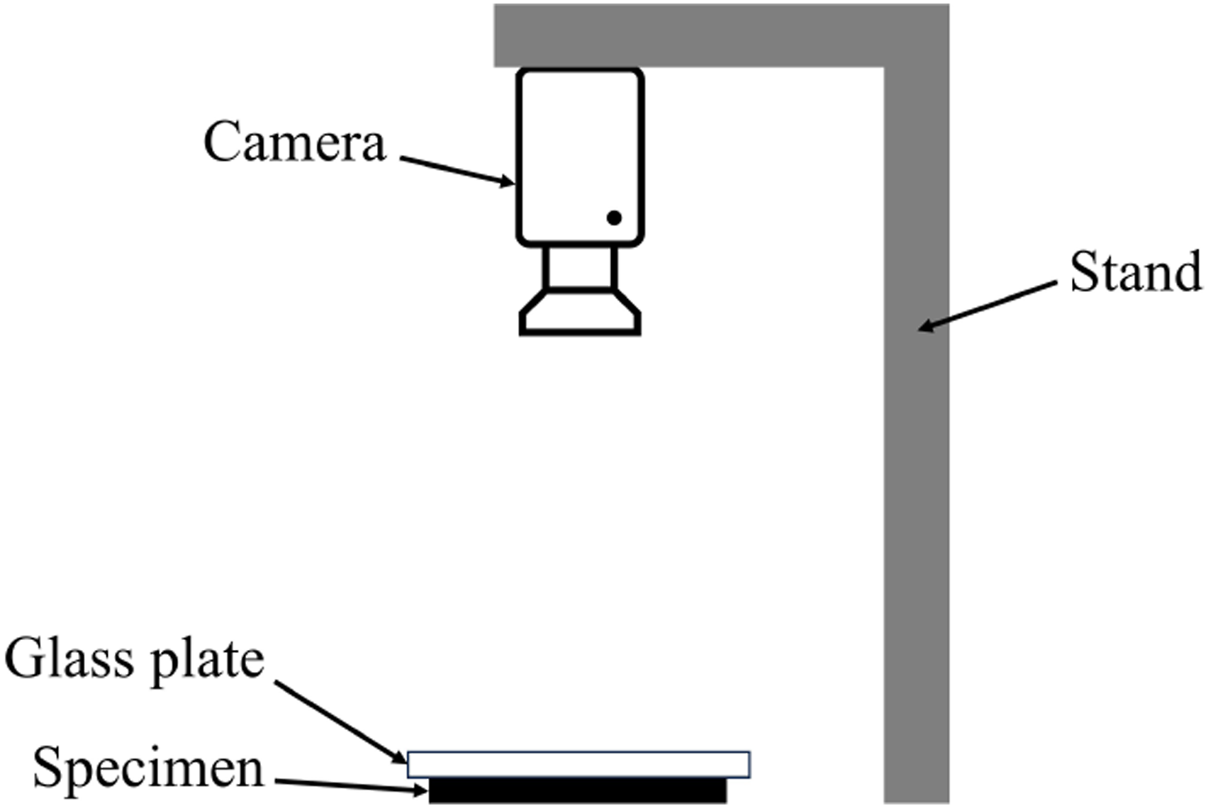

Results and Discussion

Since this work focused primarily on the validation of the model, the discussion of experimental results is omitted. Readers interested in the experimental findings are referred to our prior publication.²⁴

To ensure that the thermodynamic behavior of the process was correctly modeled, we compared our results with thermocouple data recorded at various positions within the tape layup. The results of this study were presented in Ref. 7.

Figure 5 compares the experimental and simulated results for area and thickness changes after consolidation, the indicators of squeeze flow.

Figure 5.

Comparison between experiment and simulation in terms of (a) thickness change and (b) area change.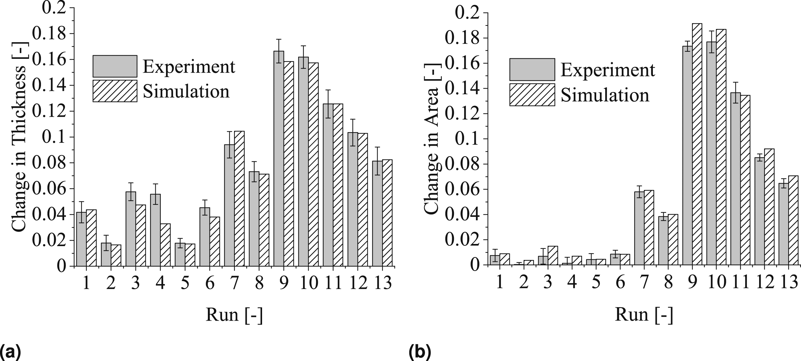

As shown in Figure 5, the overall difference between simulation and experimental data is small. However, note that for certain cases, the simulation results exhibited more pronounced deviations from the corresponding experimental data. For a more detailed analysis, Figures 6 and 7 show the thickness and area changes based on the specific parameter settings employed in the experimental study.

Figure 6.

Comparison between experiment and simulation in terms of thickness change based on the process parameters (A) holding time, (B) cooling pressure, (C) cooling temperature, (D) heating pressure, and (E) heating temperature.

Figure 7.

Comparison between experiment and simulation in terms of area change based on the process parameters (A) holding time, (B) cooling pressure, (C) cooling temperature, (D) heating pressure, and (E) heating temperature.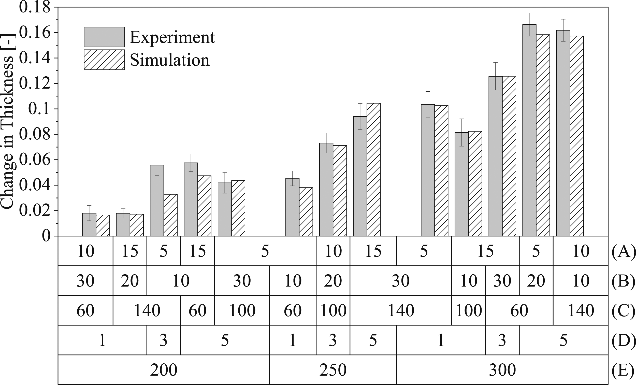

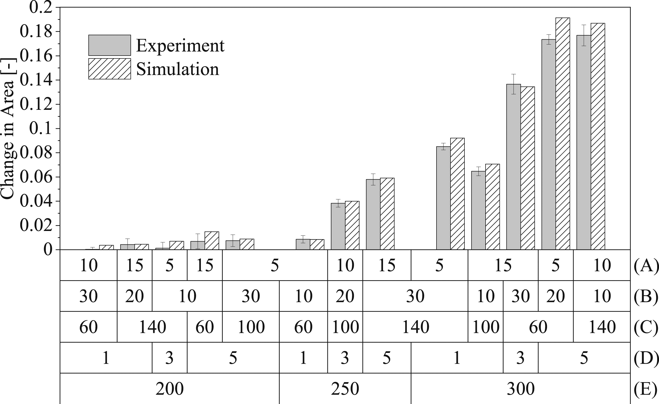
Figures 6 and 7 illustrate the primary factors influencing squeeze flow: heating temperature (E), heating pressure (D) and, to a lesser extent, cooling temperature (C). The cooling pressure exhibited minimal impact on part dimensions. This can be attributed to the rapid temperature decrease upon exposure to the cooling press resulting in increased viscosity and, consequently, constrained flow.^7,24 It is noticeable that the majority of the simulation results fall within the standard deviation of the experiments, except for the cases with a heating temperature of 200°C.

Figure 8 compares simulation and experiment in terms of the changes in thickness and area of the parts consolidated at 200°C heating temperature. Due to the assumption of an incompressible material in the simulation a certain relationship is evident between changes in thickness and in area. This behavior, however, was rare in the experiments because the high viscosity at such low heating temperatures does not allow the material to flow. Instead, a compaction is observed caused by softening of the matrix due to heat and alignment of the layers. This effect is not accurately represented in the simulation.

Figure 8.

Comparison between experiment and simulation in terms of thickness and area change.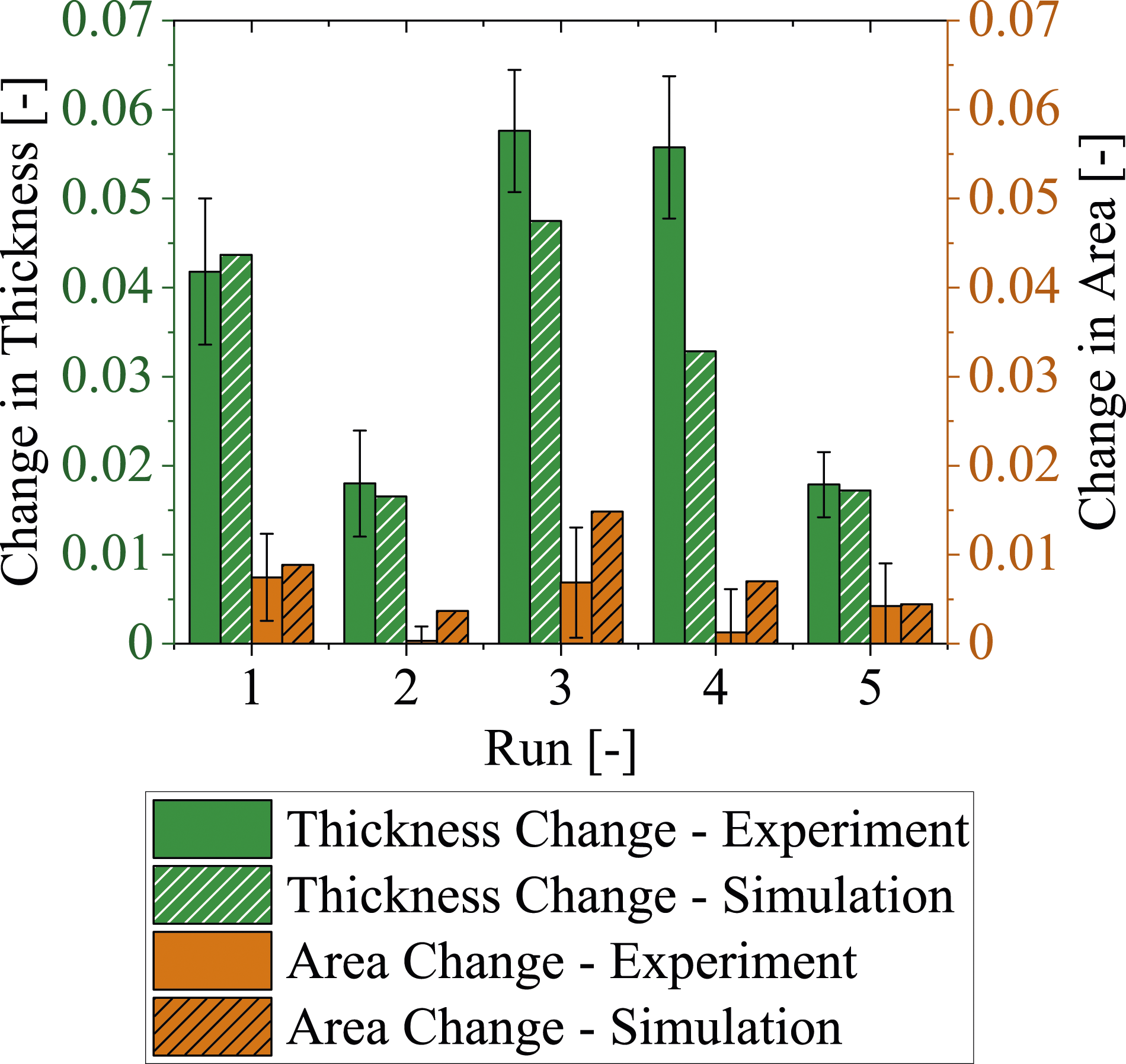

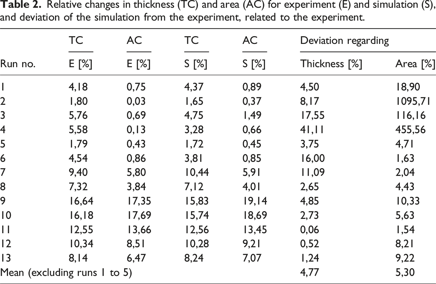
Table 2 summarizes the deviations of the simulation from the experiment in terms of changes in thickness and area. It can be seen that for runs 1–5 the deviations are considerable, especially regarding the area change. The reason for this, as explained above, is that in the experiments at this low heating temperature (200°C) no flow, but compaction is observed, which is not modeled in the simulation. The absolute mean deviations for runs 6–13, however, are satisfactory at 4.77% and 5,30% for the thickness and area changes, respectively.

Table 2.

Relative changes in thickness (TC) and area (AC) for experiment (E) and simulation (S), and deviation of the simulation from the experiment, related to the experiment.

Run no.	TC	AC	TC	AC	Deviation regarding
Run no.	E [%]	E [%]	S [%]	S [%]	Thickness [%]	Area [%]
1	4,18	0,75	4,37	0,89	4,50	18,90
2	1,80	0,03	1,65	0,37	8,17	1095,71
3	5,76	0,69	4,75	1,49	17,55	116,16
4	5,58	0,13	3,28	0,66	41,11	455,56
5	1,79	0,43	1,72	0,45	3,75	4,71
6	4,54	0,86	3,81	0,85	16,00	1,63
7	9,40	5,80	10,44	5,91	11,09	2,04
8	7,32	3,84	7,12	4,01	2,65	4,43
9	16,64	17,35	15,83	19,14	4,85	10,33
10	16,18	17,69	15,74	18,69	2,73	5,63
11	12,55	13,66	12,56	13,45	0,06	1,54
12	10,34	8,51	10,28	9,21	0,52	8,21
13	8,14	6,47	8,24	7,07	1,24	9,22
Mean (excluding runs 1 to 5)					4,77	5,30

The alignments between changes in thickness and area in experiment and simulation are shown in the scatter plots shown in Figure 9 for all 13 cases. As can be seen, with a few notable exceptions, predictions agree well with the experimental data, which indicates a generally accurate fit.

Figure 9.

Scatter plots of the thickness (a) and area (b) changes - experiment versus simulation.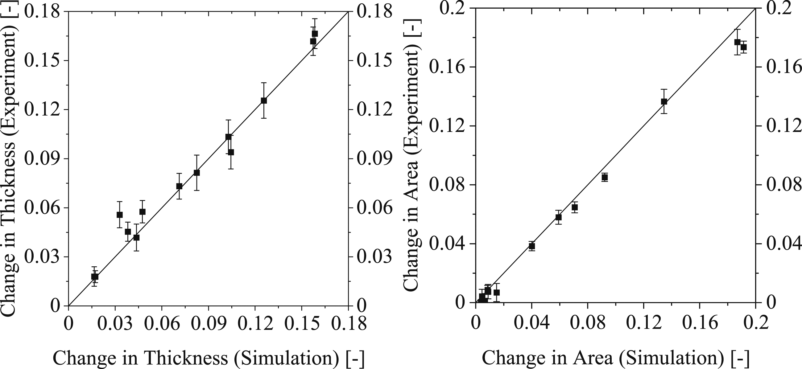

Figure 10 presents the qualitative comparison between simulation run No. 10 and a corresponding specimen obtained by experiment.

Figure 10.

Qualitative comparison between experiment (a) and simulation (b) for run No. 10, with length and width in meters.¹⁸

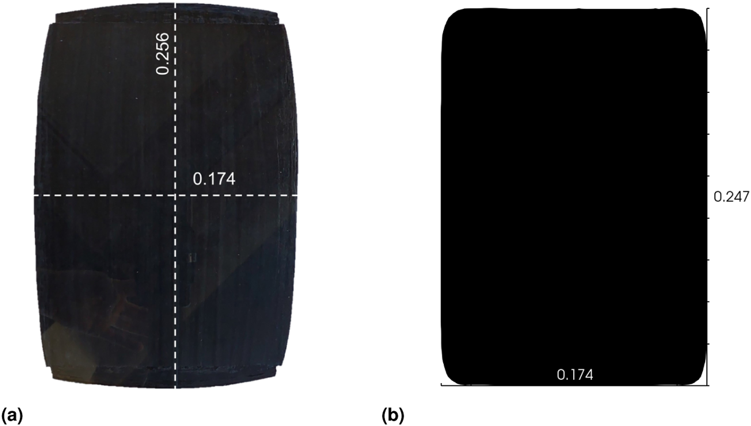
It is evident that the relative slipping of individual tapes, which is not accurately modeled by the simulation, leads to differences in the qualitative comparison, especially at the corners of the composite part. Further, the edges of the specimen are slightly bent, with the fibers appearing curved. Since the simulation does not account for changes in fiber direction, it fails to model these effects. As illustrated in Figure 10(b), contrary to the experimental observations, the edges in the simulation are nearly straight.

Conclusion

In this study, we expanded the applicability of our consolidation model for anisotropic squeeze flow from laboratory-scale experiments to an industrial-scale process. Our primary objective was to validate the reliability of our predictions by assessing changes in both the area and the thickness of composite parts after consolidation.

Anisotropic squeeze flow plays a key role in determining the geometric characteristics of semi-finished products, as it can induce significant alterations in part thickness and area. In practical applications it is crucial to avoid excessive squeezing, as experiments have shown that it can give rise to internal stresses and deformations, and to marked dimensional changes that may cause the part to no longer meet design and application specifications. Our approach allows the squeeze flow to be estimated as a function of process settings, thus avoiding time-, material- and energy-consuming experiments.

From Figures 6 and 7 it can be seen that the parameters with greater influence are the heating temperature (E) and the heating pressure (D), which is evident in both experiment and simulation.

In both the experimental and the simulation data, the change in area does not correspond directly to change in thickness in cases involving lower heating temperatures, specifically at 200°C. In the experimental context, this observation can be attributed to the compaction behavior of individual tape layers, which, due to relatively high matrix viscosity at lower temperatures, results in a limited change in area. Since this phenomenon is not accurately modeled in the simulation, as the material is assumed to be incompressible, this leads to relatively large deviations of the simulation from the experiment in terms of thickness and especially area change.

In the simulation, the tape layup is treated as a bulk material, and any significant change in thickness naturally induces alterations in both width and length. The extent of thickness change required to trigger an area change depends on the mesh resolution. In particular, if the resolution is too coarse, it can lead to inaccuracies in modeling the phase transport. Taking this into consideration allows fine-tuning of the simulation by adjustment of the mesh resolution to better align with the experimental data.

The mean deviation of the simulation from the experimental data in terms of thickness change was 8.7%. When the runs involving a heating temperature of 200°C are excluded, the mean deviation in area change decreases to 5.3%.

The qualitative comparison, consistent with the findings given in Ref. 9, emphasizes that the omitting consideration of changes in fiber orientation caused by squeeze flow leads to inadequate representation of curved-edge formation. Furthermore, treating the composites as a bulk material ignores relative slippage of individual tapes and introduces qualitative discrepancies between simulation and experimental results, which are particularly pronounced at the corners of the part.

As mentioned in our prior publication,⁹ further investigations are required to (i) validate the assumption of an incompressible material by accounting for possible voids within the tape material,^25,26 (ii) include a model, which accounts for the bonding quality after consolidation, (iii) consider changes in fiber orientation due to squeeze flow and their effects on part geometry, (iv) examine crystallization effects in semi-crystalline materials, and (v) optimize simulation time, potentially by implementation of symmetry conditions and further simplifications.

Furthermore, the impact of flow restriction, for instance by use of a frame, should be explored in the simulation and subsequently compared with experimental results.

Footnotes

Acknowledgments

The authors acknowledge financial support by the COMET Centre CHASE, which is funded within the framework of COMET—Competence Centers for Excellent Technologies—by BMVIT, BMDW, and the Federal Provinces of Upper Austria and Vienna. The COMET program is run by the Austrian Research Promotion Agency (FFG).

Declaration of conflicting interests

The author(s) declared no potential conflicts of interest with respect to the research, authorship, and/or publication of this article.

Funding

The author(s) disclosed receipt of the following financial support for the research, authorship and/or publication of this article: This work was performed within the Competence Center CHASE GmbH, funded by the Austrian Research and Promotion Agency.

ORCID iDs

Eva Kobler

Christian Marschik

Data availability statement

The data presented in this study are available on request from the corresponding author.*

Symbols

References

IMARC . Thermoplastic composites market: global industry trends, share, size, growth, opportunity and forecast 2023-2028. https://www.imarcgroup.com/thermoplastic-composites-market

Gardiner

. Thermoplastic composites gain leading edge on the a380. High Perform Compos 2006; 14: 50–55.

Slange

. Rapid manufacturing of tailored thermoplastic composites by automated lay-up and stamp forming - a study on the consolidation mechanisms. Twente: University of Twente, 2019.

Slange

Warnet

Grouve

, et al. Influence of preconsolidation on consolidation quality after stamp forming of c/peek composites. In: Proceedings of the 19th International ESAFORM Conference on Material Forming, Nantes, France, 27-29 April 2016.

Mantell

Wang

Springer

. Processing thermoplastic composites in a press and by tape laying - experimental results. J Compos Mater 1992; 26: 16.

Birtha

Marschik

Kobler

, et al. Optimizing the process of spot welding of polycarbonate-matrix-based unidirectional (ud) thermoplastic composite tapes. Polymers 2023; 15(9): 2182. DOI: 10.3390/polym15092182.

Kobler

Birtha

Marschik

, et al. A novel multi-region, multi-phase, multi-component-mixture modeling approach to predicting the thermodynamic behaviour of thermoplastic composites during the consolidation process. Polymers 2022; 14: 4785, DOI: 10.3390/polym14214785.

Rogers

. Rheological characterization of anisotropic materials. Composites 1989; 20(1): 21–27.

Kobler

Birtha

Marschik

, et al. Modeling the anisotropic squeeze flow during hot press consolidation of thermoplastic unidirectional fiber-reinforced tapes. J Thermoplast Compos Mater 2023. DOI: 10.1177/08927057231214458.

10.

O’Brádaigh

Pipes

Mallon

. Issues in diaphragm forming of continuous fiber reinforced thermoplastic composites. Polym Compos 1991; 12(4): 246–256.

11.

Balasubramanyam

Jones

Wheeler

. Modelling transverse flows of reinforced thermoplastic materials. Composites 1989; 20: 33–37.

12.

Rogers

. Squeezing flow of fibre-reinforced viscous fluids. J Eng Math 1989; 23: 81–89.

13.

Christensen

. Effective viscous flow properties for fiber suspensions under concentrated conditions. J Rheol 1993; 37: 103–121.

14.

Shuler

Advani

. Transverse squeeze flow of concentrated aligned fibers in viscous fluids. J Non-Newtonian Fluid Mech 1996; 65: 47–74.

15.

Ericsson

Manson

. The two-way interaction between anisotropic flow and fiber orientation in squeeze flow. J Rheol 1997; 41(3): 493–511. DOI: 10.1122/1.550833.

16.

Goshawk

Navez

Jones

. Squeezing flow of continuous fibre-reinforced composites. J Non-Newtonian Fluid Mech 1997; 73: 327–342.

17.

Loredo

Klöcker

. Generalized inverse of the compliance tensor, and behaviour of incompressible anisotropic materials - application to damage. Mech Res Commun 1997; 24(4): 371–376.

18.

Kobler

. Modeling the consolidation process of thermoplastic UD tapes. doctoralthesis. Linz: Johannes Kepler Universität, 2023.

19.

Weller

. A new approach to vof-based interface capturing methods for incompressible and compressible flow. Technical Report Report TR/HGW 4. OpenCFD Ltd., 2008.

20.

Lee

Jeong

Choi

, et al. Composite materials. Seoul, Korea: Hongrung Publishing Company, 2007.

21.

Loos

Dara

. Processing of thermoplastic matrix composites. In: Review of progress in quantitative nondestructive evaluation. New York: Springer, 1987, pp. 1257–1265.

22.

Levy

Heider

Tierney

, et al. Inter-layer thermal contact resistance evolution with the degree of intimate contact in the processing of thermoplastic composite laminates. J Compos Mater 2014; 48(4): 491–503. DOI: 10.1177/0021998313476318.

23.

Mantell

Springer

. Manufacturing process models for thermoplastic composites. J Compos Mater 1992; 26(16): 2348–2377. DOI: 10.1177/002199839202601602.

24.

Birtha

Kobler

Marschik

, et al. Using heating and cooling presses in combination to optimize the consolidation process of polycarbonate-based unidirectional thermoplastic composite tapes. Polymers 2023; 15(23): 4500. DOI: 10.3390/polym15234500.

25.

Tierney

Gillespie

Jr . Modeling of heat transfer and void dynamics for the thermoplastic composite tow-placement process. J Compos Mater 2003; 37(19): 1745–1768. DOI: 10.1177/002199803035188.

26.

Tierney

Gillespie

Jr . Modeling of in situ strength development for the thermoplastic composite tow placement process. J Compos Mater 2006; 40(16): 1487–1506. DOI: 10.1177/0021998306060162.

No.	T_H	T_C	p_H	p_C	t_T
No.	°C	°C	bar	bar	s
1	200	100	5	30	5
2	200	60	1	30	10
3	200	60	5	10	15
4	200	140	3	10	5
5	200	140	1	20	15
6	250	60	1	10	5
7	250	140	5	30	15
8	250	100	3	20	10
9	300	60	5	20	5
10	300	140	5	10	10
11	300	60	3	30	15
12	300	140	1	30	5
13	300	100	1	10	15

No.	T_H	T_C	p_H	p_C	t_T
No.	°C	°C	bar	bar	s
1	200	100	5	30	5
2	200	60	1	30	10
3	200	60	5	10	15
4	200	140	3	10	5
5	200	140	1	20	15
6	250	60	1	10	5
7	250	140	5	30	15
8	250	100	3	20	10
9	300	60	5	20	5
10	300	140	5	10	10
11	300	60	3	30	15
12	300	140	1	30	5
13	300	100	1	10	15

An experimental validation study of a numerical modeling approach to predicting post-consolidation dimensions of thermoplastic composites

Abstract

Keywords

Introduction

Modeling

Governing equations

Initial and boundary conditions

Solution procedure

Experimental

Results and Discussion

Conclusion

Footnotes

Acknowledgments

Declaration of conflicting interests

Funding

ORCID iDs

Data availability statement

Symbols

References

No.	T_H	T_C	p_H	p_C	t_T
No.	°C	°C	bar	bar	s
1	200	100	5	30	5
2	200	60	1	30	10
3	200	60	5	10	15
4	200	140	3	10	5
5	200	140	1	20	15
6	250	60	1	10	5
7	250	140	5	30	15
8	250	100	3	20	10
9	300	60	5	20	5
10	300	140	5	10	10
11	300	60	3	30	15
12	300	140	1	30	5
13	300	100	1	10	15