Modeling the anisotropic squeeze flow during hot press consolidation of thermoplastic unidirectional fiber-reinforced tapes

Abstract

The anisotropic material behavior of continuous-fiber-reinforced composites that is evident in their mechanical properties should also be considered in their processing. An important step in the processing of thermoplastic unidirectional (UD) fiber-reinforced tapes is consolidation, where a layup consisting of locally welded UD tape layers is firmly bonded. Compression of the molten thermoplastic matrix material during consolidation leads to a squeeze flow, the direction of which is determined by the fibers. This work presents a model that describes the influence of fiber direction on compression and flow behavior, implemented in the computational fluid dynamics (CFD) software tool OpenFOAM^®. To validate the simulation results, we performed experiments in a laboratory consolidation unit, capturing the squeeze flow with cameras and then quantifying it by gray-scale analysis. The specimens used were UD polycarbonate tapes (44% carbon fibers by volume) of various sizes and with various fiber directions. The simulation allows prediction of the changes in specimen geometry during consolidation and is a first step towards optimizing the process by avoiding extensive squeeze flow.

Introduction

Thermoplastic composites have become increasingly important in recent years: According to the International Market Analysis Research and Consulting (IMARC) Group, ¹ the annual growth rate of thermoplastic composites predicted for 2023-2028 is 6% and will reach a value of US $ 24.6 billion in 2028. Use of thermoplastic composites in aircrafts, such as the Airbus A380, is state of the art, and further applications in aerospace engineering are expected. ² These applications require the production of defect-free parts and thus highly controllable and reproducible processing techniques, in the context of which predicting part quality by simulation plays an essential role.

The processing of thermoplastic unidirectional (UD) continuous-fiber-reinforced tapes relevant to this work consists of the following steps: Tape laying, consolidation, preheating, and forming and functionalization, as shown in Figure 1.

Figure 1.

Processing of thermoplastic UD tapes: laying, consolidation, preheating and forming and functionalization.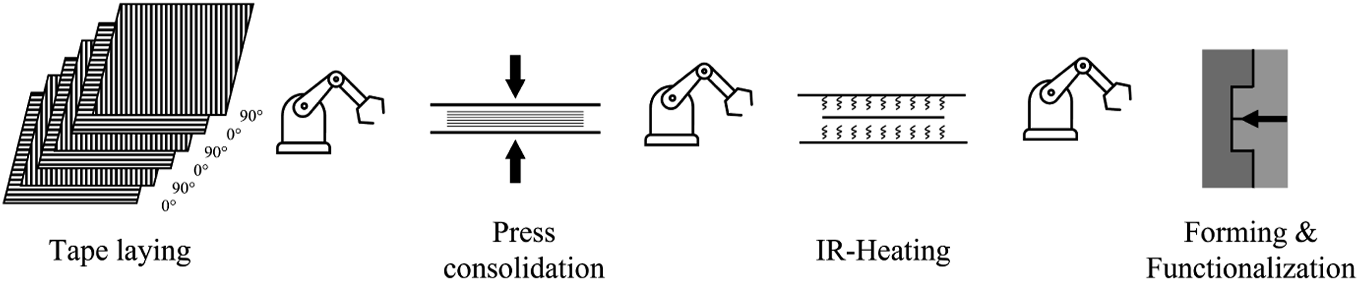

Since UD tapes can bear heavy loads only in the fiber direction, fiber orientations are often varied at the point of tape laying, e.g: in aerospace applications, the quasi-isotropic layup ([0°|± 45°|90°]_S) is widely used. ³ Tape laying can be fully automated in three ways: pick-and-place, automated tape laying (ATL), and automated fiber placement (AFP).

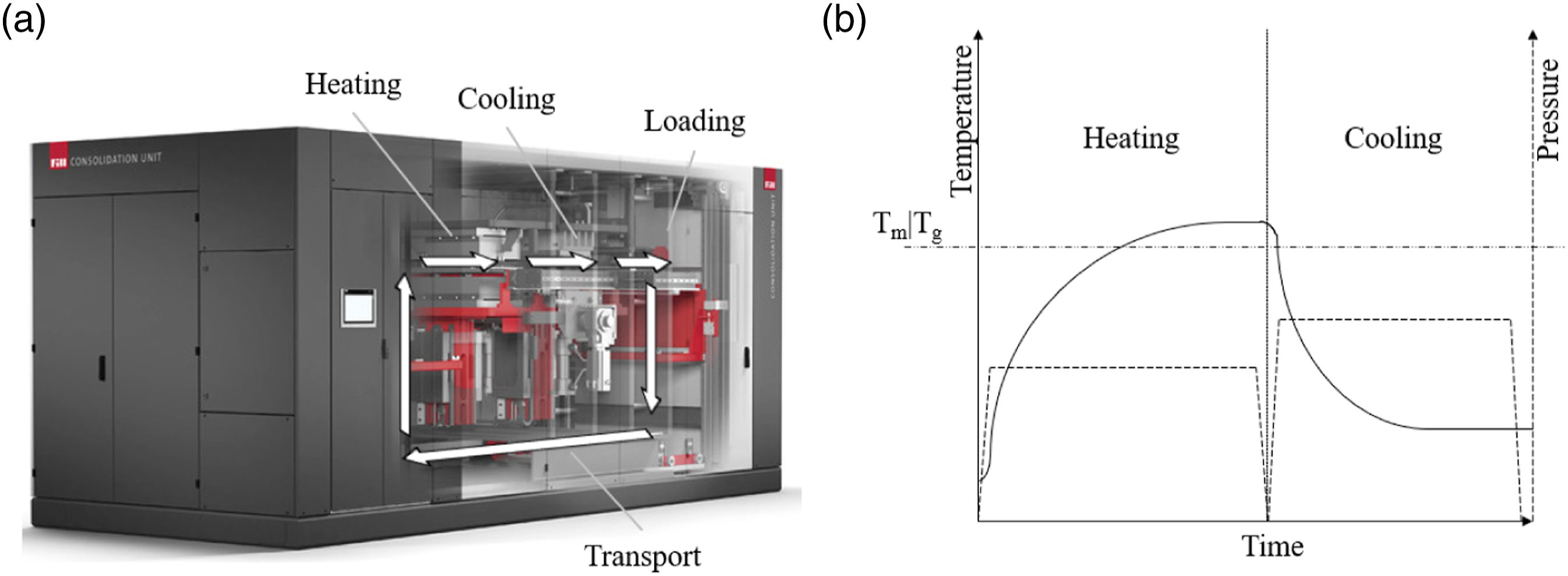
In the pick-and-place method, a robot places pre-cut tapes on top of each other and welds them locally using hot stamping ⁴ or ultrasonic welding. ⁵ This method requires subsequent consolidation. The consolidation process, on which this work concentrates, involves using hydraulic heating and cooling presses, where the layup is heated to a temperature higher than the glass-transition temperature (T _g ) for amorphous polymers or melting temperature (T _m ) for semi-crystalline polymers in a heating press and then cooled to a temperature below T _g or T _m in a cooling press (Figure 2). In both presses, consolidation of the layup takes place under pressure. In the next step, the consolidated stack is preheated, which involves heating the consolidated part above T _m for semi-crystalline polymers and above T _g for amorphous polymers to make it formable. This is usually done by infrared or convection ovens. ³ The forming process can be carried out in hydraulic presses or an injection molding machine, which can also be used for simultaneous overmolding and functionalization.

Figure 2.

(a) Consolidation unit used for composite processing on an industrial scale and (b) example temperature and pressure profiles during heating and cooling (adapted from ⁶ ).

In-situ consolidation during the ATL or AFP process can achieve sufficient consolidation quality without a seperate consolidation step. However, the bonding quality can be improved by hot press consolidation before preheating and forming, as this results in increased interlaminar shear strength (ILSS) and reduced porosity.^7–9

The well-known anisotropic behavior of continuous-fiber-reinforced composites clearly affects not only their mechanical properties, but also the processing of thermoplastic UD tapes, which has been discussed by numerous authors. The transverse isotropic flow approach, first described by Ericksen, ¹⁰ forms the basis for modeling the anisotropic squeeze flow, and has been developed further for various forms of processing, including injection molding of short- and long-fiber-reinforced polymers,^11–13 sheet-mold compounding,^14,15 and hot-press forming and consolidation.^16–21 This work builds on the approach by Rogers, ²² as it showed the highest numerical stability compared to other models.

To simulate the flow behavior of the tape stack (i.e., molten matrix including fibers) during the consolidation process with particular emphasis on the heating phase, the anisotropic squeeze-flow model by Rogers ²² was adapted and solved numerically using the open-source CFD (Computational Fluid Dynamics) software OpenFOAM^®. To this end, a solver developed in the course of previous work ⁶ was extended to model a multi-region, multi-phase and multi-component-mixture flow of an incompressible fluid under non-isothermal, transient conditions. To investigate the phenomenological basis of the anisotropic squeeze flow, experiments were carried out with a laboratory-scale consolidation unit. The data obtained were used to validate the developed model.

In the future, the simulation setup will be validated by experiments on an industrial plant.

Modeling

Governing equations

To predict the anisotropic flow behavior of a thermoplastic tape stack during the consolidation process, a fully three dimensional mathematical model described in detail in ⁶ was extended and then solved numerically in OpenFOAM^®.

Since the simulation approach is global and includes the composite, the heating and cooling plates, and the tools, the computational grid is split into solid and fluid domains, different assumptions are made and different equations are solved, respectively. For the solid domains (Figure 3), including the heating/cooling plates and the tools, the energy conservation equation (Equation (1)) is solved based on pure heat conduction:

$\frac{\partial \rho h}{\partial t}=\nabla ·\left({\alpha }_{th}\nabla h\right)$

(1)

where h is the specific enthalpy and α _th the thermal diffusivity, which is further defined by the heat conductivity λ, the density ρ, and the specific heat capacity at constant pressure c _p :

${\alpha }_{th}=\frac{\mathrm{\lambda }}{\rho ·c_p}.$

(2)

In the fluid area, the transport of the phases (composite and air) is generally described by the conservation equations of mass, momentum, and energy in combination with the Volume of Fluid (VOF) model (see Equations (3)–(5), and (21)). Since the computational mesh is chosen to model each layer by a volume cell through the thickness, it is possible to assign fiber directions and thus anisotropic properties to each layer. However, the composite is treated as a bulk material, i.e., no boundary conditions are imposed on the interface between individual layers.

$\frac{\partial \alpha }{\partial t}+\nabla ·\left(\overrightarrow{u}\alpha \right)+\nabla ·\left({\overrightarrow{u}}_r\alpha \left(1-\alpha \right)\right)=0,$

(3)

where α is a dimensionless parameter that indicates whether a cell contains composite (α = 1) or air (α = 0) (see Figure 3). The last term corrects for the smearing of the two immiscible phases (i.e., 0 < α < 1), with ${\overrightarrow{u}}_r$ directed against the fluid flow. ²³

Figure 3.

Illustration of the region of interest with the solid domains: heating/cooling plates (1a) and (1b) and tools (2); and the fluid domain: air (3) (white means α = 0), and composite part (4) (black means α = 1).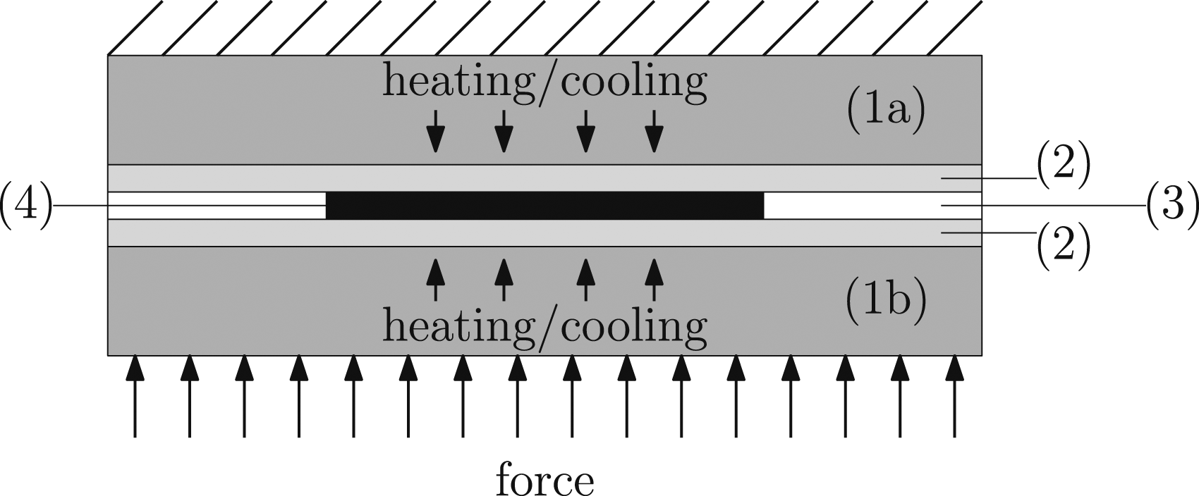

Mass and momentum conservation are described by:

$\nabla ·\overrightarrow{u}=0;$

(4)

$\frac{\partial \rho \overrightarrow{u}}{\partial t}+\nabla ·\left(\rho \overrightarrow{u}\overrightarrow{u}\right)={\overrightarrow{F}}_B+{\overrightarrow{F}}_S+{\overrightarrow{S}}_m,$

(5)

with $\overrightarrow{u}$ representing the velocity and ${\overrightarrow{F}}_S$ representing surface forces. Outer body forces ${\overrightarrow{F}}_B$ , such as gravity, are ignored within this work. ${\overrightarrow{S}}_m$ is an optional source or sink term, which is explained further below.

The original work of Rogers ²² uses the following equation to describe the anisotropic squeeze flow:

${\overrightarrow{F}}_S=\nabla ·{\underset{\_}{\sigma }}_F=\nabla ·\left[T_f\underset{\_}{a}-\overline{p}\underset{\_}{I}+\underset{\underset{\_}{\tau }}{\underset{ุ}{2{\eta }_T\underset{\_}{D}+2\left({\eta }_L-{\eta }_T\right)\left(\underset{\_}{a}·\underset{\_}{D}+\underset{\_}{D}·\underset{\_}{a}\right)}}\right],$

(6)

where T _f is an arbitrary fiber tension which represents the inextensibility of the fiber, $\underset{\_}{a}$ is the fiber orientation tensor, $\overline{p}$ is the hydrostatic pressure, $\underset{\_}{I}$ is the unity tensor, $\underset{\_}{\tau }$ is the viscous stress tensor, η _T and η _L are the transverse and longitudinal dynamic viscosity, and $\underset{\_}{D}$ is the rate-of-deformation tensor, which is further defined as:

$\underset{\_}{D}=\frac{1}{2}\left[\nabla \overrightarrow{u}+{\left(\nabla \overrightarrow{u}\right)}^T\right].$

(7)

In this work η _L and η _T are substituted by an anisotropic dynamic viscosity fourth-order tensor ${\underset{\_}{\underset{\_}{\eta }}}^{eff,aniso}$ and an isotropic dynamic viscosity fourth-order tensor ${\underset{\_}{\underset{\_}{\eta }}}^{eff,iso}$ , respectively. The sum of which gives the effective viscosity fourth-order tensor ${\underset{\_}{\underset{\_}{\eta }}}^{eff}$ shown by Wittemann ¹³ :

${\underset{\_}{\underset{\_}{\eta }}}^{eff}={\underset{\_}{\underset{\_}{\eta }}}^{eff,iso}+{\underset{\_}{\underset{\_}{\eta }}}^{eff,aniso}.$

(8)

The effective viscosity ${\underset{\_}{\underset{\_}{\eta }}}^{eff}$ is calculated by:

${\underset{\_}{\underset{\_}{\eta }}}^{eff}=\alpha ·{\underset{\_}{\underset{\_}{\eta }}}^{transverse}+\left(1-\alpha \right)·{\underset{\_}{\underset{\_}{\eta }}}^{air}.$

(9)

Applied to a cell containing only composite material (i.e., α = 1), the following applies:

${\underset{\_}{\underset{\_}{\eta }}}^{eff}={\underset{\_}{\underset{\_}{\eta }}}^{transverse},$

(10)

with the orientation averaged transverse viscosity $〈{\underset{\_}{\underset{\_}{\eta }}}^{transverse}〉$ calculated by:

$\begin{array}{l}〈{\underset{\_}{\underset{\_}{\eta }}}^{transverse}〉=\left({\eta }_{11}-4{\eta }_{12}+{\eta }_{23}\right)\underset{\_}{a}\otimes \underset{\_}{a}\\ +\left(-\frac{{\eta }_{11}}{3}+{\eta }_{23}\right)\left(\underset{\_}{a}\otimes \underset{\_}{I}+\underset{\_}{I}\otimes \underset{\_}{a}\right)\\ +\left({\eta }_{12}-{\eta }_{23}\right)\left(\underset{\_}{a}\square \underset{\_}{I}+\underset{\_}{I}\square \underset{\_}{a}+{\left(\underset{\_}{a}\square \underset{\_}{I}\right)}^T+{\left(\underset{\_}{I}\square \underset{\_}{a}\right)}^T\right)\\ +\left(\frac{{\eta }_{11}}{9}-{\eta }_{23}\right)\left(\underset{\_}{I}\otimes \underset{\_}{I}\right)\\ +{\eta }_{23}\left(\underset{\_}{I}\square \underset{\_}{I}+{\left(\underset{\_}{I}\square \underset{\_}{I}\right)}^T\right).\end{array}$

(11)

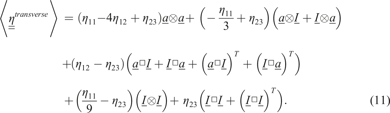
The method of orientation averaging was introduced by Advani and Tucker. ²⁴ In Equation (11) the dyadic product is described by the operator ⊗, defined as ${\left(A\otimes B\right)}_{ijkl}=A_{ij}{B}_{kl}$ , and the operator □ describes the box product: ${\left(A\square B\right)}_{ijkl}=A_{ik}{B}_{jl}$ .

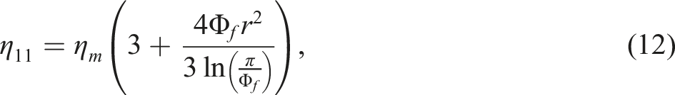
In this work the calculation of the three viscosities, axial elongational viscosity η₁₁, axial shear viscosity η₁₂, and transverse shear viscosity η₂₃, is conducted according to Pipes ²⁵ :

${\eta }_{11}={\eta }_m\left(3+\frac{4{\mathrm{\Phi }}_f{r}^2}{3\hspace{0.17em}\ln \left(\frac{\pi }{{\mathrm{\Phi }}_f}\right)}\right),$

(12)

${\eta }_{12}={\eta }_m\left(\frac{1+{\mathrm{\Phi }}_f}{1-{\mathrm{\Phi }}_f}\right),$

(13)

${\eta }_{23}={\eta }_m\left(\frac{1}{1-\sqrt{\frac{{\mathrm{\Phi }}_f}{{\mathrm{\Phi }}_{\max }}}}\right),$

(14)

with η _m representing the matrix viscosity, Φ _f representing the fiber volume fraction, Φ_max representing the maximum possible fiber fraction ( ${\mathrm{\Phi }}_{\max }=\pi /\left(2\sqrt{3}\right)$ for hexagonal packing), and r representing the aspect ratio of the fiber (r = L/D, where L is the fiber length and D is the fiber diameter). The indices of the viscosities η₁₁, η₁₂, and η₂₃ are defined as follows: 1 refers to in fiber direction, 2 refers to transverse in plane, and 3 refers to through thickness.

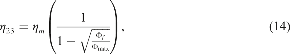
Wittemann ¹³ further defined:

${\eta }^{eff,iso}=\frac{1}{10}{\underset{\_}{\underset{\_}{\eta }}}^{eff}:{\underset{\_}{\underset{\_}{P}}}^2,$

(15)

with ${\underset{\_}{\underset{\_}{P}}}^2$ representing the second projection tensor of fourth order:

${\underset{\_}{\underset{\_}{P}}}^2=\underset{\_}{\underset{\_}{I}}-\underset{\_}{I}\otimes \underset{\_}{I}/3,$

(16)

and

${\underset{\_}{\underset{\_}{\eta }}}^{eff,iso}={\eta }^{eff,iso}\left[\begin{array}{llllll}4/3& -2/3& -2/3& 0& 0& 0\\ & 4/3& -2/3& 0& 0& 0\\ & & 4/3& 0& 0& 0\\ & & & 1& 0& 0\\ & & & & 1& 0\\ & symm.& & & & 1\end{array}\right].$

(17)

Finally, the viscous stress $\underset{\_}{\tau }$ is calculated, which was introduced in Equation (6) ¹³ :

$\begin{array}{l}\underset{\_}{\tau }={\underset{\_}{\underset{\_}{\eta }}}^{eff}:\underset{\_}{D}=\left({\underset{\_}{\underset{\_}{\eta }}}^{eff,iso}+{\underset{\_}{\underset{\_}{\eta }}}^{eff,aniso}\right):\underset{\_}{D}\\ =2{\eta }^{eff,iso}\left(\underset{\_}{D}-\frac{1}{3}tr{\left(\nabla \overrightarrow{u}\right)}^T\underset{\_}{I}\right)+{\underset{\_}{\underset{\_}{\eta }}}^{eff,aniso}:\underset{\_}{D}.\end{array}$

(18)

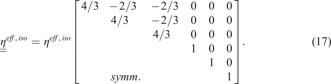
For UD tapes the fiber aspect ratio is typically very high, due to the continuous fibers. This leads to a very high axial elongational viscosity η₁₁ and high values on the tensor diagonal in the effective anisotropic viscosity ${\underset{\_}{\underset{\_}{\eta }}}^{eff,aniso}$ , since the fibers are highly oriented. This can lead to numerical instabilities when solving equation (5).

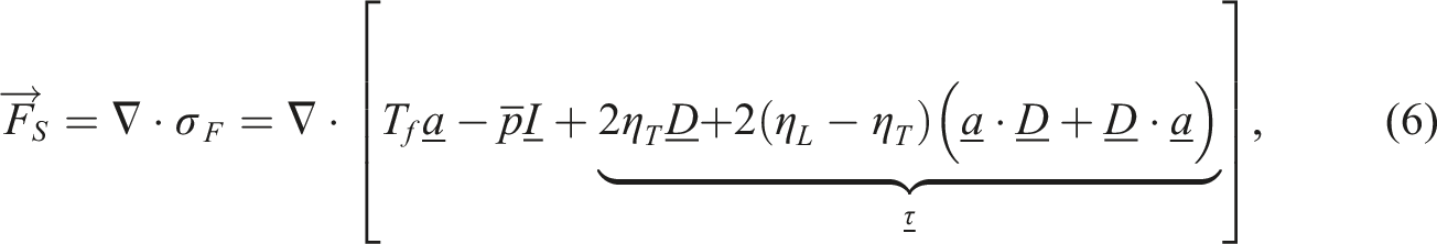
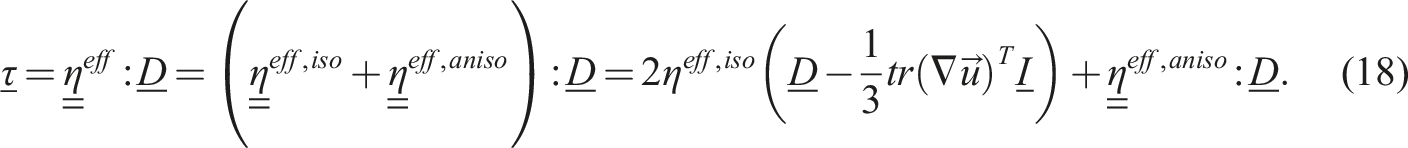
To avoid these instabilities an alternative solution was found: the viscous stress $\underset{\_}{\tau }$ is multiplied by the fiber direction tensor $\underset{\_}{a}$ component by component, which leads to an overall reduction of the viscous stress tensor $\underset{\_}{\tau }$ and is compensated by introducing the source term ${\overrightarrow{S}}_M$ in Equation (5).

In this work, the source term ${\overrightarrow{S}}_M$ describes the Darcy-Forchheimer-Law:

${\overrightarrow{S}}_M=\left({\eta }_m\overrightarrow{Da}+\frac{1}{2}\rho tr\left(\overrightarrow{u}·\overrightarrow{I}\right)\overrightarrow{F}\right)·\overrightarrow{u},$

(19)

where the first term in the parenthesis describes Darcy’s model, and the latter term describes Forchheimer’s model, which is only applicable for turbulent flows and therefore neglected here. In Equation (19) $\overrightarrow{Da}$ represents the Darcy coefficient which is defined as a flow resistance. If $\overrightarrow{Da}$ is set to a very high value, i.e. 1e10, in fiber direction it can be equated with the arbitrary fiber tension used in Roger’s model (see Equation (6)).

By replacing the effective isotropic viscosity ${\underset{\_}{\underset{\_}{\eta }}}^{iso}$ and the effective anisotropic viscosity ${\underset{\_}{\underset{\_}{\eta }}}^{aniso}$ by the transversal viscosity η _T and the longitudinal viscosity η _L , respectively, and the source term ${\overrightarrow{S}}_M$ of Equation (5) by the term representing an arbitrary fiber tension $\nabla ·\left(T_f\underset{\_}{a}\right)$ in Equation (6), Roger’s ²² approach is again fulfilled.

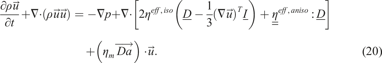
The final form of the thereby obtained momentum conservation equation (see Equation (5)) is given by:

$\begin{array}{l}\frac{\partial \rho \overrightarrow{u}}{\partial t}+\nabla ·\left(\rho \overrightarrow{u}\overrightarrow{u}\right)=\\ -\nabla p+\nabla ·\left[2{\eta }^{eff,iso}\left(\underset{\_}{D}-\frac{1}{3}{\left(\nabla \overrightarrow{u}\right)}^T\underset{\_}{I}\right)+{\underset{\_}{\underset{\_}{\eta }}}^{eff,aniso}:\underset{\_}{D}\right]+\left({\eta }_m\overrightarrow{Da}\right)·\overrightarrow{u}.\end{array}$

(20)

The computational mesh is designed in such a way that each cell in the thickness direction contains a single tape layer. Furthermore, it is assumed that the fibers are rigid and do not change their orientation. The corresponding models for fiber reorientation are therefore ignored.

The conservation of the inner energy e is considered by:

$\frac{\partial \rho e}{\partial t}+\nabla ·\rho \overrightarrow{u}e-\left[\nabla ·\overrightarrow{u}p\right]+\frac{\partial \rho K}{\partial t}+\nabla ·\rho \overrightarrow{u}K=\nabla ·{\alpha }_{th,eff}\nabla e+\rho S,$

(21)

where the first three terms describe the change in inner energy e with time, convection of the inner energy e and compression heating. The remaining terms on the left-hand side represent the change in mechanical energy K with time and the convection in the mechanical energy K, respectively. On the right-hand side the heat conduction is included, with α_th,eff being the effective thermal diffusivity. Crystallization or melting energy can be included with the optional source term S. However, this effect was omitted in this work, since an amorphous matrix material was considered.

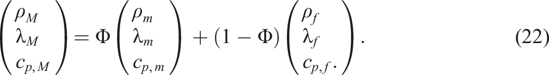
The material properties of the mixture of matrix and fibers, that is, density ρ _M , thermal conductivity λ _M , and specific heat capacity c_(p,M), are calculated using the rule of mixture (Equation (22)). ²⁶

$\left(\begin{array}{l}{\rho }_M\\ {\mathrm{\lambda }}_M\\ c_{p,M}\end{array}\right)=\mathrm{\Phi }\left(\begin{array}{l}{\rho }_m\\ {\mathrm{\lambda }}_m\\ c_{p,m}\end{array}\right)+\left(1-\mathrm{\Phi }\right)\left(\begin{array}{l}{\rho }_f\\ {\mathrm{\lambda }}_f\\ c_{p,f}.\end{array}\right).$

(22)

Acquisition of material data as well as the corresponding boundary conditions that contribute to the thermodynamic behavior were described in more detail in. ⁶

Initial and boundary conditions

In the consolidation process, a force or pressure is usually applied to act on the composite part during heating and cooling. To model the flow behavior resulting from the pressure p(t) acting on the specimen, a boundary condition was implemented to calculate p(t), over a projected area A _sample (t), resulting from the magnitude of the force applied $\left|\overrightarrow{F}\right|\left(t\right)$ :

$p\left(t\right)=\frac{\left|\overrightarrow{F}\right|\left(t\right)}{A_{sample}\left(t\right)}.$

(23)

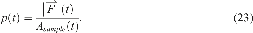
Since the sample is squeezed during processing, its projected area A _sample (t) changes with time, and the calculated pressure p(t) changes accordingly. In reality, the set pressure/force does not remain constant throughout a trial, but varies due to the movement of the piston of the heating/cooling plates. Therefore, the boundary condition reads the force from a table with corresponding time values that was recorded during the experiments.

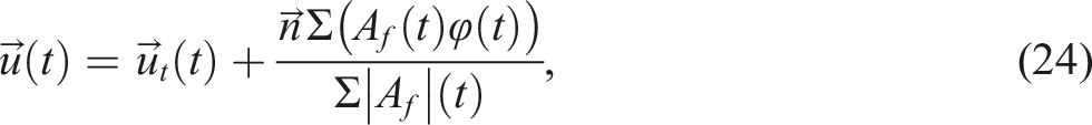
A slip boundary condition is set at the interfaces between the specimen and the tool, since a release agent was used in the experiments to prevent the specimen from sticking to the tool. At the interface where the pressure acts on the specimen, the boundary condition calculates the mean velocity according to the pressure, using the flux φ(t):

$\overrightarrow{u}\left(t\right)={\overrightarrow{u}}_t\left(t\right)+\frac{\overrightarrow{n}\mathrm{\Sigma }\left(A_f\left(t\right)\phi \left(t\right)\right)}{\mathrm{\Sigma }\left|A_f\right|\left(t\right)},$

(24)

where ${\overrightarrow{u}}_t\left(t\right)$ is the tangential component of the velocity, which captures the friction-free slip condition, $\overrightarrow{n}$ is the normal vector of the interface, A _f (t) is the area of each cell face at the boundary, and |A _f |(t) is the the magnitude of the face areas.

The compression of the specimen, resulting from the pressure, is modeled by a cell displacement $\left(\overrightarrow{d}\left(t\right)\right)$ boundary condition, which calculates the integral of the interface velocity ${\overrightarrow{u}}_i\left(t\right)$ over time:

$\overrightarrow{d}\left(t\right)={\int }_{t-1}^t{\overrightarrow{u}}_i\left(t\right) dt.$

(25)

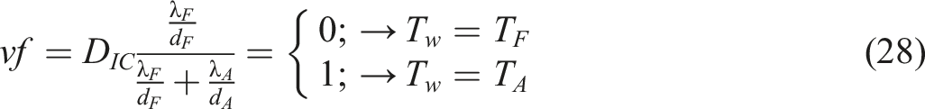
To model the heat transfer between heating/cooling plates, tools and composite, a boundary condition for the heat conduction is used. To this end, a value fraction vf is calculated at the interface of two regions (solid/solid or solid/fluid) and used to determine the wall temperature T _w :

$vf=D_{IC}\frac{\frac{{\mathrm{\lambda }}_F}{d_F}}{\frac{{\mathrm{\lambda }}_F}{d_F}+\frac{{\mathrm{\lambda }}_S}{d_S}}=\{\begin{array}{l}0;\to T_w=T_F.\\ 1;\to T_w=T_S.\end{array}$

(26)

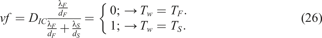
The indices F and S refer to the fluid and solid regions, respectively, and d describes the thickness of a finite volume element at the corresponding boundary wall. An impeded heat transfer due to surface roughness is considered by the degree of intimate contact D _IC in equation (26):

$D_{IC}=\frac{1}{1+\frac{w_0}{b_0}}{\left[1+5\left(1+\frac{w_0}{b_0}\right){\left(\frac{a_0}{b_0}\right)}^2{\int }_0^{tc}\frac{P_{app}\left(t\right)}{{\eta }_0\left(T\left(t\right)\right)}dt\right]}^{\frac{1}{5}}.$

(27)

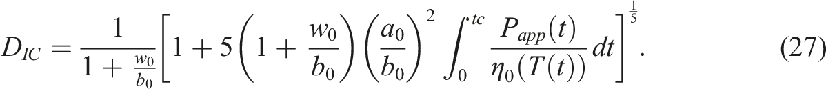
The degree of intimate contact is based on the assumption that perfect contact is not immediately achieved due to surface roughness. ²⁷ It is used for a simplified view of the surface roughness, which is assumed to be approximately rectangular and described by the initial geometric values: the distance between two rectangles w₀, the width b₀ and the height a₀ of a rectangle, the applied pressure P _app and the temperature-dependent dynamic zero viscosity η₀(T).^28,9,29

Assuming that there is no ideal contact between the heating/cooling plates and the tools that limits heat conduction, a thin layer of air is considered in the boundary condition, which yields:

$vf=D_{IC}\frac{\frac{{\mathrm{\lambda }}_F}{d_F}}{\frac{{\mathrm{\lambda }}_F}{d_F}+\frac{{\mathrm{\lambda }}_A}{d_A}}=\{\begin{array}{l}0;\to T_w=T_F\\ 1;\to T_w=T_A\end{array}$

(28)

where the index A refers to the air layer.

Solution procedure

Figure 4 shows the order in which the equations described above are solved.

Figure 4.

Solution procedure for simulating the consolidation process.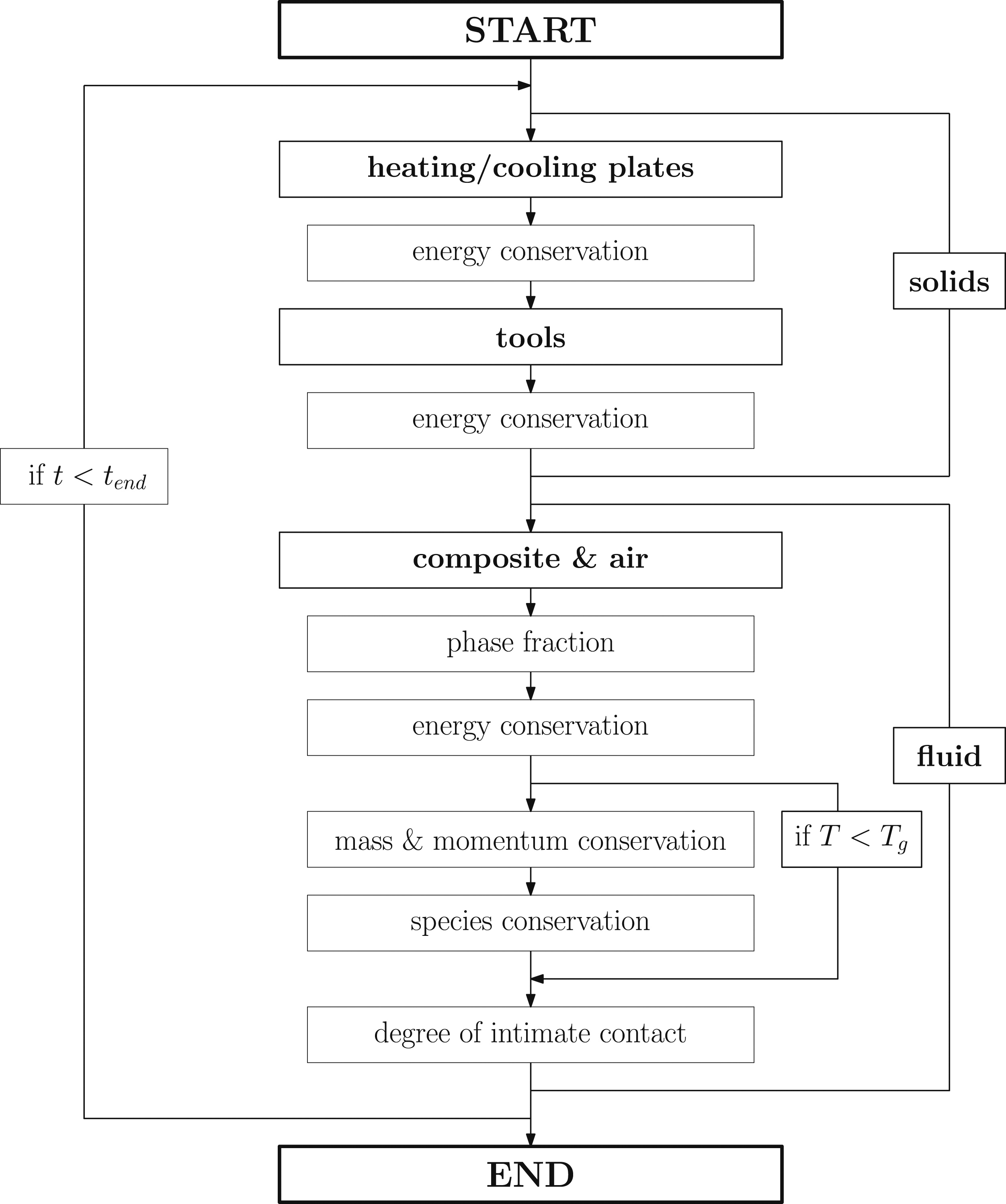

First, the energy conservation (Equation (1)) is solved for the solids (heating/cooling plates and tools). Equations (3)–(5), and (21) are then solved for the fluid phases (air and composite). The anisotropic squeeze flow is calculated within the mass and momentum conservation as described above. Since the focus of this work was on the anisotropic squeeze flow, the description of the species conservation (Figure 4) was omitted.

In order to avoid numerical instabilities and also for simplification, a threshold is set with respect to the composite temperature. If the temperature of the composite is lower than a user-defined temperature, i.e. T _g , the calculations for mass and momentum conservation are skipped.

The OpenFOAM^® version used in this work was not able to handle fourth-order tensors. Due to the assumption of transverse isotropy, the anisotropic viscosity tensor ${\underset{\_}{\underset{\_}{\eta }}}^{eff,aniso}$ shows right-hand, left-hand and main symmetry. It can therefore be expressed in Voigt notation and split into three second-order tensors, as shown in Figure 5.

Figure 5.

Anisotropic viscosity tensor 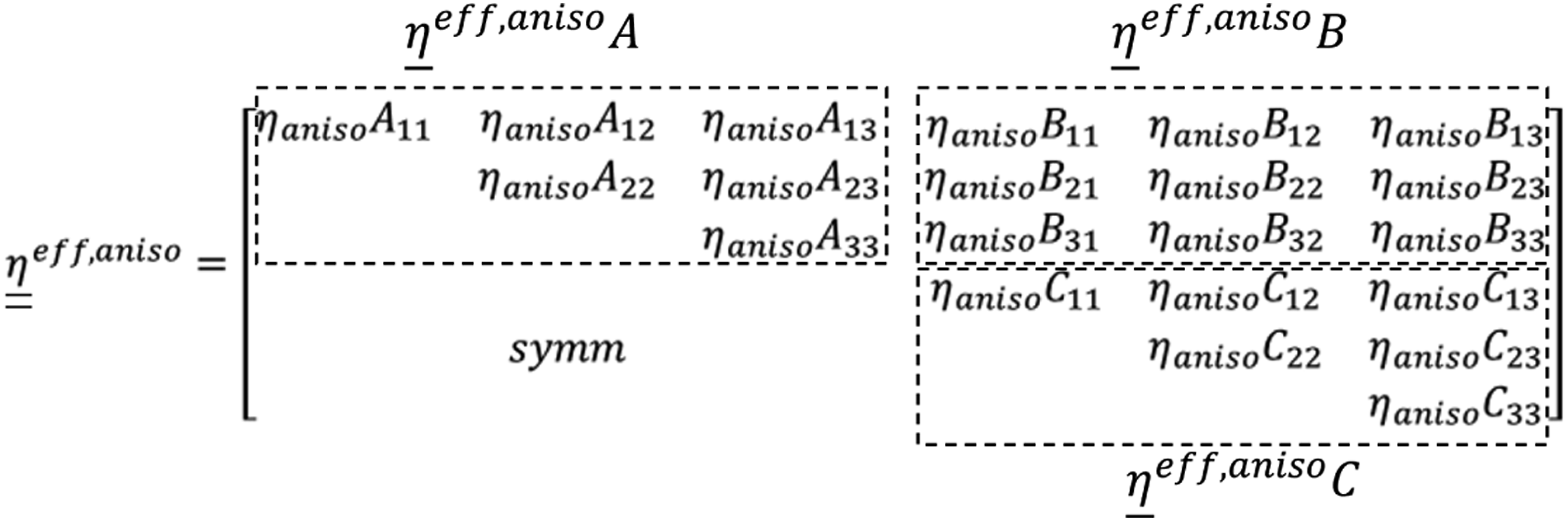${\underset{\_}{\underset{\_}{\eta }}}^{eff,aniso}$ expressed in Voigt notation and split into three second-order tensors ${\underset{\_}{\eta }}^{eff,aniso}A$ , ${\underset{\_}{\eta }}^{eff,aniso}B$ , and ${\underset{\_}{\eta }}^{eff,aniso}C$ .

Experimental

Specimen

The specimens used consisted of several layers of polycarbonate UD tapes with 44% carbon fiber by volume and a nominal thickness of 0.175 mm. To determine the influence of the fiber direction on squeezing, various layups were test, as summarized in Table 1.

Table 1.

Description of the specimens and layups used.

Name	Layers	Layup
UD	12	[0°|0°|0°|0°|0°|0°]S
Crossply90	12	[0°|90°|0°|90°|0°|90°]S
Crossply45	12	[-45°|+45°|-45°|+45°|-45°|+45°]S
Quasiisotropic	8	[0°|-45°|+45°|90°]S

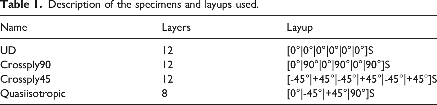
The experiments labeled “UD” and “Crossply90” were performed with 40 × 40 mm² and 30 × 30 mm² specimens. Due to the high level of effort involved in producing specimens with ±45° layers, the experiments labeled “Crossply45” and “Quasiisotropic” were performed with 30 × 30 mm² specimens only.

Experimental setup

The experiments to validate the anisotropic squeeze flow were conducted using a laboratory-scale consolidation unit with two pneumatic presses, one for heating and one for cooling (see Figure 6).

Figure 6.

Lab-scale consolidation unit, consisting of heating unit, cooling unit and data-recording unit.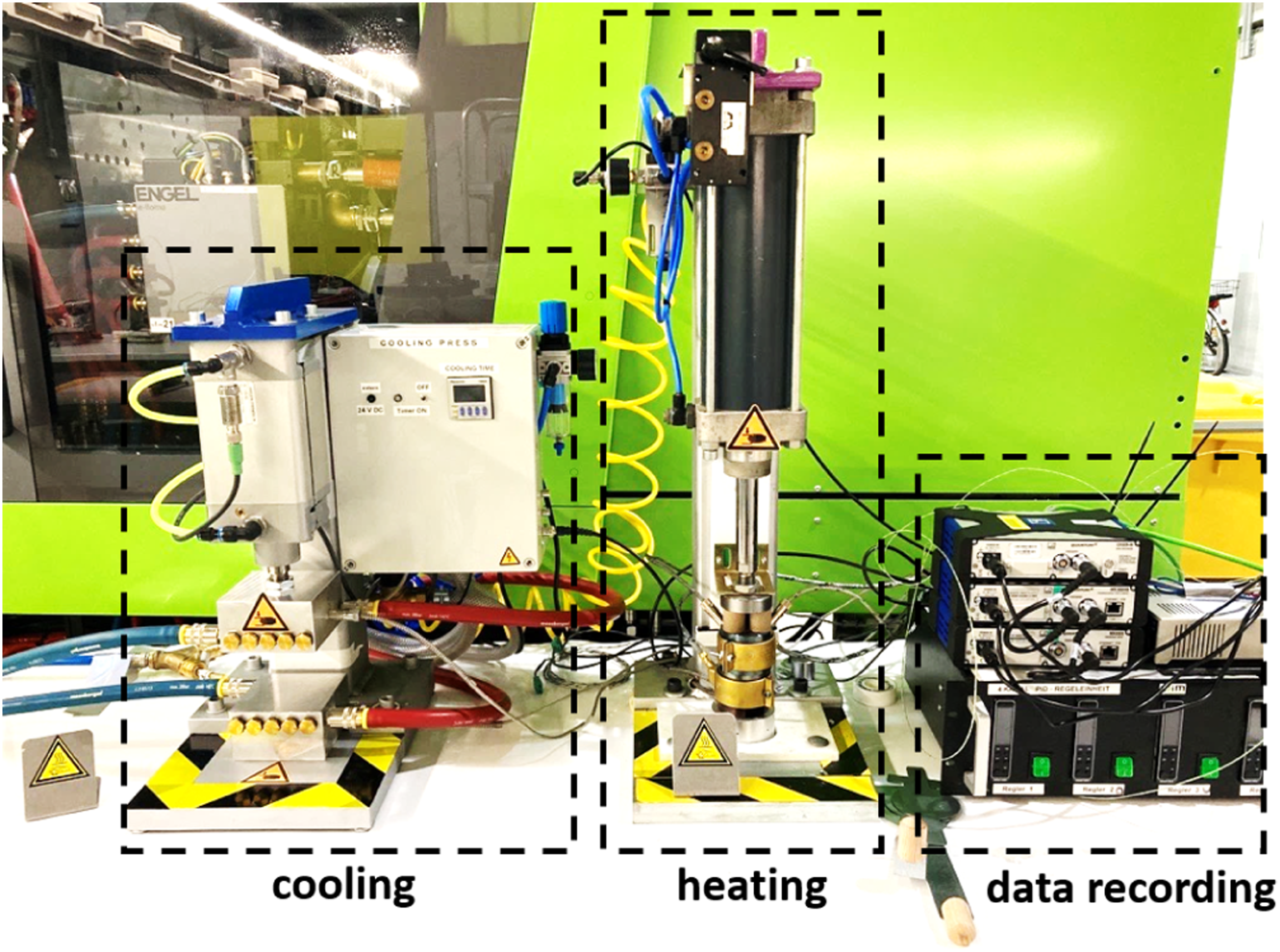

The heating press was equipped with heating sleeves at the upper and lower stamps. Cooling channels were incorporated into the stamps of the cooling press. A temperature control unit of an injection molding machine was used for cooling. A specimen was placed between two aluminum plates and transported manually from the heating unit to the cooling unit.

The data from (i) temperature sensors (thermocouple type J) incorporated into each heating and cooling stamp and (ii) pressure sensors (PT5403, IFM, Essen, Germany) placed at the pneumatic aggregate at the heating and cooling presses was recorded by means of an HBM data-recording system (QuantumX CS22B-W, HBM, Darmstadt, Germany).

To record the squeezing of the specimen during consolidation, a camera was placed in front of each press. The video quality was set to 4K, leading to a resolution of 26 pixels/mm and 30 fps (frames per second). Gray-scale analysis using a custom Python script was then performed to determine the shape of the specimen for each frame. The output was a list giving (i) specimen length and (ii) specimen thickness over time.

Since volume constancy is assumed due to incompressibility, the geometric change of the specimen in the direction perpendicular to the image plane is neglected.

Figure 7 shows the setup.

Figure 7.

Frame of a video recorded during an experiment, showing the specimen, upper and lower stamps, the heating sleeves, and the transfer plates.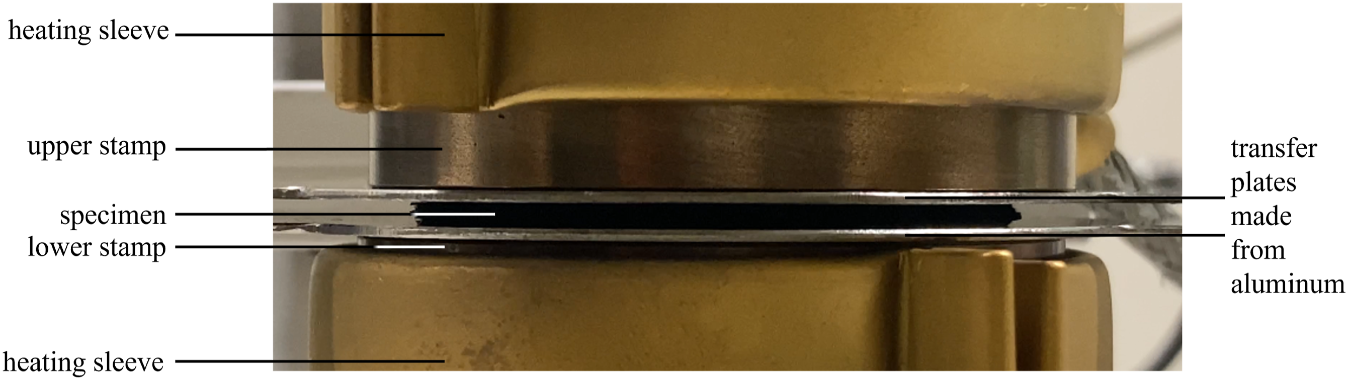

Figure 8 illustrates the domain of interest as determined by the Python script and then used for comparison with the simulation.

Figure 8.

Domain of interest with length and thickness, quantified by the Python script.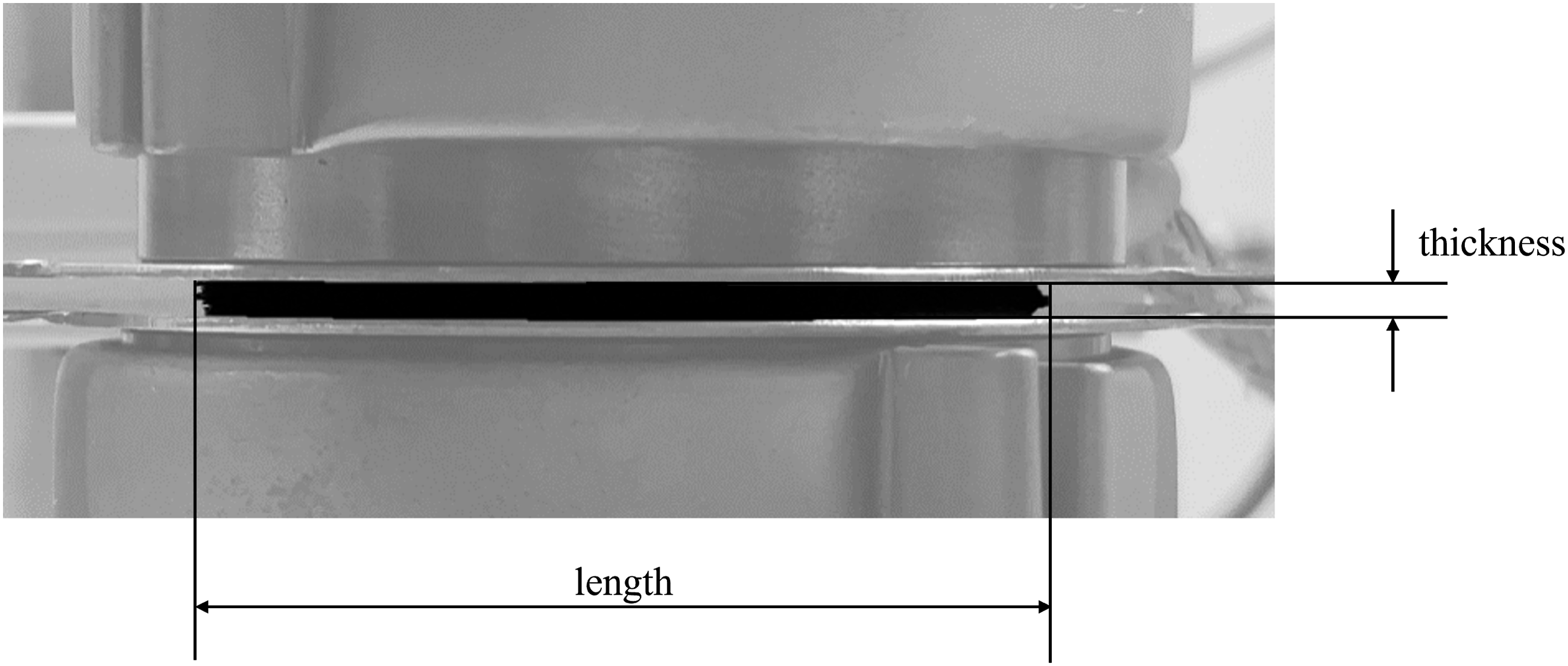

Parameter settings

Since this work focused exclusively on the influence of fiber orientation on the squeeze flow, all experiments were performed at one process setting: a heating-press temperature T_H of 250°C, a cooling-press temperature T_C of 60°C and a heating- and cooling-press pressure of 20 bar for the 40 × 40 mm² specimens and 35 bar for the 30 × 30 mm² specimens (see Table 2). The different pressures are due to the different specimen sizes, as the set pressure acting on the pneumatic piston was kept constant.

Table 2.

Used process settings, which are heating temperature T_H, cooling temperature T_C, heating pressure p_H, and cooling pressure p_C.

TH (°C)	TC (°C)	pH (bar)	pC (bar)
250	60	20 for 40 × 40 mm2,	20 for 40 × 40 mm2,
		35 for 30 x 30 mm2	35 for 30 x 30 mm2

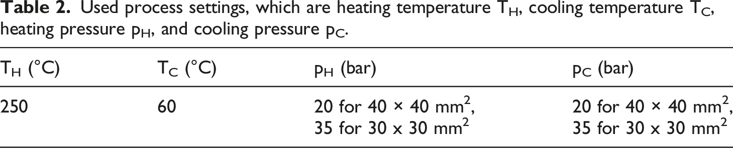
Three specimens were used for each run.

Results

Experiments

To ensure that the matrix was in a processable state (i.e., that the temperature at the core of the specimen was higher than the glass-transition temperature of 147°C) measurements were taken with a thermocouple (type K) at the core of the specimen. Figure 9 shows the temperatures recorded for a process with 250°C heating temperature, 60°C cooling temperature, 10 bar pressure at the heating press and 30 bar pressure at the cooling press. It can be seen that 2.3 s after the cooling process started, the temperature dropped below the glass-transition temperature, which means that the specimen was in a solid state and material flow in the form of squeeze flow was no longer possible.

Figure 9.

(a) Overview of an experiment with 250°C heating temperature, 60°C cooling temperature, 10 bar pressure at the heating press, and 30 bar pressure at the cooling press, and (b) detail of the beginning of the cooling step, with a horizontal dashed line indicating a temperature (T = 140°C) below the glass-transition temperature (T _g = 147°C) and two vertical dashed lines indicating, respectively, the start of the cooling process and the time point at which the layup temperature dropped below the glass transition temperature.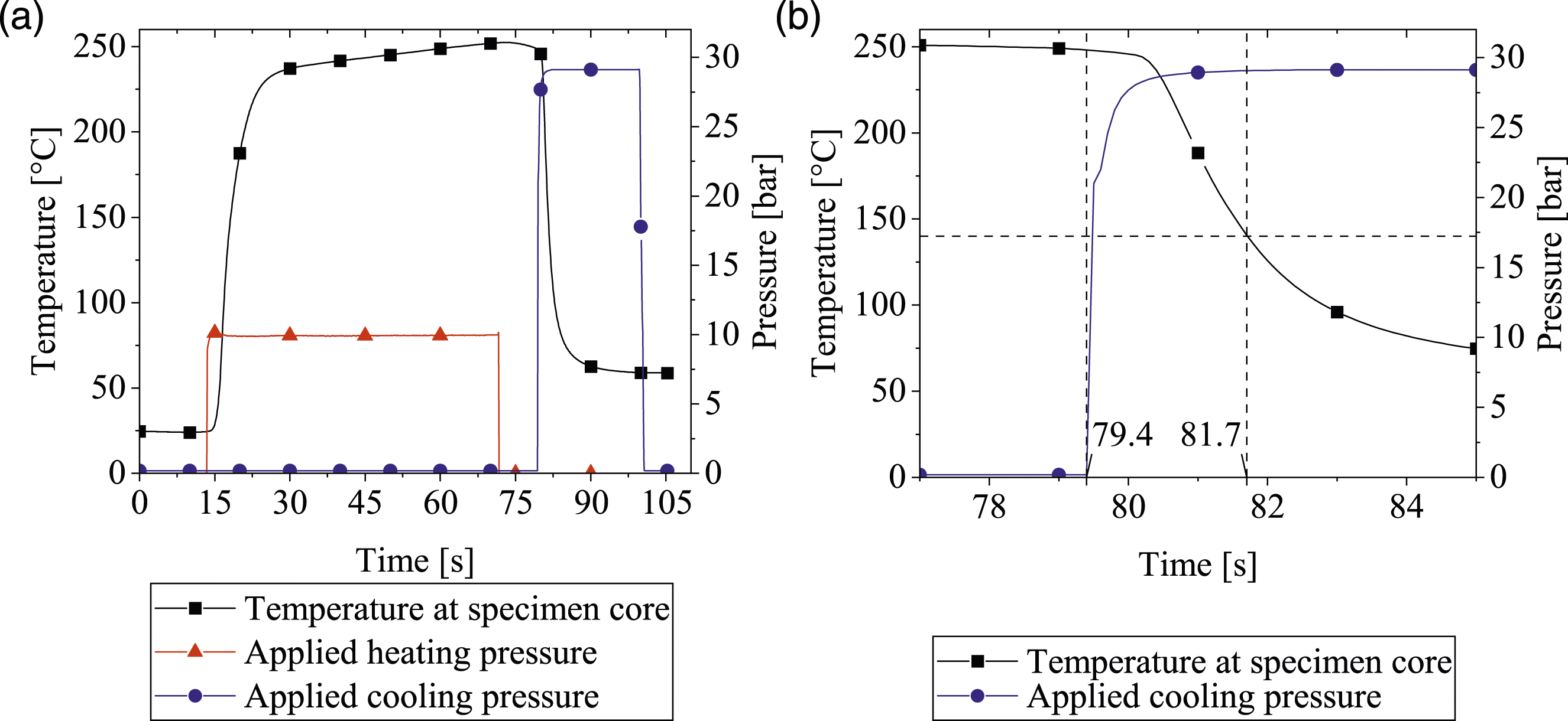

Figure 10(a) and (b) show that, due to the rapid temperature drop described above, no significant change in specimen thickness or length was detected by the camera during the cooling cycle. This work therefore focused on the heating phase of the consolidation process. Notably, there is a slight increase in thickness between 65 s and 72 s, which is caused by measurement inaccuracy.

Figure 10.

(a) Thickness and length of the specimen during a process with 250°C heating temperature, 60°C cooling temperature, 10 bar pressure at the heating press and 30 bar pressure at the cooling press, and (b) detail of the transition from heating to cooling. The dashed lines indicate the period for which the core temperature of the specimen was higher than the glass-transition temperature (T _g = 147°C).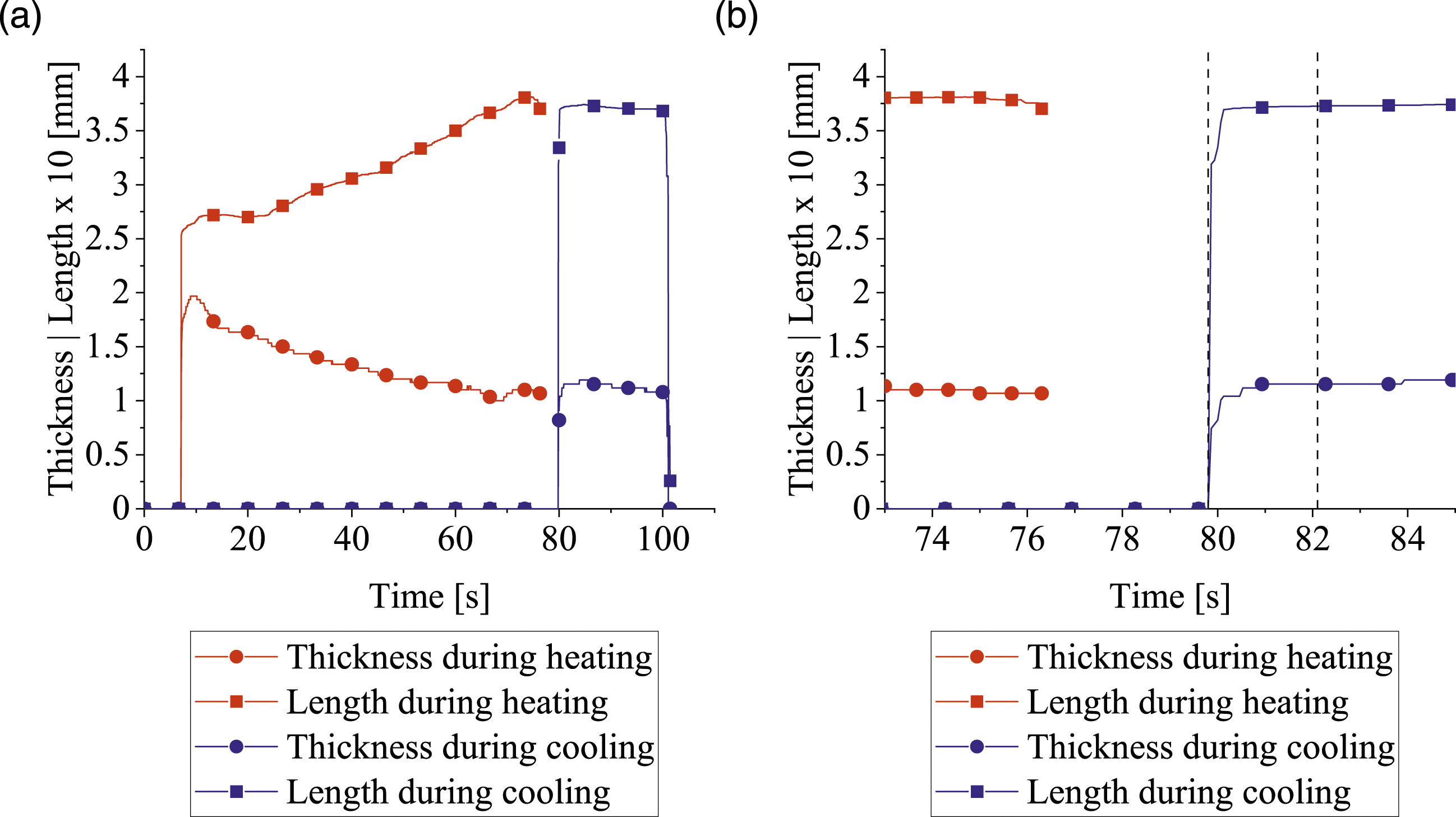

Figure 11 shows the result of a test with a 30 × 30 mm² UD layup specimen in the heating press: The pressure was not constant throughout the experiment, but was excessive at the beginning and leveled off toward the end of the test. As the deviation from the set pressure was less than 5%, this was not investigated further. For all specimens, there was an initial drop in thickness at the beginning, which was identified as a compaction of the solid material, because the layups were slightly warped. Since the temperature at the core of the specimen reached the glass-transition temperature roughly 8 seconds after pressure had been applied (see Figure 10), it can be excluded that this initial change in length was due to squeeze flow. The drop in thickness, length, and pressure at the end of each measurement indicates removal of the specimen from the heating press and thus pressure release.

Figure 11.

Result of a test performed with a 30 × 30 mm² UD layup, showing the mean values of thickness and length of the specimen during the test in the heating press and the pressure applied.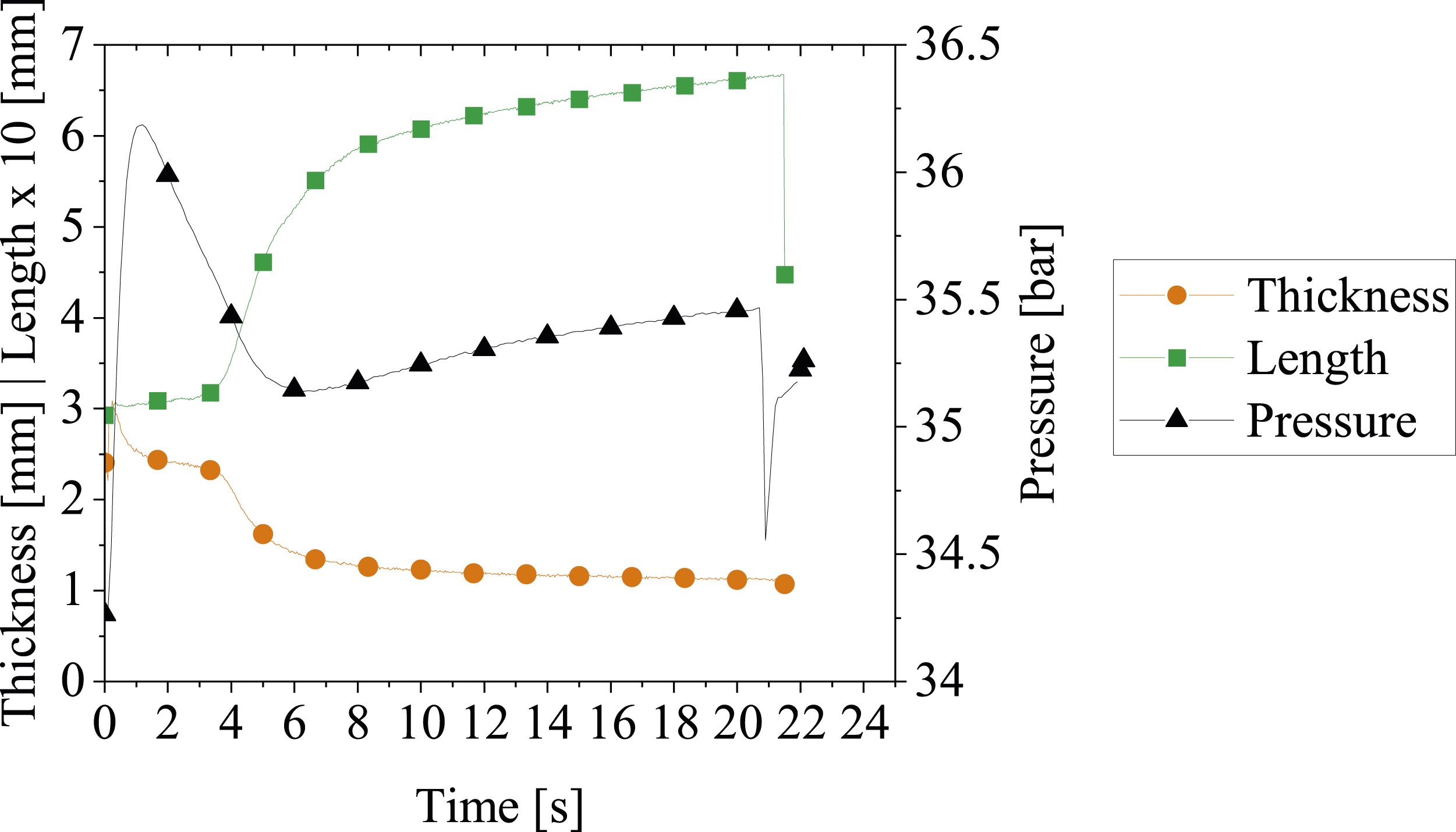

The results for all specimens are shown in Figure 10. It can clearly be seen that the changes in length and thickness of the crossply and quasi-isotropic layups (Figure 12(a), (b), (e) and (f)) were linear, while the changes in length and thickness of the “UD” layups (Figure 12 (c) and (d)) can be better described by a logarithmic function. Initially, the length increased dramatically while the thickness decreased accordingly, reaching a plateau after about 7.5 seconds. Note the very low standard deviation of the length change of the “Quasiisotropic” layup (Figure 12(f)).

Figure 12.

Results of all tests, showing the mean values and deviations of the changes in thickness and length of the specimens during the test in the heating press for “Crossply90” with areas of 40 × 40 mm² (a) and 30 × 30 mm² (b), “UD” layups with areas of 40 × 40 mm² (c) and 30 × 30 mm² (d), “Crossply45” with an area of 30 × 30 mm² (e), and “Quasiisotropic” with an area of 30 × 30 mm² (f).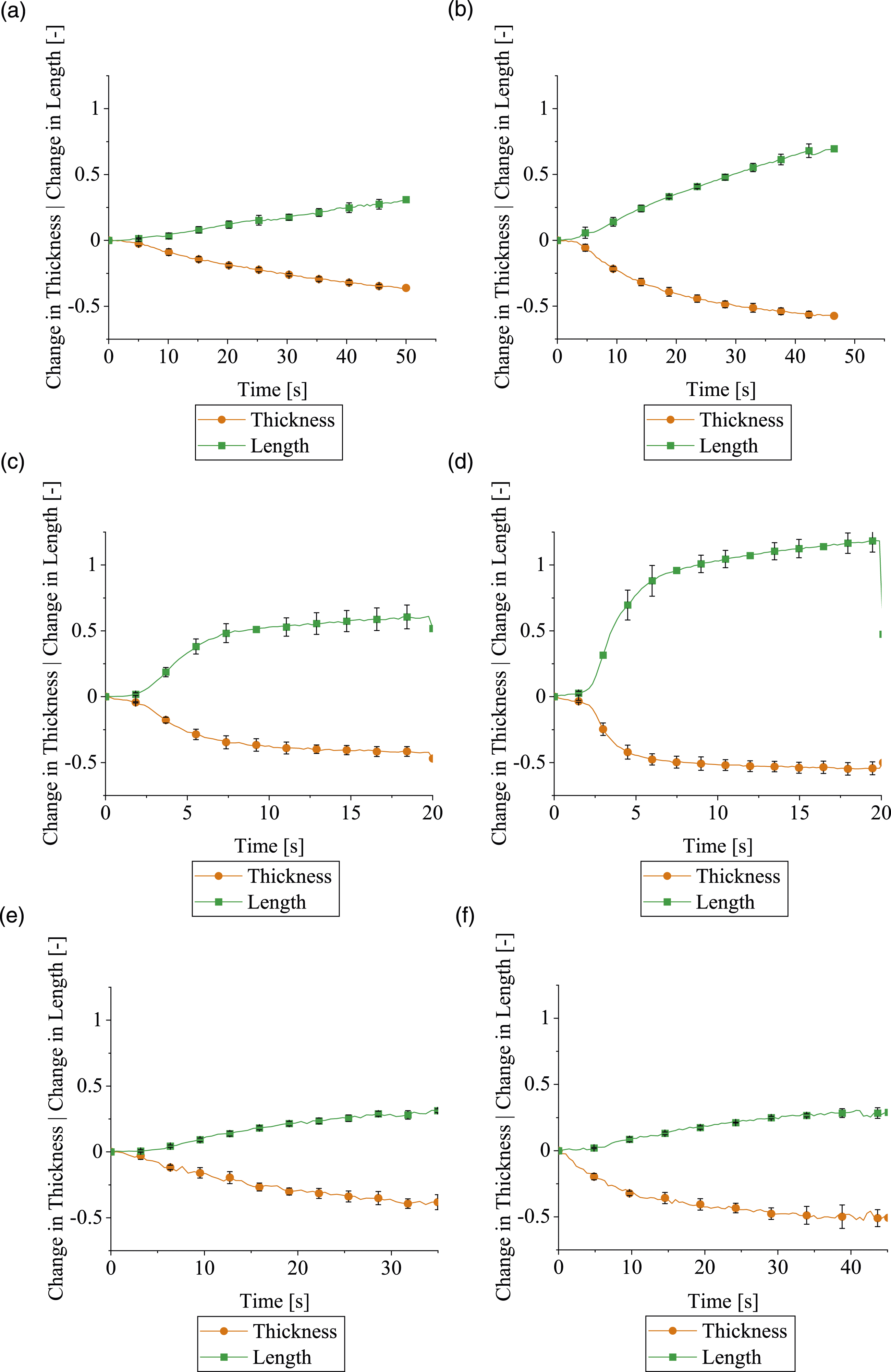

Simulation

To ensure that the thermodynamic behavior was correctly modeled, we compared our results with the thermocouple data recorded at the core of a specimen. Figure 13 shows the comparison for a temperature of 250°C set at the heating press: The simulation deviates from the experimental data by a maximum of 12% at around 5 seconds, while the difference in time at which the glass-transition temperature was exceeded (T = 147°C) is 0.34 seconds.

Figure 13.

Comparison of specimen core temperatures (between layers 6 and 7) in simulation and experiment. The dashed line indicates the glass-transition temperature at 147°C.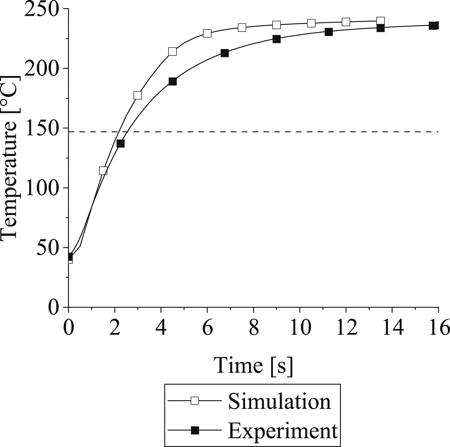

Figure 14 shows that for the 40 × 40 mm² and 30 × 30 mm² “Crossply90” specimens, the simulation reproduced the linear behaviors of the changes in length and thickness.

Figure 14.

Comparison of the changes in thickness and length of the 40 × 40 mm² (a) and 30 × 30 mm² (b) “Crossply90” specimens during heating in simulation and experiment.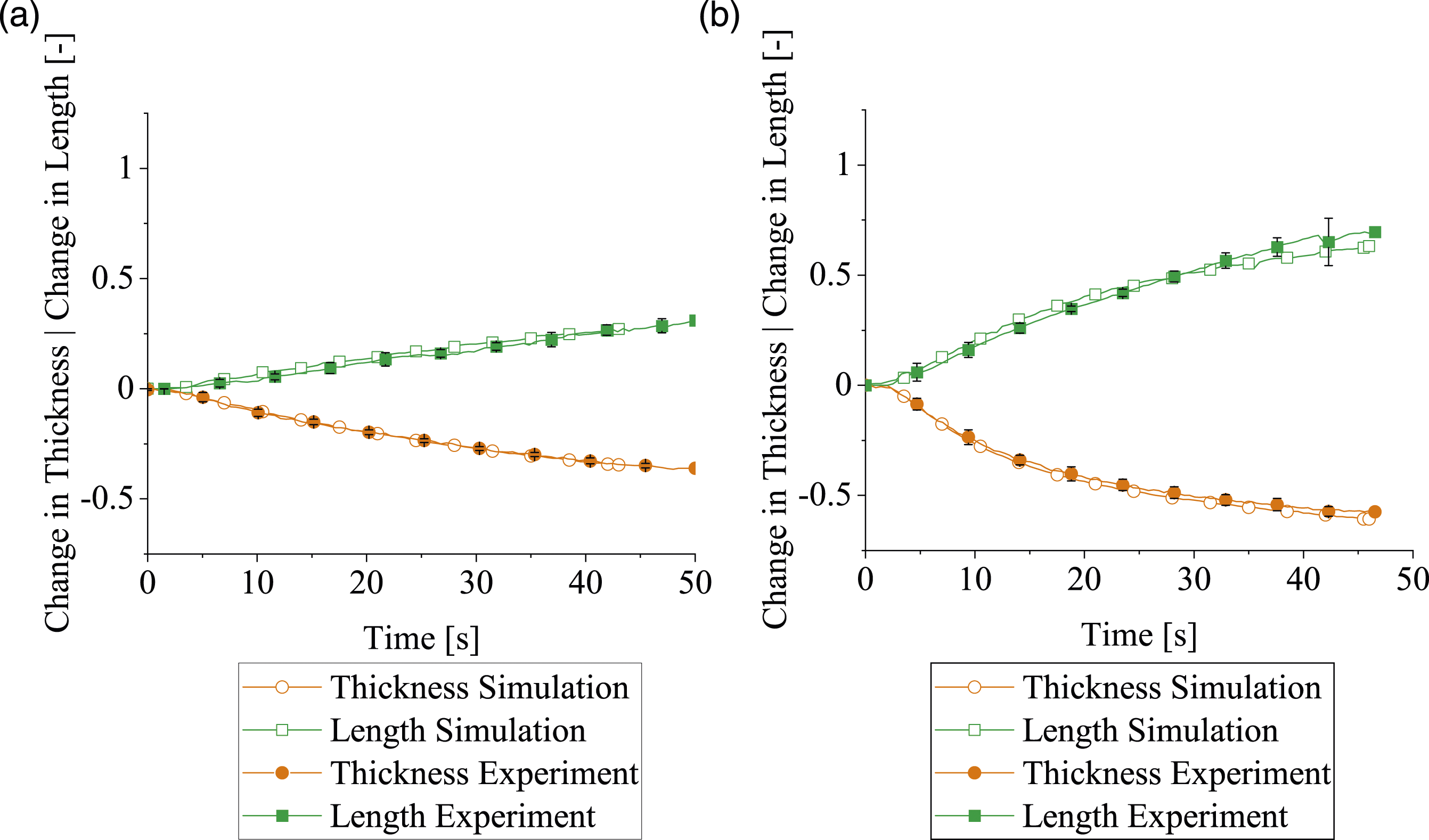

Due to numerical instabilities, the simulation for the 40 × 40 mm² “Crossply90” specimen was terminated before the set end time.

Figure 15 illustrates that for change in thickness of the “UD” specimens, the simulation is in good agreement with the experiment. For the change in length, however, the simulation deviates from the experiment, as the experimental results began to plateau, while the simulation results continued to increase. Again, due to numerical instabilities, the simulation was terminated before the set end time in both cases. These numerical instabilities occur because the case where all fibers are oriented in one direction is a mathematical extreme for the anisotropic viscosity model.

Figure 15.

Comparison of the changes in thickness and length of the 40 × 40 mm² (a) and 30 × 30 mm² (b) “UD” specimens during heating in simulation and experiment.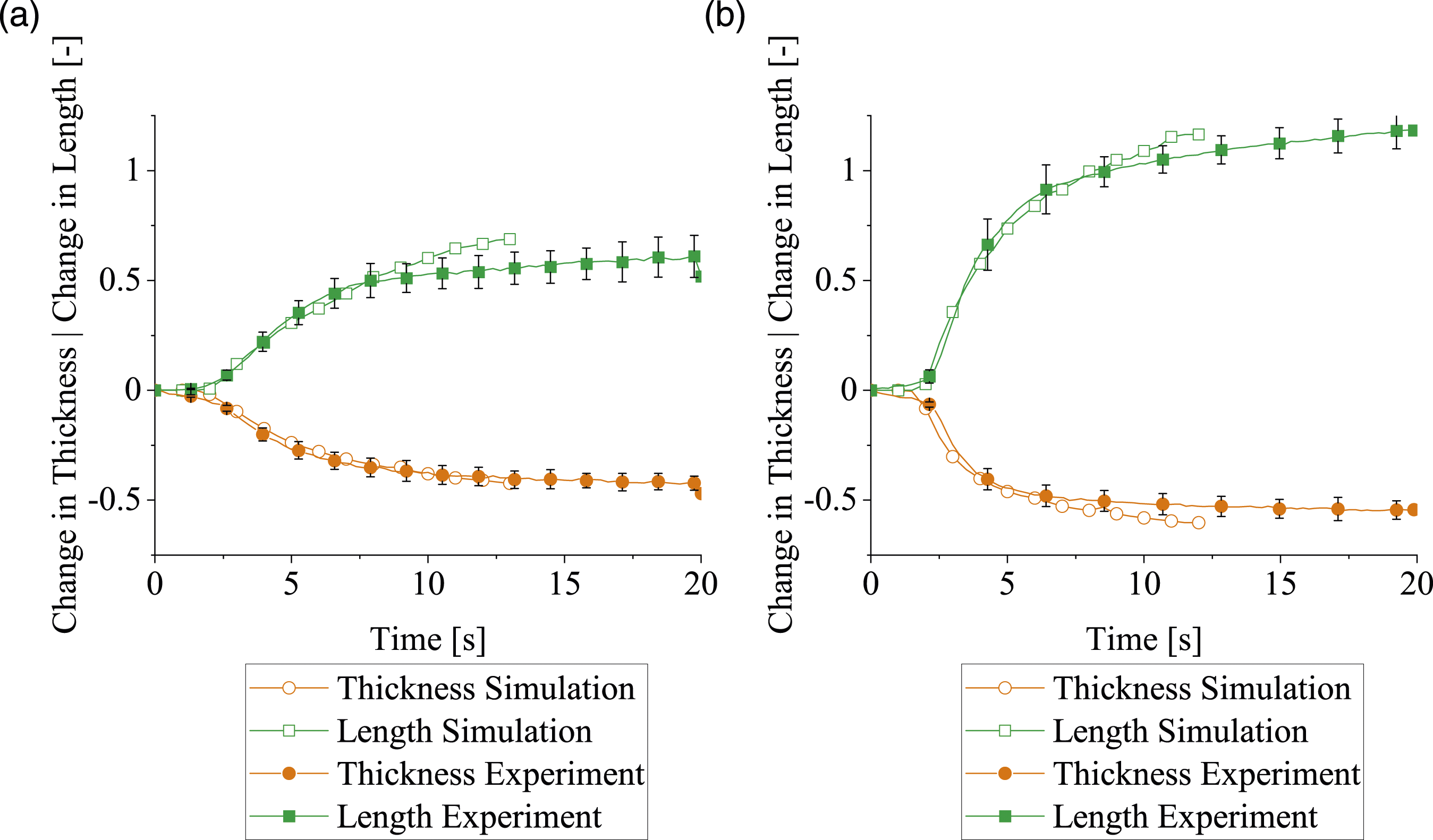

Figure 16 shows that for both cases, 30 × 30 mm² “Crossply45” and “Quasiisotropic”, the simulation data is in good accordance with the experimental data. While for “Quasiisotropic” the changes in thickness and length towards the end were overestimated by the simulation, for “Crossply45” only the change in thickness was overestimated by the simulation.

Figure 16.

Comparison of the changes in thickness and length for “Crossply45” (a) and “Quasiisotropic” (b) specimens during heating.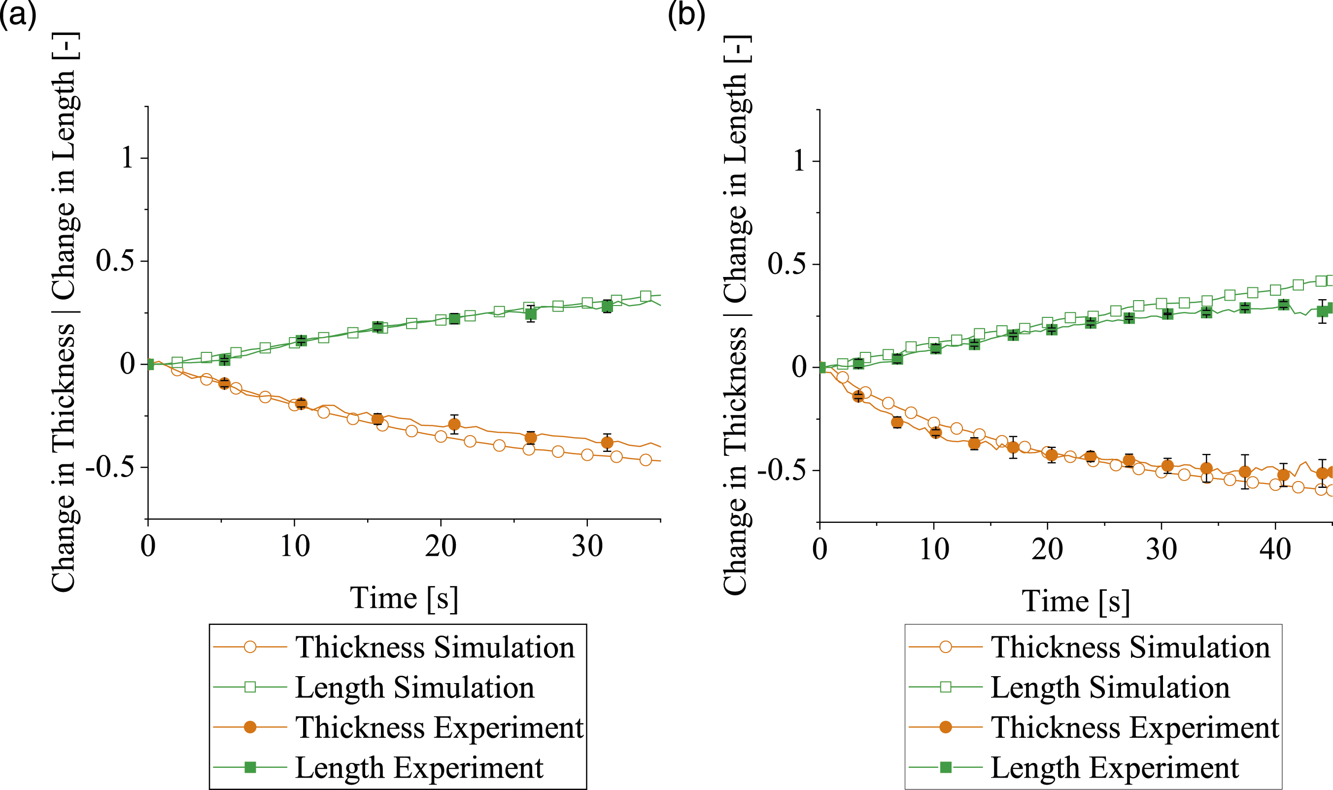

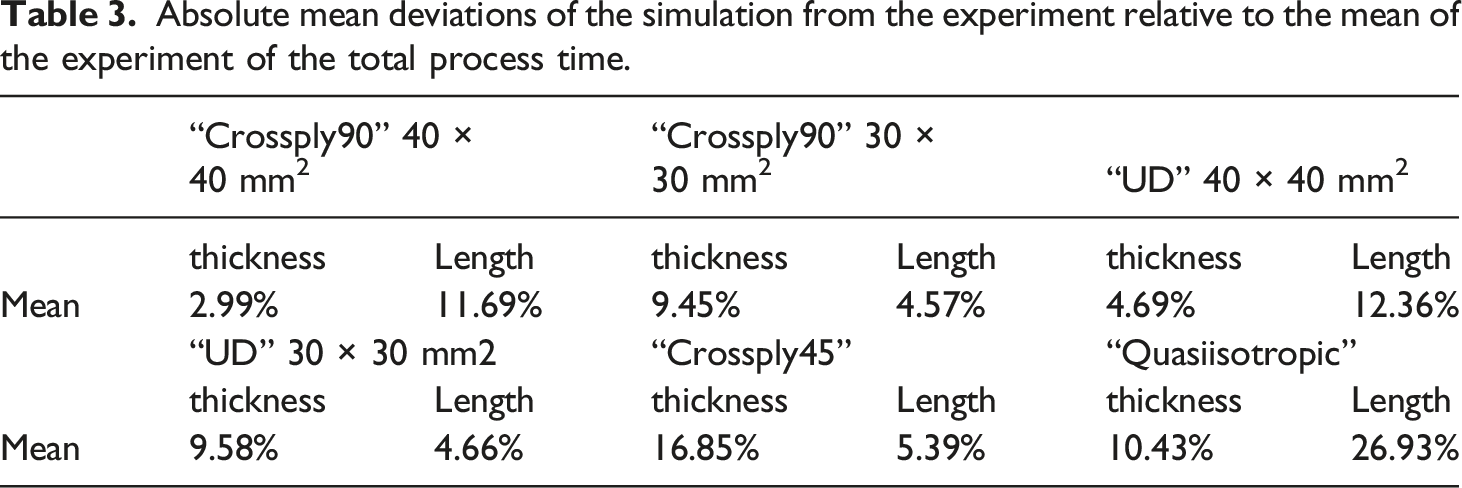
The mean divergences between simulation and experiment relative to the mean of the experiment of the total process time are listed in Table 3. The smallest deviation over the entire process time for the change in specimen thickness was 2.99% for the 40 × 40 mm² “Crossply90”, while the smallest deviation for the change in length was 4.66% for the 30 × 30 mm² “Crossply90”. The greatest deviations over the whole process time were found for “Crossply45” for the change in thickness (16.85%) and for “Quasiisotropic” for the change in length (26.93%).

Table 3.

Absolute mean deviations of the simulation from the experiment relative to the mean of the experiment of the total process time.

	“Crossply90” 40 × 40 mm2		“Crossply90” 30 × 30 mm2		“UD” 40 × 40 mm2
	thickness	Length	thickness	Length	thickness	Length
Mean	2.99%	11.69%	9.45%	4.57%	4.69%	12.36%
	“UD” 30 × 30 mm2		“Crossply45”		“Quasiisotropic”
	thickness	Length	thickness	Length	thickness	Length
Mean	9.58%	4.66%	16.85%	5.39%	10.43%	26.93%

In practical applications, the difference at the final time point is of interest, i.e. when the experiment or simulation is finished. Since in some cases the simulation was terminated too early due to numerical instabilities, the last data point of the simulation was used for comparison in this work.

As shown in Table 4, the smallest deviations were found for the 40 × 40 mm² “Crossply90” specimen, while the greatest deviations were observed for “Crossply45” in terms of thickness change and for “Quasiisotropic” in terms of length change.

Table 4.

Absolute mean deviations of the simulation from the experiment with respect to the mean of the experiment for the last common data point.

	“Crossply90” 40 × 40 mm2		“Crossply90” 30 × 30 mm2		“UD” 40 × 40 mm2
	thickness	Length	thickness	Length	thickness	Length
Mean	0.74%	0.84%	14.19%	8.66%	6.08%	23.77%
	“UD” 30 × 30 mm2		“Crossply45”		“Quasiisotropic”
	thickness	Length	thickness	Length	thickness	Length
Mean	10.77%	1.66%	16.74%	3.00%	16.53%	48.19%

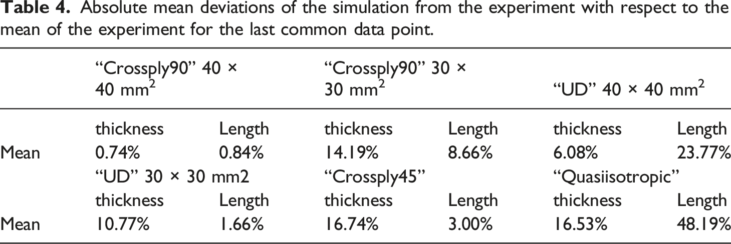
Figure 17 shows a qualitative comparison of the specimens after consolidation and at the end of the simulation. The comparison for the 40 × 40 mm² “Crossply90” case (a) shows good agreement, but for the 30 × 30 mm² “Crossply90” case (b) sliding of the individual layers and the formation of a cross shape were not adequately modeled. The simulation results of (c) and (d) resemble the experimental results. While the results were also in good agreement for the “Quasiisotropic” layup, the formation of the corners in the “Crossply45” case was underestimated by the simulation.

Figure 17.

Comparison between experiment (left) and simulation (right) in terms of final specimen shape for “Crossply90” with areas of 40 × 40 mm² (a) and 30 × 30 mm² (b), “UD” layups with areas of 40 × 40 mm² (c) and 30 × 30 mm² (d), the 30 × 30 mm² “Crossply45” layup (e), and the 30 × 30 mm² “Quasiisotropic” layup (f). The dashed squares indicate the original specimen size.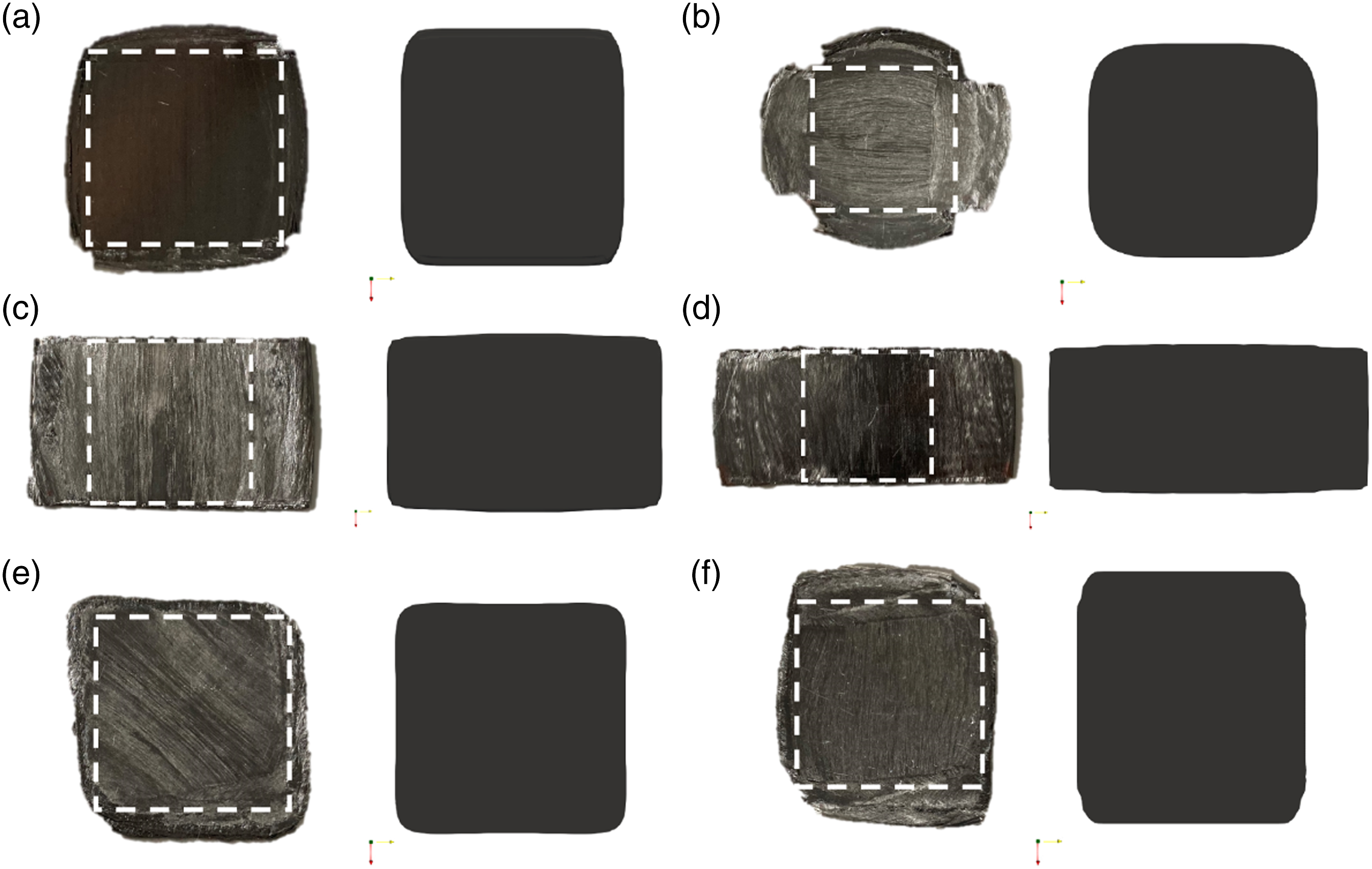

Discussion

In this work, experiments were performed to capture the anisotropic squeeze flow two-dimensionally for different layups and two specimen sizes by recording the material behavior during the heating and cooling phases in a laboratory-scale consolidation unit and quantifying the results using gray scale analysis. The experimental results plotted in Figure 12 highlight the difference in flow behavior between crossply, UD and quasi-isotropic layups. It also shows that the 30 × 30 mm² specimens were squeezed more than the 40 × 40 mm² specimens, which resulted from a higher pressure acting on the specimen due to the smaller area, as the set pressure of the heating press, which acts on the pneumatic piston, was kept constant for all specimens. The experiments in which a temperature sensor was implemented in the specimen show that, as cooling was rapid, the material solidified, and thus the cooling press had no influence on the squeezing. In some cases, the standard deviation was high, which may be due to inaccurate specimen geometries and errors in the video analysis.

The model presented allows the flow behavior to be described as a function of the layup design. Since comparison between experiment and simulation in terms of temperature at the core of the specimen showed good agreement, it can be assumed that the thermodynamic model is adequate. While in some cases the simulation was terminated prematurely due to numerical instabilities, the overall deviation from the experiments was between 2.99% and 26.93% over the entire simulation time and between 0.74% and 48.19% for the last data point of the simulation.

Since the case of UD layups is a mathematical extreme for the model, volume continuity was violated at some point and the simulation terminated. The model requires a ratio of fiber length to diameter for an entire layer, but the choice of this value proved difficult for ± 45° fiber direction layups because fiber length varies over the area. For these cases, an average value was chosen, which may have led to deviations of the flow behavior from reality. Consequently, the qualitative comparison also shows differences in the final consolidated part, especially in the corners, where the fiber length is in reality much shorter than in the center of the area, which is not considered in the simulation. For these reasons, it is clear why the best results were obtained for the “Crossply90” layups.

Summary and outlook

We have presented a modeling strategy for the anisotropic squeeze flow during hot-press consolidation as a function of fiber orientation and temperature-dependent material properties. The thermodynamic behavior was modeled and validated by means of three layup configurations. The approach presented by Rogers ²² was adapted and implemented in a previously presented solver ⁶ developed for the CFD tool OpenFOAM^®. To validate the model, experiments with various fiber orientations and specimen sizes were performed and compared. The greatest deviations in the changes in length and thickness were between 0.74% and 48.19%, while the overall average deviation for all simulations performed was 7.17%.

The model has shown limitations due to numerical instabilities for some of the cases considered and inaccuracies related to the choice of the aspect ratio of the fiber, which must be set as a constant for each layer. In reality, however, this is not the case when fiber directions of ± 45° are used. Acceptable results were achieved nonetheless when a mean value over the area was set. Further, the change in fiber direction caused by squeeze flow, as apparent in some samples in Figure 17, was ignored in this work, but may lead to increased deviations of the simulation from the experiment.

Since this study focused exclusively on the influence of fiber orientation on the squeeze flow behavior, we plan to additionally consider different process settings as part of future work. To this end, observations at higher cooling-press temperatures will be made to avoid premature solidification of the material.

In general, squeeze flow should be avoided because it can cause significant changes in the geometry of a part, which is usually undesirable. It can also lead to internal stresses and distortion. With the presented simulation, extensive squeeze flow and unwanted changes in part thickness and length or width can be predicted and prevented in production processes.

The bonding behavior during consolidation and the balance between extensive squeeze flow and sufficient bonding were outside the scope of this work, but are further important issues to be investigated in the future. In addition, the applicability of the presented simulation to an industrial scale consolidation process needs to be evaluated.

The presented model assumes an incompressible material behavior. However, Tierney and Gillespie^30,31 showed that the presence of voids in thermoplastic tapes might strongly disallow the assumption of an incompressible material. In future work, the void content of the income material, which in this work is UD tapes, and its effect on the material behavior during consolidation needs to be investigated to verify if the assumption of incompressibility can be made.

Lastly, it should also be noted that no attention was paid to simulation time or its optimization, i.e. no symmetry planes were used, which can significantly reduce the simulation time.