Dynamic mechanical analysis of PA 6 under hydrothermal influences and viscoelastic material modeling

Abstract

Polyamides serve as matrix material for fiber reinforced composites and are widely applied in many different engineering applications. In this context, they are exposed to various environmental influences ranging from temperature to humidity. Thus, the influence of these environmental conditions on the mechanical behavior and the associated implications on the performance of the material is of utmost importance. In this work, the thermoviscoelastic behavior of polyamide 6 (PA 6) for two equilibrium moisture contents is investigated. To this end, dynamic mechanical analysis tests with and without humidity control of the environmental chamber were performed. In terms of relaxation tests, the experimental results reveal drying effects and increased diffusion activities when the sample’s equilibrium moisture content differs from the ambient humidity level within the testing chamber. Temperature-frequency tests quantify the humidity-induced shift of the glass transition temperature. The linear generalized Maxwell model (GMM) and time-temperature superposition are used to analyze the hydrothermal effects on the linear viscoelastic material properties and the onset of mechanical nonlinearity. Based on these investigations and findings, insight is gained on the humidity influence on the material properties and the limitations of linear thermoviscoelastic modeling. Furthermore, the computational construction of master curves and the parameter identification for a generalized Maxwell model are described in detail.

Introduction

Polymer-based materials are widely used in many engineering fields ranging from the automotive sector to naval applications. As basis for fiber reinforced composites,^1,2 they contribute to high-performance structures while enabling cost-efficient production. ³ There is a large number of polymer matrices in use, which differ greatly in their physical properties. Polyamides in particular have proven their worth as polymeric matrix materials and are increasingly applied due to their outstanding specific mechanical and thermal properties as well as chemical resistances. However, during service, the polymer material may be exposed to harsh environments that limits its use. Due to the hydrophilic nature of the amide functional groups of polyamides, the relative humidity strongly influences the performance of the material which leads to a major challenge in technical applications. ⁴ In addition to the hygroscopic behavior, the time-, temperature-, and frequency-dependent behavior needs also to be accounted for the viscoelastic material modeling.^5,6

Viscoelastic material modeling of polyamide 6

Detailed overviews on linear viscoelastic modeling can be found in.^7–9 The basic integral formulation of linear viscoelasticity is given by the Boltzmann superposition integral. Schapery ¹⁰ extended this integral expression to model nonlinear viscoelastic behavior of polymers.

In differential formulations, rheological elements are used.^7,9 The basic elements are linear springs and linear dashpots associated with stiffnesses and relaxation (retardation) times, respectively. These elements can be combined to more complex models. The generalized Maxwell model (GMM) and the generalized Kelvin model are often used to model the viscoelastic behavior of polymers. ¹¹ These models are used for strain driven and stress driven processes, respectively. Both models are equivalent and the relations between the models are well known.^11,12 These differential models can be reformulated yielding the Boltzmann superposition integral where the kernel function is given by the so called Prony series. Kießling and Ihlemann ¹³ used the GMM to model the viscoelastic behavior of PA 6 in the context of large deformations. Koyanagi et al. ¹⁴ developed a viscoelastic-viscoplastic material model for PA 6 where a GMM was considered for the viscoelastic part. Under special assumptions, a differential formulation of the nonlinear Schapery model exists.^15,16 In three-dimensional and isotropic formulations of the linear viscoelastic models, a decomposition into spherical and deviatoric parts is used.^12,17,18

Time-temperature superposition principle

A common approach to model temperature-dependent behavior in the linear viscoelastic regime is to assume thermorheological simplicity.^7,8 For a GMM with multiple elements, the stiffnesses are independent of temperature whereas relaxation (retardation) times depend on temperature by the same function. ¹⁹ In the Boltzmann superposition integral, a reduced time scale is introduced.^7,20

For isothermal processes, time-temperature superposition (TTS) arises. On a logarithmic scale, viscoelastic properties at various temperatures can be derived by temperature-dependent time (frequency) shifts.^7,19 Experimental measurements at various temperature levels can be combined to master curves with a larger time (frequency) range.^21–23

The Williams-Landel-Ferry (WLF) equation ²⁴ and the Arrhenius equation are often used to describe the shift function.^25–27 The WLF equation is based on the concept of changes in free volume and is mainly applicable for temperatures above the glass transition temperature θ_g. The Arrhenius equation is often used for temperatures lower than θ_g. Other approaches for shift functions are given by Kristiawan et al. ²⁸ and Shangguan et al. ²⁹

Thermorheological simplicity can be checked by so called Cole-Cole plots ³⁰ or van Gurp plots.^31–33 In this context, the viscoelastic properties measured by dynamic mechanical analysis (DMA) in temperature-frequency sweeps are used as input. In Cole-Cole plots, the loss modulus is then plotted over the storage modulus. In van Gurp plots, the loss factor is plotted over the dynamic modulus. If thermorheological simplicity is valid, smooth curves result.

If TTS is not applicable, the material behaves thermorheological complex, e.g., in terms of temperature-dependent moduli. This can be modeled by adding a vertical shift.^31,34 A formula for the vertical shift depending on temperature and density can be derived by the Rouse model.^19,35 Brinson and Brinson ⁷ show that the neglection of vertical shifts can cause large errors in the master curves.

Similar to TTS, other influences like moisture content and load level can also be modeled by shift functions. The influence of water on the material properties of polyamides has been widely studied. In this context, time-moisture content superposition plays an important role.^36–38 Ishisaka and Kawagoe ³⁹ investigated the time-moisture content superposition of PA 6 and epoxy resin based on temperature-frequency tests at different relative humidity levels. In terms of PA 6, the relationship for time-moisture content superposition followed a WLF-type equation. Walter et al. ⁴⁰ modeled the influence of moisture concentration by a moisture-dependent reference temperature within the WLF equation.

Ferry and Stratton ⁴¹ used the concept of changes in the free volume to derive an approach for the dependence of the shift factor on temperature, moisture, and load.^42,43 Many authors use the resulting shift function to apply time-temperature-stress superposition.^44–46 Hadid et al. ⁴⁷ applied time-stress superposition to multi-step creep tests of PA 6.

Humidity influence on polyamides

In recent years, many different aspects of moisture absorption in PA 6 have been investigated. Among them, for example, the volume and associated geometry change during water absorption. ⁴⁸ Since the absorbed water acts as a plasticizer, ⁴⁹ this leads to a change in the mechanical properties, such as in the glass transition temperature. ⁵⁰ The amorphous phase of polymers can shift from glassy to rubbery state with water uptake leading to a shift of up towards 60–70  K of the glass transition temperature to lower temperatures. ⁴ First approaches to predict the glass transition temperature as a function of water uptake were developed by Kelley and Bueche ⁵¹ and Reimschuessel. ⁵²

However, not only the influence of moisture on the thermoviscomechanical properties is of utmost importance but also the inducing mechanisms. In this context, many authors focused on the investigation and modeling of diffusive processes.^53–55 According to Alfrey et al., ⁵⁶ diffusion in polymers can be classified by three classes: Fickian (or Case I), non-Fickian (or anomalous), and Case II diffusion. In terms of Fickian diffusion, the rate of diffusion is smaller compared to the rate of relaxation, whereas for Case II the diffusion is much faster than the relaxation. Non-Fickian diffusion is characterized by comparable diffusion and relaxation rates. The mass uptake absorbed at time t can be described by two constants, K and n, reading M(t) = Kt ⁿ . In terms of Fickian diffusion, the exponent n reads 1/2. Case II diffusion is characterized by n = 1 and non-Fickian diffusion by 1/2 < n < 1, cf. ⁵⁶ Nowadays, Case II diffusion is considered as non-Fickian diffusion, such that, generally, one distinguishes between diffusive processes that either obey Fick’s law or are described by a non-Fickian diffusion model.

In a semi-crystalline thermoplastic, water plasticizes in amorphous regions between crystalline domains with increased chain mobility.^4,54,57 The Fickian diffusion model (Fick’s second law of diffusion) represents the simplest approach to describe the diffusion in or out of the polyamide material. In this context, the temperature dependence of the diffusion coefficient is often described by an Arrhenius equation.^53,54,58 However, for some polyamides, or especially in the glassy state, Fick’s law is not applicable. ⁵⁹ According to the findings of Arhant et al., ⁶⁰ the kinetics of the diffusion coefficient in the glassy state (below glass transition temperature) can still be well described by a classical Arrhenius-type equation where the diffusion coefficient depends only on the temperature. In the rubbery state (above glass transition), however, the diffusion coefficient appears to be a function of both temperature and water content which can be captured by the free volume theory.

A detailed overview on the effect of water on polyamides is presented in the review article by Venoor et al. ⁶¹

Sharma et al. ⁶² developed a finite element model to couple the nonlinear diffusion with viscoelastic material behavior. They simulated the effect of local moisture content on the stiffness of PA 6. A coupling of moisture transport to loading based on a nonlinear diffusion model combined with a linear viscoelastic model is presented in Sharma and Diebels. ⁶³

Sambale et al.^64,65 investigated the moisture gradient effects on the local material properties based on StepScan DSC measurements and low-energy computer tomography techniques combined with finite element simulations. ⁶⁶

Lion and Johlitz ⁵⁵ presented a thermodynamically consistent approach to model the diffusion of fluids or gases into deformable solids. In this context, the fluid-induced changes in the material properties of the solid are considered. An approach to model the properties of polymers under hydrothermal conditions close to the glass transition temperature is presented by Engelhard and Lion. ⁶⁷

In the context of a nonlinear material model at finite strains, the influence of temperature and moisture content on the viscoelastic material properties of PA 6 was investigated by Kießling and Ihlemann. ¹³

Since the influence of water plays an important role when dealing with polyamides, guidelines for sample preparation, ⁶⁸ conditioning programs,^49,69,70 and experimental treatment were developed. ⁷¹

Motivation and outline

The present work is motivated by the preliminary work on nonlinear viscoelasticity. ¹⁶ The overall objective is to develop a nonlinear viscoelastic material model that accounts additionally for hydrothermal influences based on the respective experimental investigations. In this work, however, focus is set on linear viscoelastic modeling and experimental investigations for hydrothermal conditions. The influence of humidity control and no humidity control during a static and dynamic test is discussed. In literature, many experimental investigations of polyamides at different distinct humidity levels are documented. Here, additionally, the influence of humidity during the measurement is observed. Furthermore, implications of the humidity content on the linear-nonlinear transition are addressed. The time-temperature superposition principle is investigated under different humidity levels and correlated with its intrinsic properties, i.e. the glass transition temperature θ_g. Furthermore, some limits of the time-temperature superposition principle are identified. Moreover, a numerical shift algorithm for both vertical and horizontal shifting of the dynamic data to obtain master curves is presented.

The outline of the present work is as follows. First, the mechanical fundamentals as well as the fundamental equations for the thermoviscoelastic characterization by means of dynamic mechanical analysis (DMA) are summarized. The test parameters and sample preparation are presented. Moreover, an enhanced method to automatically evaluate the master curves from temperature-frequency tests based on vertical and horizontal shifting of the data is documented. The experimental results from relaxation, temperature-frequency, and humidity sweep tests are presented and discussed. For the temperature-frequency sweeps, the master curves are determined and presented followed by a discussion on the parameter identification for a generalized Maxwell model by least squares optimization. A summary of the main results and concluding remarks are given in the last section.

Fundamentals

Dynamic mechanical analysis

The thermoviscoelastic material behavior can be characterized by means of dynamic mechanical analysis (DMA). In this context, a distinction is generally made between tests with dynamic and static loads. The tests performed for this work are conducted using the testing device GABO Eplexor^®500N^∗ without humidity control and GABO Eplexor^®150N^† with the humidity generator Hygromator^®. The fundamental equations and principle is shortly summarized in what follows. A detailed overview on DMA is given in Menard. ⁷²

Static tests

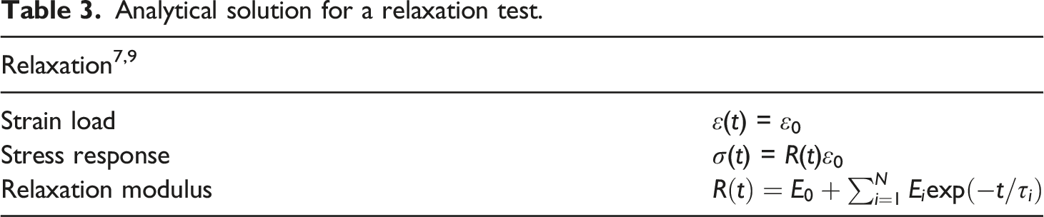
In order to measure the viscoelastic material properties, relaxation tests are performed. Herein, a sample is loaded by a constant strain ɛ₀ and the material’s response is measured resulting in the uniaxial stress-strain response σ(t) = R(t)ɛ₀. ⁷

Dynamic tests

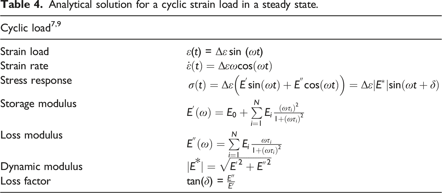
A sample is subjected to a cyclic strain or stress load. For dynamic mechanical analysis, this load contains a static preload ɛ_stat = ɛ₀ which is superimposed by a sinusoidal oscillation ɛ_dyn = Δɛ sin (ωt), with Δɛ denoting the amplitude, and ω the oscillation frequency of the cyclic load, reading

$\epsilon \left(t\right)={\epsilon }_{\text{stat}}+{\epsilon }_{\text{dyn}}={\epsilon }_0+\mathrm{\Delta }\epsilon \sin \left(\omega t\right)$

(1)

During the test, the amplitude of the sample’s deformation as well as the phase shift δ between the cyclic load and the material’s response is measured, yielding

$\sigma \left(t\right)={\sigma }_0+\mathrm{\Delta }\sigma \sin \left(\omega t+\delta \right)$

(2)

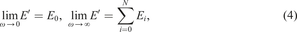
Based on the excitation and the material’s response, the storage modulus E′, representing the instantaneous elastic material response to the oscillation, and the loss modulus E′′, representing the viscous behavior induced by internal friction, for instance, can be determined

$E^{\prime }=\frac{\mathrm{\Delta }\sigma }{\mathrm{\Delta }\epsilon }\cos \left(\delta \right), E^{\prime \prime }=\frac{\mathrm{\Delta }\sigma }{\mathrm{\Delta }\epsilon }\sin \left(\delta \right)$

(3)

The ratio of loss and storage modulus yields the loss factor tan δ. The thermoviscoelastic material properties can be determined by applying varying temperature and frequency loads to the sample.

Sample preparation

Within this work, two differently conditioned sample states are of interest: dry-as-molded (DAM), and ATM-23/50 conditioned samples. The DAM state is defined by a nominal equilibrium moisture content of less than 0.3wt.%. ⁷³ This state is usually present directly after the manufacturing process and can be maintained by storing samples either in a desiccator or in sealed vacuum bags. ⁴⁹ In this work, the samples are re-dried in a vacuum oven and stored afterwards in a desiccator.

Additionally, a conditioned state of the samples is of interest for some industrial applications. In this context, conditioning is performed in order to obtain a specific absorption level of water. ⁷⁴ With respect to polymers, standard atmospheres are defined depending on the application and the polymer considered. The standard atmosphere represents average, non-tropical, laboratory conditions at an equilibrium moisture content between 2.5wt.% and 3.0 wt.%. ⁶ This state can be accomplished by using a climatic chamber and conditioning programs. In ISO 291, ⁶⁹ a procedure is described for the standard atmosphere ATM-23/50, i.e. 23°C and 50%RH. However, the ATM-23/50 conditioning procedure is not applicable for PA 6 since, depending on the sample’s thickness, the equilibrium moisture content will be achieved after about 1 year (for a 2 mm thickness). In order to overcome this drawback, accelerated conditioning programs have been developed. ⁷⁰ To meet the technical possibilities of the climatic chamber Memmert ICH110 L used for this work, the conditioning program presented in Jiaet al. ⁴⁹ is taken into account resulting in an equilibrium moisture content of the samples as obtained by ATM-23/50 conditioning. In this context, the samples of a thickness of 2 mm are stored in the climatic chamber at 55°C and 50%RH (ATM-55/50) for a minimum of 7 days. After this time, the samples are weighed. An equilibrium moisture content is reached if three consecutive weight measurements show a deviation of less than 0.1%. ⁷⁰ After the equilibrium moisture content is reached, the samples are stored at 23°C and 50%RH (ATM-23/50) until further use.

DMA test parameters

The test parameters for the static tests (relaxation) for ATM-23/50 conditioned samples are listed in Table 1. All samples have the dimensions 83 mm × 10 mm × 2 mm with respect to length, width and thickness. Dynamic tests with varying frequency load and temperature (temperature-frequency tests) are performed for DAM and conditioned (ATM-55/50) samples. The respective testing parameters are given in Table 1 as well.

Table 1.

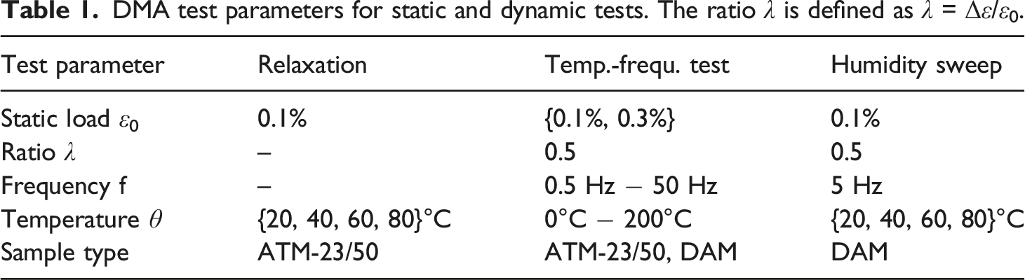
DMA test parameters for static and dynamic tests. The ratio λ is defined as λ = Δɛ/ɛ₀.

Test parameter	Relaxation	Temp.-frequ. test	Humidity sweep
Static load ɛ0	0.1%	{0.1%, 0.3%}	0.1%
Ratio λ	–	0.5	0.5
Frequency f	–	0.5 Hz − 50 Hz	5 Hz
Temperature θ	{20, 40, 60, 80}°C	0°C − 200°C	{20, 40, 60, 80}°C
Sample type	ATM-23/50	ATM-23/50, DAM	DAM

Linear thermoviscoelastic material modeling

Generalized Maxwell model

In this work, the GMM is used to model linear viscoelastic material behavior. As the experimental characterization is performed by uniaxial tests, a one-dimensional model is considered. The model consists of a linear spring with stiffness E₀ and an arbitrary number N of linear Maxwell elements in parallel. Each Maxwell element consists of a linear spring and a linear dashpot in series. The springs and dashpots are characterized by stiffnesses E _i and viscosities η _i , respectively. In Table 2, the main equations for the GMM are summarized. The general solution yields the Boltzmann superposition integral.

Table 2.

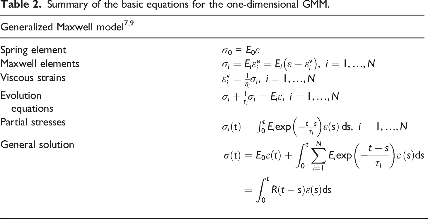
Summary of the basic equations for the one-dimensional GMM.

Generalized Maxwell model7,9
Spring element	σ0 = E0ɛ
Maxwell elements	${\sigma }_i=E_i{\epsilon }_i^{\mathrm{e}}=E_i\left(\epsilon -{\epsilon }_i^{\mathrm{v}}\right), i=1,\dots ,N$
Viscous strains	$\stackrel{.}{{\epsilon }_i^{\mathrm{v}}}=\frac{1}{{\eta }_i}{\sigma }_i, i=1,\dots ,N$
Evolution equations	$\stackrel{.}{{\sigma }_i}+\frac{1}{{\tau }_i}{\sigma }_i=E_i\stackrel{.}{\epsilon }, i=1,\dots ,N$
Partial stresses	${\sigma }_i\left(t\right)={\int }_0^t{E}_i\exp \left(-\frac{t-s}{{\tau }_i}\right)\stackrel{.}{\epsilon }\left(s\right)\hspace{0.17em}\mathrm{d}s, i=1,\dots ,N$
General solution	$\begin{array}{cc}\sigma \left(t\right)=E_0\epsilon \left(t\right)+{\int }_0^t\sum _{i=1}^N{E}_i\exp \left(-\frac{t-s}{{\tau }_i}\right)\stackrel{.}{\epsilon }\left(s\right)\mathrm{d}s& \\ ={\int }_0^{t}R\left(t-s\right)\stackrel{.}{\epsilon }\left(s\right)\mathrm{d}s& \end{array}$

The analytical solution for a relaxation test with constant strain load is shown in Table 3. The analytical solution for a cyclic strain load is summarized in Table 4. The cyclic stress response is given by the storage modulus and loss modulus that describe the elastic and the viscous behavior, respectively. Their asymptotic characteristics are given by

$\begin{array}{cc}\underset{\omega \to 0}{\lim }{E}^{\prime }=E_0, \underset{\omega \to \infty }{\lim }{E}^{\prime }=\sum _{i=0}^N{E}_i,& \end{array}$

(4)

$\begin{array}{cc}\underset{\omega \to 0}{\lim }{E}^{″}=\underset{\omega \to \infty }{\lim }{E}^{″}=0.& \end{array}$

(5)

Table 3.

Analytical solution for a relaxation test.

Relaxation7,9
Strain load	ɛ(t) = ɛ0
Stress response	σ(t) = R(t)ɛ0
Relaxation modulus	$R\left(t\right)=E_0+{\displaystyle \sum }_{i=1}^N{E}_i\exp \left(-t/{\tau }_i\right)$

Table 4.

Analytical solution for a cyclic strain load in a steady state.

Cyclic load7,9
Strain load	ɛ(t) = Δɛ sin (ωt)
Strain rate	$\stackrel{.}{\epsilon }\left(t\right)=\mathrm{\Delta }\epsilon \omega \cos \left(\omega t\right)$
Stress response	$\begin{array}{c}\sigma \left(t\right)=\mathrm{\Delta }\epsilon \left(E^{\prime }\sin \left(\omega t\right)+E^{″}\cos \left(\omega t\right)\right)=\mathrm{\Delta }\epsilon \left|E^{\ast }\right|\sin \left(\omega t+\delta \right)\end{array}$
Storage modulus	$E^{\prime }\left(\omega \right)=E_0+{\displaystyle \sum }_{i=1}^N{E}_i\frac{{\left(\omega {\tau }_i\right)}^2}{1+{\left(\omega {\tau }_i\right)}^2}$
Loss modulus	$E^{″}\left(\omega \right)={\displaystyle \sum }_{i=1}^N{E}_i\frac{\omega {\tau }_i}{1+{\left(\omega {\tau }_i\right)}^2}$
Dynamic modulus	$\left|E^{*}\right|=\sqrt{{E^{\prime }}^2+{E^{″}}^2}$
Loss factor	tan(δ) = $\frac{E″}{E\prime }$

Time-temperature superposition

Horizontal shift

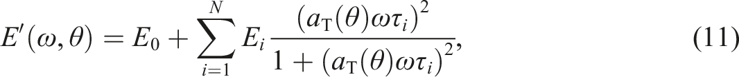
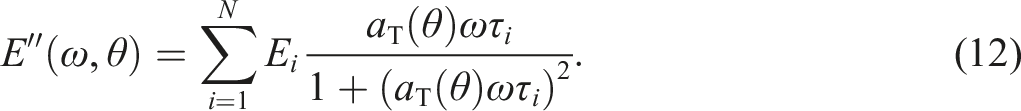
Often, thermorheological simplicity is assumed to model temperature-dependent viscoelastic behavior. This means that all viscosities of the GMM depend on temperature in the same manner. The stiffnesses are independent of temperature. The viscosities, and consequently the relaxation times, are given by

${\eta }_i\left(\theta \right)=a_{\mathrm{T}}\left(\theta \right){\eta }_i^{\text{ref}}, {\tau }_i\left(\theta \right)=a_{\mathrm{T}}\left(\theta \right){\tau }_i^{\text{ref}}, i=1,\dots ,N$

(6)

The temperature-dependent shift function a_T(θ) has the following properties

$a_{\mathrm{T}}\left({\theta }_{\text{ref}}\right)=1, a_{\mathrm{T}}\left(\theta \right)>0, a_{\mathrm{T}}^{\prime }<0.$

(7)

The reference temperature θ_ref can be arbitrarely chosen. The temperature-dependent Boltzmann superposition integral reads

$\sigma \left(t\right)={\int }_0^{t}R\left(z\left(t\right)-u\left(s\right),{\theta }_{\text{ref}}\right)\stackrel{.}{\epsilon }\left(s\right)\mathrm{d}s.$

(8)

In this case, an effective time (reduced time) is defined by^7,20

$z\left(t\right)={\int }_0^t\frac{\mathrm{d}w}{a_{\mathrm{T}}\left(\theta \left(w\right)\right)}, u\left(s\right)={\int }_0^s\frac{\mathrm{d}w}{a_{\mathrm{T}}\left(\theta \left(w\right)\right)}.$

(9)

For θ > θ_ref, the material time is faster than the physical time and vice versa. Assuming isothermal processes, a_T(θ) = const., equation (8) yields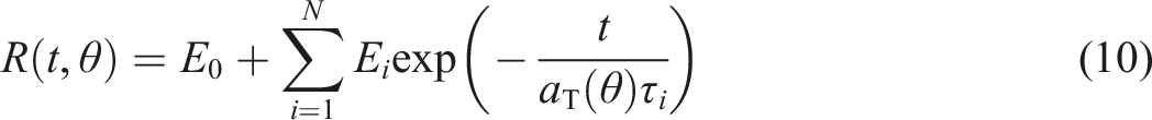

$R\left(t,\theta \right)=E_0+{\displaystyle \sum }_{i=1}^N{E}_i\exp \left(-\frac{t}{a_{\mathrm{T}}\left(\theta \right){\tau }_i}\right)$

(10)

for the relaxation test and

$\begin{array}{cc}{E}^{\prime }(\omega ,\theta )& =E_0+{\displaystyle \sum }_{i=1}^N{E}_i\frac{(a_{\mathrm{T}}(\theta )\omega {\tau }_i{)}^2}{1+(a_{\mathrm{T}}(\theta )\omega {\tau }_i{)}^2},\end{array}$

(11)

$\begin{array}{cc}{E}^{″}\left(\omega ,\theta \right)& ={\displaystyle \sum }_{i=1}^N{E}_i\frac{a_{\mathrm{T}}\left(\theta \right)\omega {\tau }_i}{1+(a_{\mathrm{T}}(\theta )\omega {\tau }_i{)}^2}\end{array}.$

(12)

for the cyclic load case. The expressions t/a_T and ωa_T are called reduced time and reduced frequency, respectively. Then

$\begin{array}{c}R\left(t,\theta \right)=R\left(\frac{t}{a_{\mathrm{T}}},{\theta }_{\text{ref}}\right)=R\left({10}^{\log t-\log \hspace{0.17em}{a}_{\mathrm{T}}},{\theta }_{\text{ref}}\right),\end{array}$

(13)

$\begin{array}{c}{E}^{\left(·\right)}\left(\omega ,\theta \right)=E^{\left(·\right)}\left(\omega a_{\mathrm{T}},{\theta }_{\text{ref}}\right) =E^{\left(·\right)}\left({10}^{\log \omega +\log \hspace{0.17em}{a}_{\mathrm{T}}},{\theta }_{\text{ref}}\right)\end{array},$

(14)

with

$E^{(·)}=E^{\prime },E^{″}$

(15)

holds. A deviation from the reference temperature leads to a time (frequency) shift on logarithmic scale. If time or frequency is plotted on the x-axis, a horizontal shift arises. This principle is called time-temperature superposition.

Vertical shift

Thermorheological simplicity can be extended by using an additional vertical shift.^19,34 By introducing b_T(θ) as vertical shift function, one yields

$E_i\left(\theta \right)=b_{\mathrm{T}}\left(\theta \right)E_i^{\text{ref}}, i=1,\dots ,N.$

(16)

As the shift function is the same for all stiffnesses, equation (10) and (12) are multiplied by this function, reading

$\begin{array}{cc} \stackrel{\sim }{R}\left(t,\theta \right)& =b_{\mathrm{T}}\left(\theta \right)R\left(t,\theta \right),\end{array}$

(17)

$\begin{array}{cc} {\stackrel{\sim }{E}}^{(·)}\left(\omega ,\theta \right)& =b_{\mathrm{T}}\left(\theta \right)E^{(·)}\left(\omega ,\theta \right)\end{array}.$

(18)

On a double-logarithmic scale, this leads to an additional vertical shift

$\begin{array}{cc}\log \stackrel{\sim }{R}\left(t,\theta \right)& =\log b_{\mathrm{T}}\left(\theta \right)+\log R\left(t,\theta \right),\end{array}$

(19)

$\begin{array}{cc}\log {\stackrel{\sim }{E}}^{(·)}\left(\omega ,\theta \right)& =\log b_{\mathrm{T}}\left(\theta \right)+\log E^{(·)}\left(\omega ,\theta \right)\end{array}.$

(20)

Method of normalized arc length minimization

In experimental testing, a limited range of time (frequency) can be considered. TTS enables to combine experimental data at different temperature levels to obtain a single master curve by shifting. Thereby, viscoelastic behavior can be characterized for a larger time (frequency) range. To avoid manual shifting, numerical shift methods can be applied. The methods found in literature can be grouped in four categories. The method developed by Cho ⁷⁵ minimizes the arc length of the master curve to determine shift factors.^75–77 The closed form algorithm gives an analytical formula for the shift by setting the area between neighbouring curves to zero.^78–80 The methods of Alwis and Burgoyne, ²⁵ Honerkamp and Weese, ⁸¹ and Sihn and Tsai ⁸² use a combination of polynomial interpolation and minimization of squared errors. Other methods are based on numerical derivatives of the viscoelastic properties.^83–85 The method used in this work is based on the work by Bae et al. 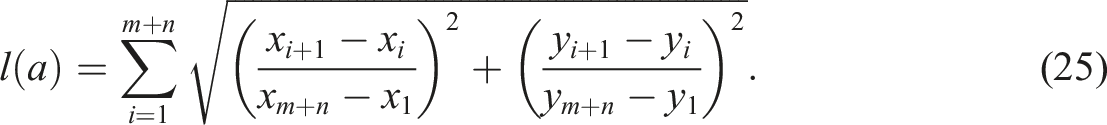⁷⁶ This method is chosen due to its simple implementation and lower requirements to the number of data points. The idea of the method is visualized by Figure 1. In Figure 1(a), two curves are examplarily given. The red curve needs to be shifted and the blue curve serves as reference curve. The shift of the red curve to the final position is shown in Figure 1(b). For an automated method, a quantitative parameter is defined. In this context, the arc length l(a) is introduced as a function of the shift a. The method determines the shift that minimizes the arc length. Therefore, global optimization is used

$l\left(a\right)\to \underset{a\in \left[a_{\mathrm{L}},a_{\mathrm{U}}\right]}{\min }.$

(21)

Figure 1.

Visualization of the shift method: (a) Initial state of the blue and the red curve. (b) The blue curve serves as reference curve and the red curve is shifted by minimizing the normalized arc length.

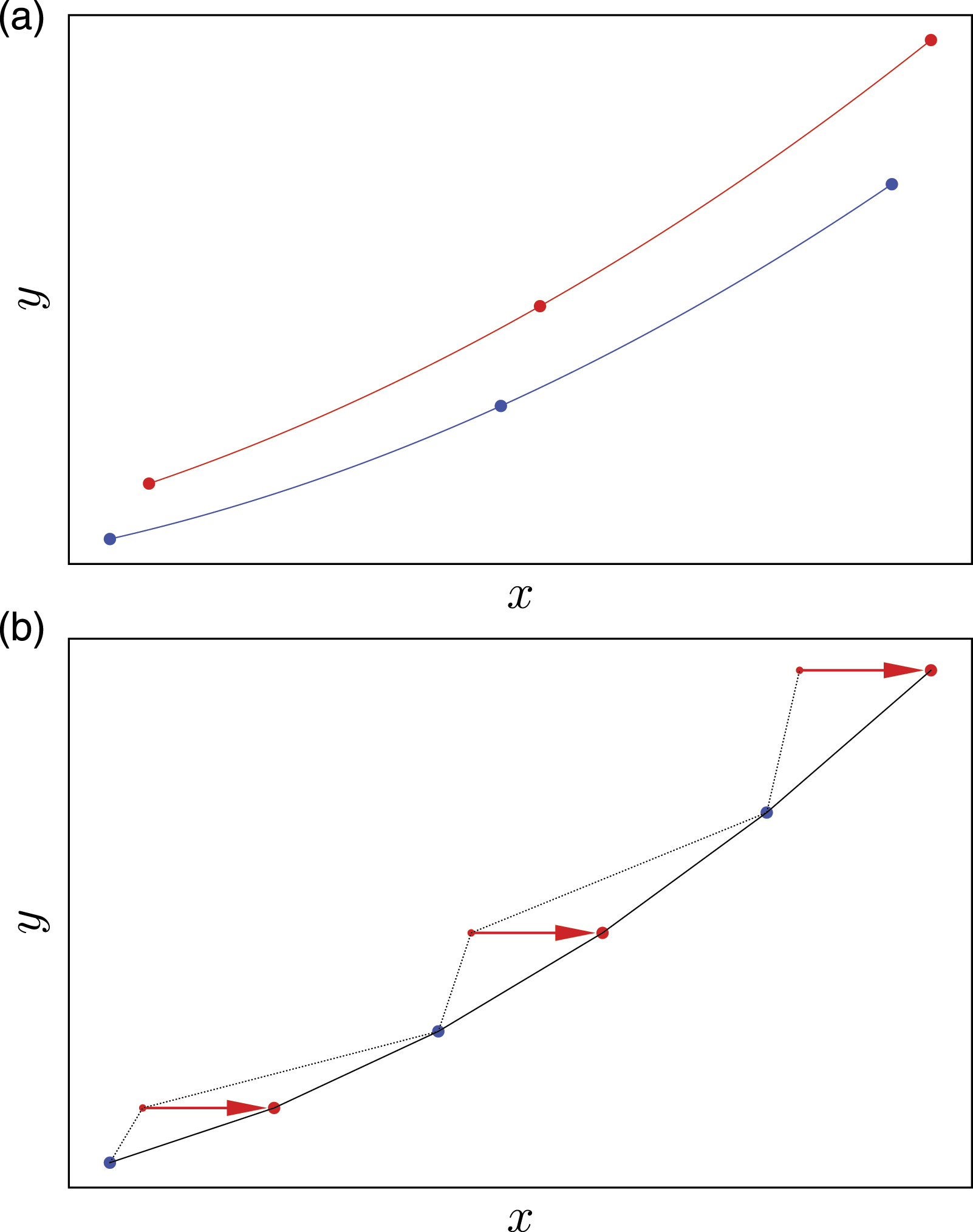
The lower and upper bounds for the shift, a_L, a_U, are prescribed by the user. Each increment of the global optimization scheme, has the following structure

(i) Define the reference curve by L₁ and the shifted curve by L₂

$\begin{array}{cc}{L}_1& =\left\{\left(x_1^{\left(1\right)},y_1^{\left(1\right)}\right),\dots ,\left(x_m^{\left(1\right)},y_m^{\left(1\right)}\right)\right\},\end{array}$

(22)

$\begin{array}{c}{L}_2=\left\{\left(x_1^{\left(2\right)}+a,y_1^{\left(2\right)}\right),\dots ,\left(x_n^{\left(2\right)}+a,y_n^{\left(2\right)}\right)\right\}\end{array}.$

(23)

The number of data points in each list is given by m and n, respectively.

(ii) Combine both lists and sort the resulting list by the x-values in ascending order

$\begin{array}{cc}L=L_1\cup L_2:=\left\{\left(x_1,y_1\right),\dots ,\left(x_{m+n},y_{m+n}\right)\right\}, x_1\le x_2\le \dots \le x_{m+n}.& \end{array}$

(24)

• (iii) Calculate the normalized arc length

$l\left(a\right)={\displaystyle \sum }_{i=1}^{m+n}\sqrt{{\left(\frac{x_{i+1}-x_i}{x_{m+n}-x_1}\right)}^2+{\left(\frac{y_{i+1}-y_i}{y_{m+n}-y_1}\right)}^2}.$

(25)

The method extends the method presented in Bae et al. ⁷⁶ and Cho ⁷⁵ by normalizing the partial arc lengths with the total x- and y-range. Thereby, the increasing x-range due to shifting is taking into account, see Figure 1b. By swapping x- and y-data, the method can also be applied for vertical shifts. Dual Annealing optimization, implemented by the scipy package in Python, is used to solve the minimization problem.

The shift method will be applied to data from temperature-frequency sweeps. The measured tan δ(ω) and E′(ω) curves at various temperature levels serve as input. First, the horizontal shift factor a _T (θ) will be determined by using the loss factor since it is not affected by a vertical shift,^35,76,79 cf. Table 4 and equation (18). Starting from the lowest temperature, the relative shifts between neighboring curves are calculated by the shift method with $a\widehat{=}\log a_{\mathrm{T}}^{\left(\text{rel}\right)}$ , $x\widehat{=}\log \omega$ and $y\widehat{=}\tan \delta$ . The number of temperature levels is denoted by n _θ . The results are given by

$\log a_{\mathrm{T}}^{\left(\text{rel}\right)}\left({\theta }_i\right), {\theta }_i<{\theta }_{i+1}, i=2,\dots ,n_{\theta }.$

(26)

The relative shift at the lowest temperature is set to zero. The total shifts are then calculated by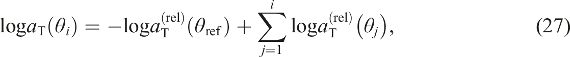

$\log a_{\mathrm{T}}\left({\theta }_i\right)=-\log a_{\mathrm{T}}^{\left(\text{rel}\right)}\left({\theta }_{\text{ref}}\right)+\sum _{j=1}^i\log a_{\mathrm{T}}^{\left(\text{rel}\right)}\left({\theta }_j\right),$

(27)

for i = 1, …, n _θ . The reference temperature can be arbitrarely chosen from θ _i . In a second step, the vertical shift is determined. In this context, the above described procedure is repeated with $a\widehat{=}\log b_{\mathrm{T}}^{\left(\text{ref}\right)}$ , $x\widehat{=}\log E^{\prime }$ and $y\widehat{=}\log \omega$ .

Parameter identification

The last step is to identify parameters for a GMM based on given master curves. This means that a set of 2N + 1 parameters must be identified

${\tilde{\mathcal{P}}}_N=\left\{E_0,E_1,\dots ,E_N,{\tau }_1,\dots ,{\tau }_N\right\}.$

(28)

In general, this is an ill-posed problem as no unique solution exists.^32,86,87 This problem can be solved by prescribing a distribution of relaxation times. ⁸⁸ Jalocha et al. ⁸⁸ developed a method that finds an optimal distribution of relaxation times. In this work, a logarithmic distribution is used.^89,90 Then, only N + 1 stiffnesses need to be identified

${\mathcal{P}}_N=\left\{E_0,E_1,\dots ,E_N\right\}.$

(29)

The number N of Maxwell elements is also prescribed. As a rule of thumb, at least one element per considered frequency decade should be used.^87,91 Least squares minimization is used to solve the problem.^88,89,91 Previously, four viscoelastic properties (E′, E′′, |E*|, tan δ) were introduced for the dynamic load case. Only two of these properties are independent. Here, storage and loss modulus are used as input for the residual.^88,89,91 Formally, the master curves are defined by the data points 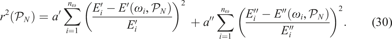$\left\{{\omega }_i,E_i^{\prime }\right\}$ and $\left\{{\omega }_i,E_i^{″}\right\}$ , i = 1, …, n _ω , where n _ω represents the number of data points. The residual is given by

$\begin{array}{l}{r}^2\left({\mathcal{P}}_N\right)=a^{\prime }\sum _{i=1}^{n_{\omega }}{\left(\frac{E_i^{\prime }-E^{\prime }\left({\omega }_i,{\mathcal{P}}_N\right)}{E_i^{\prime }}\right)}^2\\ \end{array}+a^{\prime \prime }\sum _{i=1}^{n_{\omega }}{\left(\frac{E_i^{\prime \prime }-E^{\prime \prime }\left({\omega }_i,{\mathcal{P}}_N\right)}{E_i^{\prime \prime }}\right)}^2.$

(30)

The coefficients a′ and a′′ allow to weight the residuals of storage and loss modulus. ⁹² The constraints

$a^{\prime }+a^{\prime \prime }=1, a^{\prime }>0, a^{\prime \prime }>0$

(31)

are considered. The scipy package in Python is used to determine an optimal stiffness distribution by a gradient-based optimization method (L-BFGS-B). The stiffnesses are forced to be non-negative. The quality of the identification is evaluated by the coefficient of determination (R²-value)

$\begin{array}{c}{R}^2=1-\frac{{\displaystyle \sum }_{i=1}^{n_{\omega }}{\left(E_i^{(·)}-E^{(·)}\left({\omega }_i,{\mathcal{P}}_N^{\text{fit}}\right)\right)}^2}{{\displaystyle \sum }_{i=1}^{n_{\omega }}{\left(E_i^{(·)}-{\overline{E}}^{(·)}\right)}^2},\end{array}$

(32)

$\begin{array}{c}{\overline{E}}^{(·)}=\frac{1}{n_{\omega }}{\displaystyle \sum }_{i=1}^{n_{\omega }}{E}^{(·)}\end{array}.$

(33)

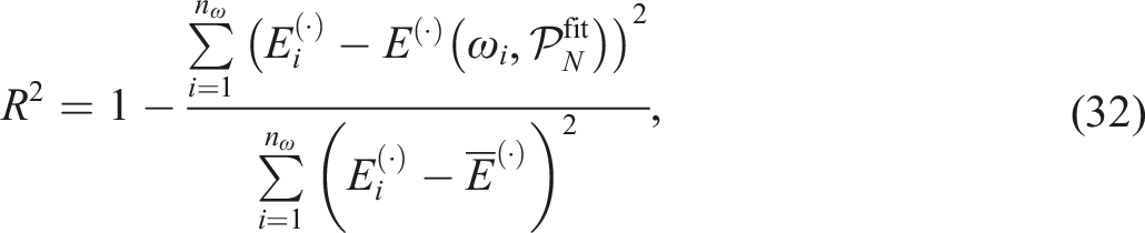
Usually, 0 ≤ R² ≤ 1 holds. The larger the value of R², the better the fit. ⁹³

Experimental investigations

In this section, results are presented focusing on dynamic and static loads and the influence of humidity load on the mechanical properties. Since the material parameters are sensitive to the sample’s moisture content and, thus, the sample’s thickness, ⁶⁴ the respective thickness of the sample used for the experiments is documented in the Appendix. Temperature-frequency tests are performed for ATM-23/50 conditioned PA 6. The experimental data exhibit quantitative evaluation of the viscoelastic properties that serve in what follows as input for the GMM. Relaxation tests indicate not only the viscoelastic behavior but also how diffusive processes during measurement influence the material’s response. Moreover, humidity sweep tests are chosen to show the influence of hydrothermal loads on the mechanical properties.

Relaxation tests

Considering ATM-23/50 conditioned samples, relaxation tests at different temperatures are performed. The test parameters are given in Table 1. The tests for θ = {20, 40, 60, 80}°C are performed with the testing device GABO Eplexor^®500N without humidity control. Thus, the equilibrium moisture content of a sample might, in general, differ from the ambient humidity content within the testing chamber. Additionally, a test at θ = 80°C is repeated with the testing device GABO Eplexor^®150N with the humidity generator Hygromator^®. In this context, the ambient humidity level is set to equal the ATM-23/50 sample’s moisture content of Φ = 50%RH. By this, the difference between humidity control versus no humidity control, i.e. the impact of diffusion, with respect to relaxation tests can be illustrated. In order to exclude influences of the thermal expansion of the crosshead during the measurement, each sample was held at the target temperature for 1  h prior to the relaxation test. After this so-called soak time, the relaxation test was performed. The measurement time presented in this work ranges up to 6  h.

In Figure 2, the experimental results of the relaxation modulus R(t) are depicted. Considering first the data from the tests without humidity control, for all four temperature loads and up to a measurement time of nearly 500 s, R(t), and, thus, σ(t), decreases in a typical manner. However, for t ≥ 500 s and higher temperatures, R(t) increases again after the initial decrease. As the environmental chamber of the DMA testing device exhibits an ambient humidity content of approximately 35%RH, drying of the sample takes place during the test. The chain mobility of polyamides is affected not only by humidity but also by temperature, i.e., the diffusion velocity increases with increasing temperatures. 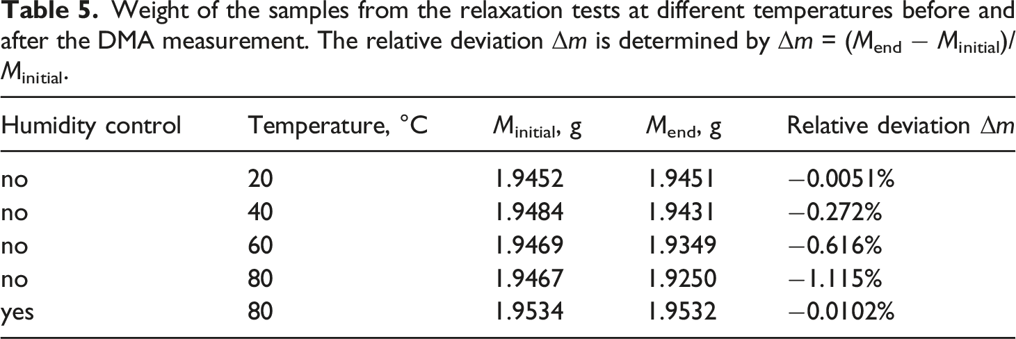⁶¹ Consequently, the diffusion and drying effects are more pronounced for samples at a higher temperature and are detected by an increase of the R(t) curve. Directly before and after the relaxation tests, each sample is weighted. The change in weight is documented in Table 5. For the sample tested at 20°C no significant change in weight is observed, whereas with increasing testing temperature, the samples looses up to 1.115% of weight at 80°C by drying during the measurement. In contrast, considering the experimental results for the test with humidity control ensured by the humidity generator, the relaxation modulus decreases for the total considered time range in a typical manner. Up to 400 s, the curves for θ = 80°C with and without humidity control nearly coincide. However, as the measurement time increases, the curves diverge, highlighting the effects of sample drying and increasing diffusion activities. In many publications, relaxation (or creep) tests are performed for a duration of far less than 400 s. Water sorption during this time does not appear to significantly affect the material behavior, however, for longer periods in the range of hours, a humidity-controlled environmental chamber is meaningful.

Figure 2.

Relaxation modulus depicted over logarithmic time obtained from relaxation tests with ATM-23/50 samples with and without humidity control. HC: humidity control.

Table 5.

Weight of the samples from the relaxation tests at different temperatures before and after the DMA measurement. The relative deviation Δm is determined by Δm = (M_end − M_initial)/M_initial.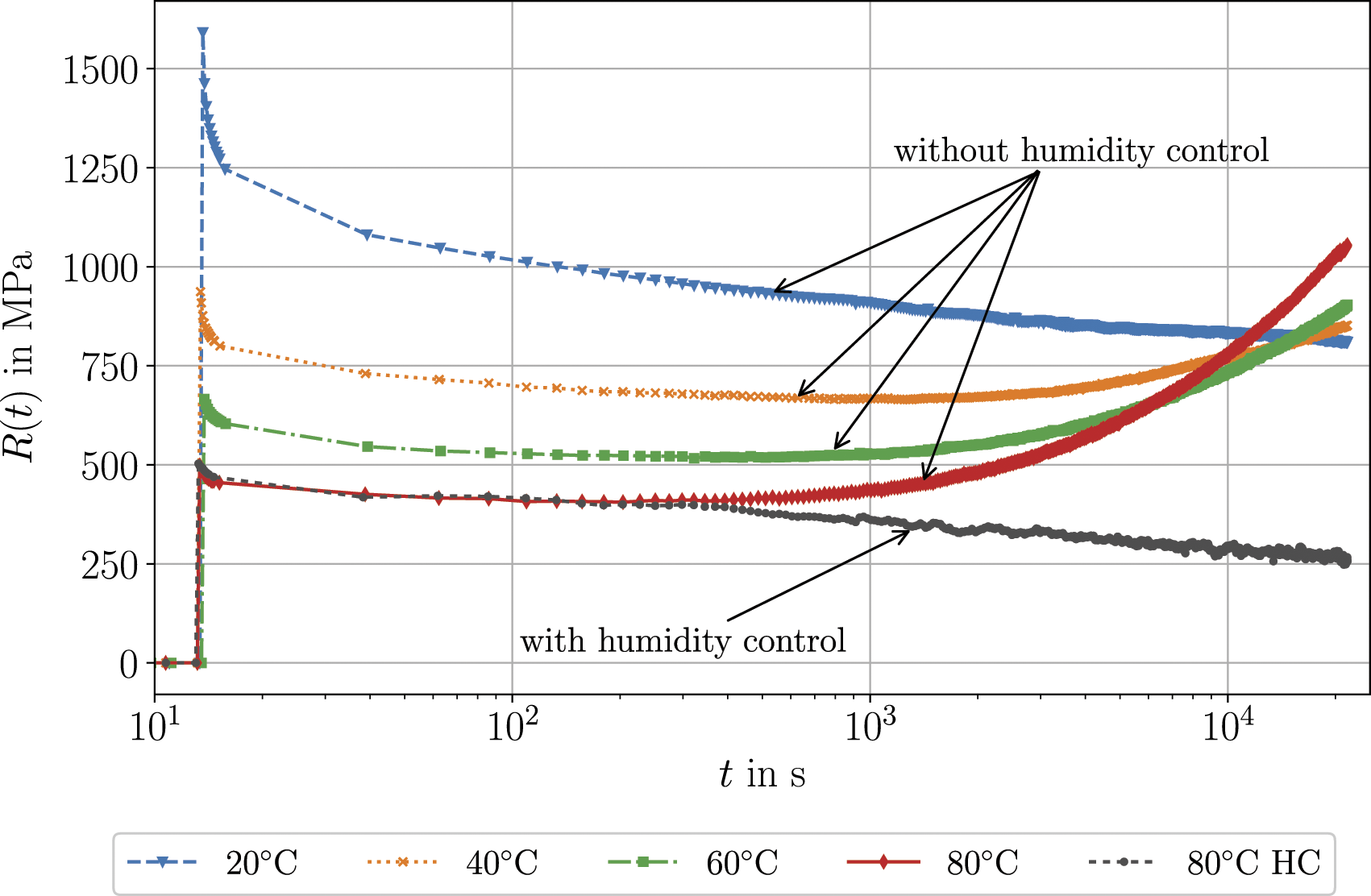

Humidity control	Temperature, °C	Minitial, g	Mend, g	Relative deviation Δm
no	20	1.9452	1.9451	−0.0051%
no	40	1.9484	1.9431	−0.272%
no	60	1.9469	1.9349	−0.616%
no	80	1.9467	1.9250	−1.115%
yes	80	1.9534	1.9532	−0.0102%

Temperature-frequency tests

For a DAM sample, temperature-frequency tests with test parameters according to Table 1 are performed. The results for the storage modulus E′ and the loss factor tan δ over temperature are depicted in Figure 3. The storage modulus shows a highly temperature-dependent behavior, see Figure 3(a), by decreasing strongly with increasing temperature. The decrease from the maximal value of E′ at 0°C to the minimal value at 200°C is about 90%. Within the range 50°C ≤ θ ≤ 100°C, a pronounced dependency on the applied frequency load is shown indicating increasing viscoelastic effects. Generally, E′ exhibits higher values for higher frequency loads throughout the temperature range considered. In Figure 3(b), the loss factor tan δ is depicted over the temperature exhibiting the characteristic shape for polymer-based materials: First, a nonlinear increase of the tan δ curve is shown for increasing temperatures until a peak is reached. After the peak, the curve is decreasing again. There are at least five common methods to determine θ_g as stated in Ehrenstein. ⁹⁴ In this work, the maximum in the loss factor curve is considered to mark the glass transition temperature θ_g. The loss factor exhibits a frequency-dependent behavior, analogously to E′. Considering the lowest and highest frequency load of 0.5 Hz and 50 Hz, respectively, the glass transition temperature θ_g is shifted by 10 K from nearly 70°C to 80°C.

Figure 3.

Temperature frequency tests with DAM sample for 0°C ≤ θ ≤ 200°C and 0.5 Hz ≤ f ≤ 50 Hz. (a) Storage modulus E′ over temperature load revealing thermoviscoelastic material behavior. (b) Loss factor tan δ over temperature indicating frequency-dependent glass transition temperature.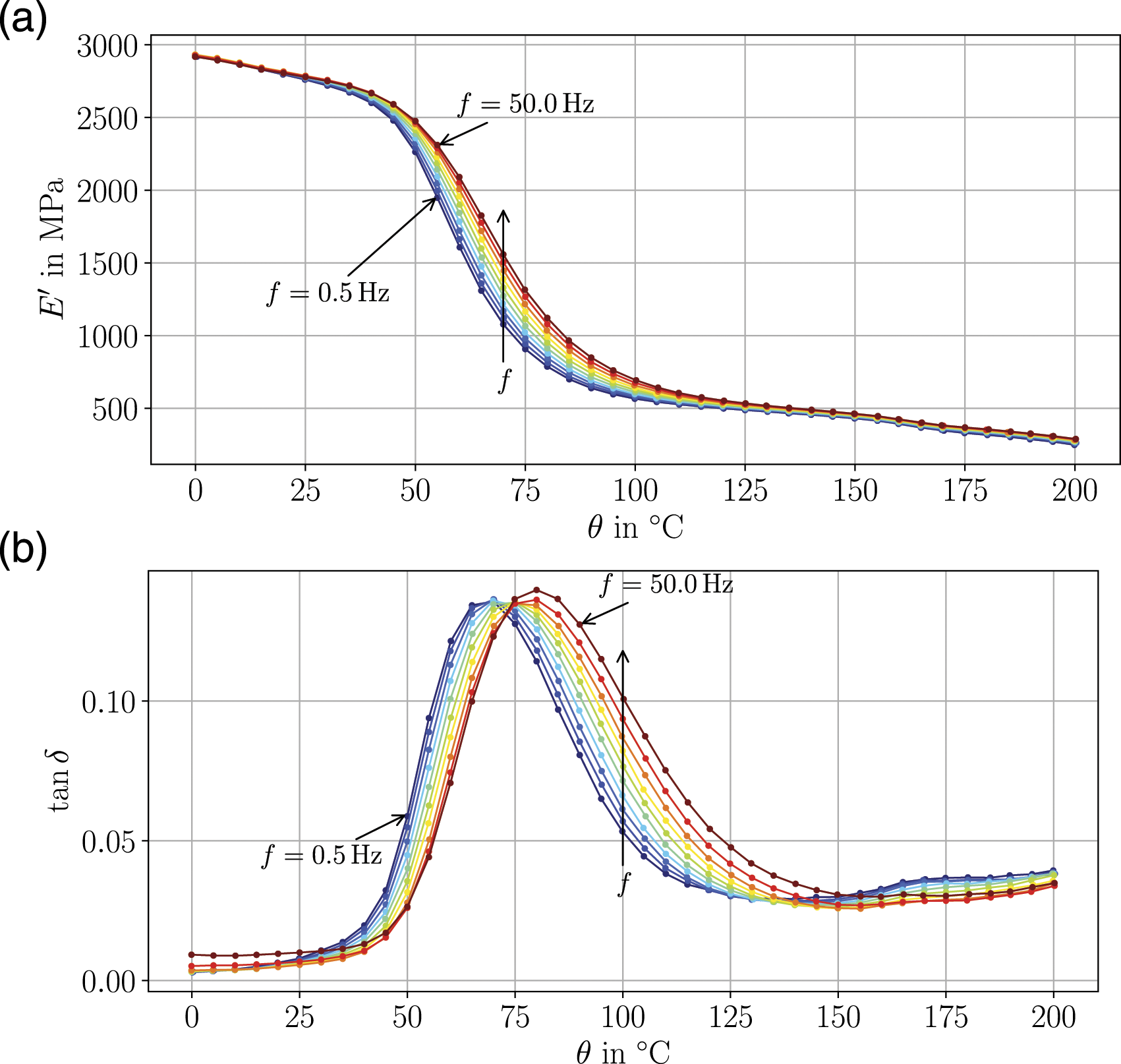

The temperature-frequency test was repeated using a ATM-23/50 conditioned sample. In Figure 4, the experimental data for both ATM-23/50 and DAM samples are depicted for E′ and tan δ considering a frequency load of 5 Hz. The data of the ATM-23/50 samples are shifted towards lower temperatures when compared to the DAM data. The glass transition temperature θ_g is shifted by about −50 K from approximately 75°C (DAM) to 25°C (ATM-23/50). Moreover, the values for tan δ at θ_g are smaller for ATM-23/50 data than for DAM data. The comparison reveals the effect of humidity on the glass transition as reported in literature. ⁶¹

Figure 4.

Comparison of storage modulus E′ and loss factor tan δ over temperature for f = 5 Hz and samples with two different moisture contents (ATM-23/50 and DAM). The higher equilibrium moisture content in the sample shifts the curves and glass transition to lower temperatures.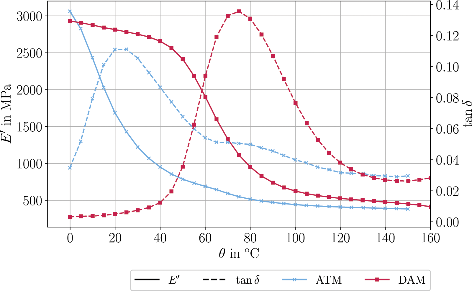

The difference in moisture between a sample and its environment leads to an inhomogeneous moisture content throughout the sample’s thickness and, thus, induces locally varying material properties. A significant moisture gradient throughout the sample’s thickness is reported in Figure 17 of Sharma et al. ⁶² Their simulations reveal that a homogeneous distribution of the moisture content within the sample is reached only after several hours or days, depending on the considered moisture boundary conditions. In Figure 18 of Sharma et al., ⁶² an essential influence of the moisture distribution on the mechanical properties is reported. However, despite the impact of the moisture distribution on the material behavior, they also showed that for loadings in the range of small deformations, ɛ < 0.5%, the heterogeneous moisture distribution has a less significant effect on the overall structural properties, i.e. the effective properties, of the specimen. With respect to the present work, it should be noted that in all tests where ambient humidity is not controlled, a moisture gradient is to be expected within the sample. However, it is assumed that this gradient, especially within the loading regime considered here for the relaxation and temperature-frequency tests, will not significantly affect the measured effective material properties at sample scale. Thus, the experimental results within this work are to be understood as effective properties. Locally distributed material properties due to the possible inhomogeneous moisture distribution are not considered, here.

Humidity sweep

For the investigation of the humidity influence on PA 6, DAM samples are subjected to a dynamic load. Within the environmental chamber, the ambient humidity level varies between 5%RH and 95%RH with a rate of 1%RH/min at a controlled temperature. For temperatures at 20°C, 40°C, 60°C, and 80°C, the storage modulus over the ambient relative humidity content Φ within the environmental chamber is depicted in Figure 5. As illustrated by the graphs in Figure 5, the storage modulus decreases with increasing humidity level. Note that the experimental data obtained from this experiments are not at an equilibrium moisture state but are rather continuously changing. Moreover, due to the continuous change in the humidity level, a gradient of the moisture level within the sample is expected. However, within this work, the data are regarded as effective properties and local inhomogeneities are not taken into account. The effect of gradient moisture distribution on local mechanical properties is discussed in detail by Sambale et al.,^64,65 and on viscoelastic properties by Sharma et al. ⁶²

Figure 5.

Storage modulus E′ over ambient relative humidity content in the environmental chamber at four different temperature loads shows influence of the hydrothermal load on the material’s response. Humidity tests are performed with GABO Eplexor^®150N with the humidity generator Hygromator^®.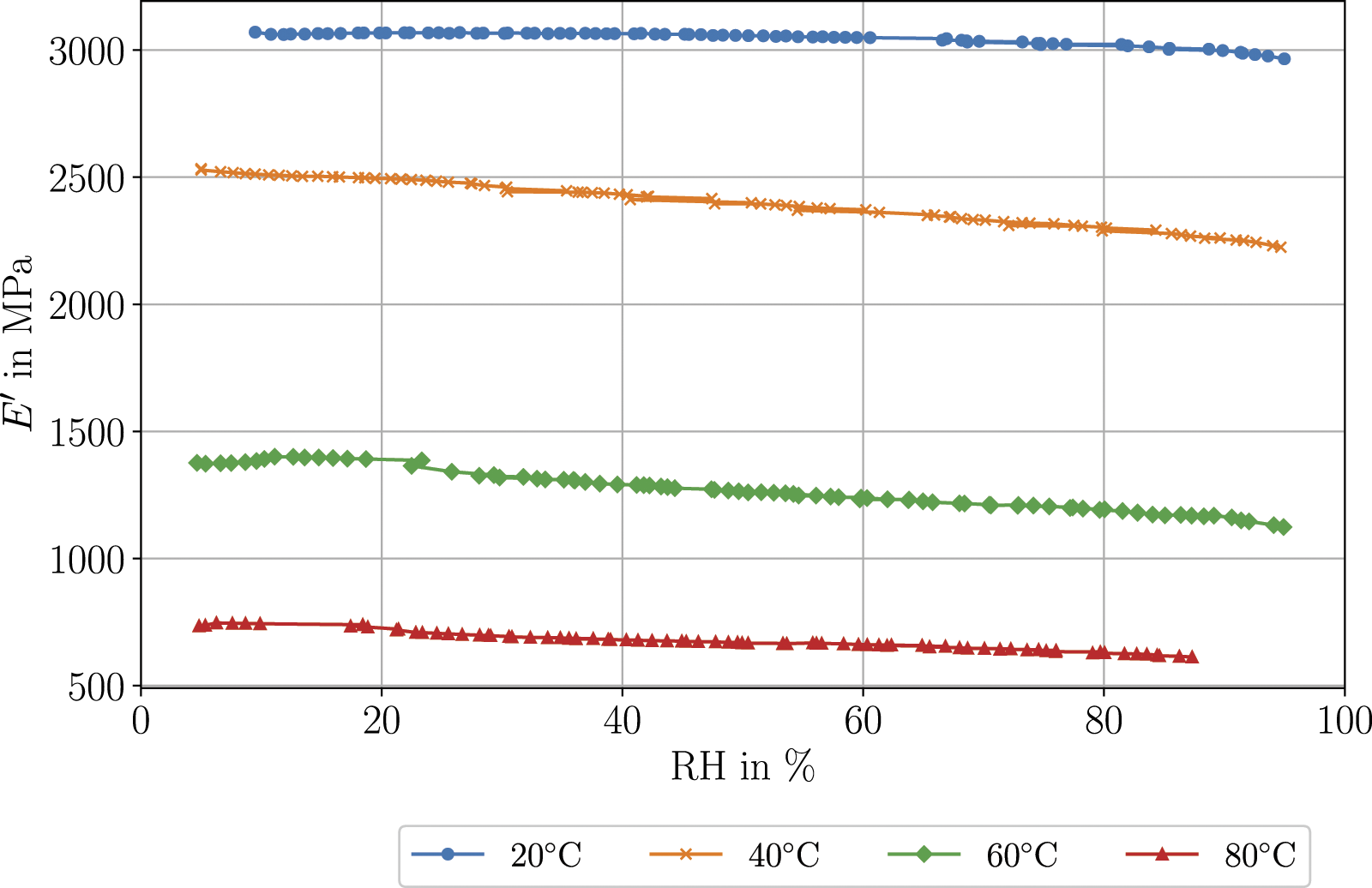

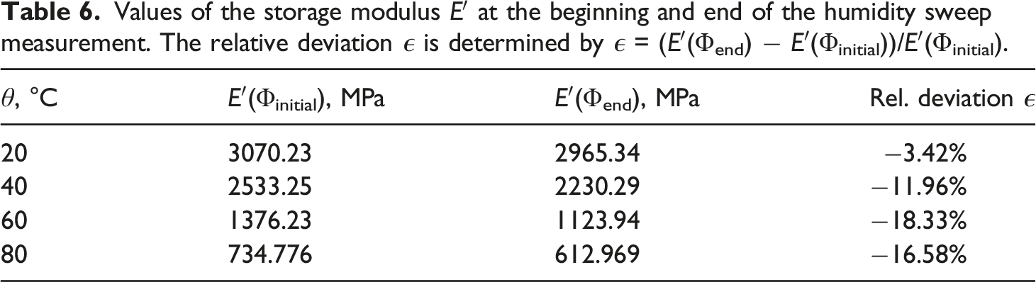
Table 6 lists the quantitative difference between the values of E′ at the beginning and at the end of the measurements for the four different temperatures. At room temperature, the influence of the relative surrounding humidity on the sample appears to be not as significant since here diffusion processes are not within the time scale of the measurement. However, with increasing temperatures, the relative deviation between the initial and final value of E′ increases indicating a strong influence of the humidity on the mechanical behavior at temperatures around θ_g. Since for 80°C the humidity level of 95%RH could not be reached, the relative deviation is in this case smaller than for 60°C but is expected to be in the same range. When comparing the difference in E′ for humidity load and thermal load, the influence of temperature appears as more significant since the drop in E′ is about 76% considering exemplarily Φ = 20%RH and the experimental data for 20°C and 80°C.

Table 6.

Values of the storage modulus E′ at the beginning and end of the humidity sweep measurement. The relative deviation ϵ is determined by ϵ = (E′(Φ_end) − E′(Φ_initial))/E′(Φ_initial).

θ, °C	E′(Φinitial), MPa	E′(Φend), MPa	Rel. deviation ϵ
20	3070.23	2965.34	−3.42%
40	2533.25	2230.29	−11.96%
60	1376.23	1123.94	−18.33%
80	734.776	612.969	−16.58%

Simulation results

Master curve construction

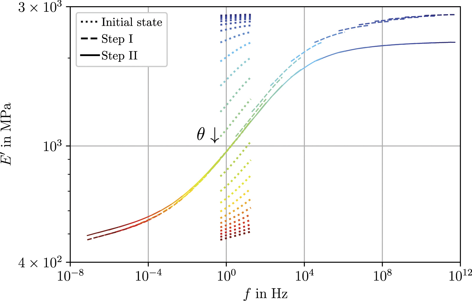
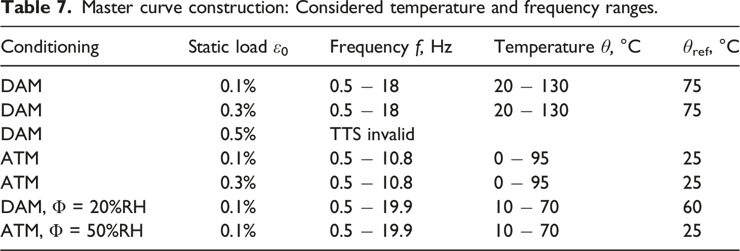
The validity of TTS is checked by Cole-Cole plots and shown for DAM samples in the Appendix. The next step is to construct the master curves by the method described previously. Figures 6 and 7 exemplarily show the shift procedure for a temperature-frequency sweep. The reference temperature is set to θ_g = 75°C. In Figure 6, the horizontal shifting (step I) is illustrated. In the initial state, the individual curves for various temperature levels can be seen. These curves are shifted horizontally. Then, the plot of the loss factor shows a smooth master curve. At reference temperature, both curves coincide. The highest temperature level (130°C) is at the left end, the lowest level (20°C) at the right end. In Figure 7, it can be seen that after step I the plot of the storage modulus is still not smooth. Thus, vertical shifting (step II) is necessary and results in a smooth master curve. The loss factor is not influenced by step II. In Table 7, the considered frequency and temperature ranges for each test are shown. Additionally, the corresponding reference temperature is listed. In all cases, the highest frequency levels are neglected to obtain smooth master curves. Thus, TTS is limited to a physical frequency lower than 20 Hz. This does not contradict the plots in Figures 6 and 7 since these plots include frequencies above the limit of 20 Hz in the sense of reduced frequencies. With increasing moisture, the temperature range, in which TTS is applicable, is shifted to lower temperatures. This can be seen by comparing DAM and ATM samples. For ɛ₀ ≤ 0.3%, TTS is valid and the limitations in temperature and frequency range are not affected by the load level.

Figure 6.

Horizontal shifting is applied to loss factor data. The dotted lines show the unshifted data at various temperatures. The solid lines represent the horizontally shifted data. From the blue to the red lines, temperature is increasing. The reference temperature is 75°C.

Figure 7.

Horizontal and vertical shifting is applied to storage modulus data. The dotted lines show the input data. The dashed lines result after horizontal shifting. Adding vertical shifts leads to the solid lines. The reference temperature is 75°C.

Table 7.

Master curve construction: Considered temperature and frequency ranges.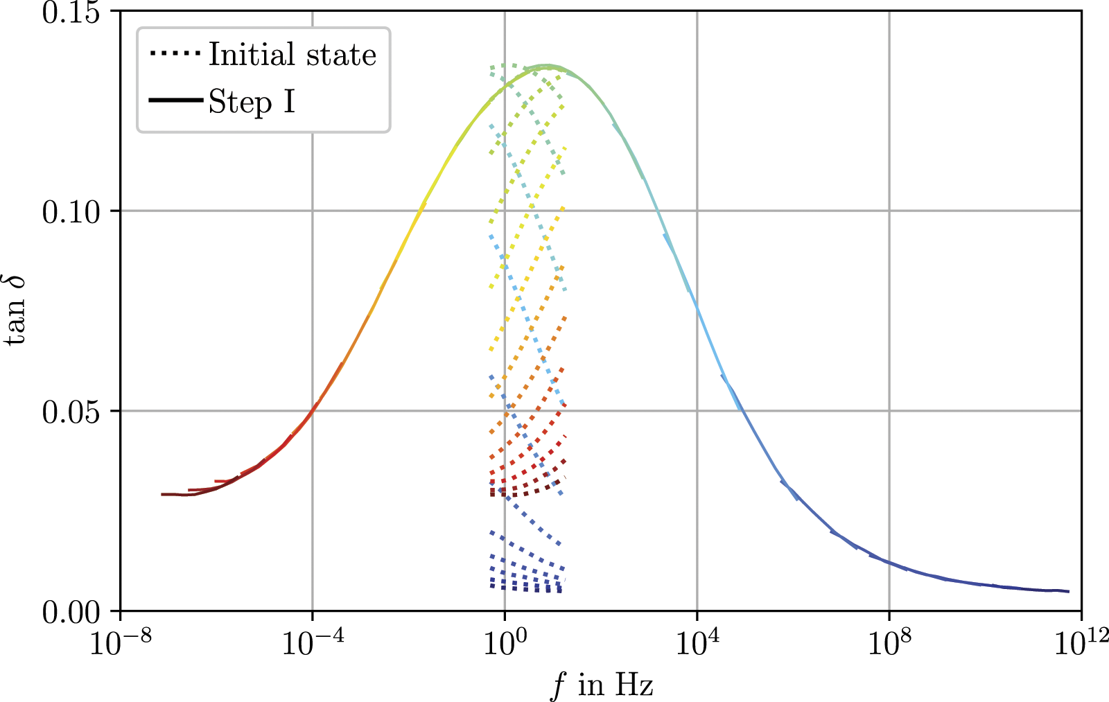

Conditioning	Static load ɛ0	Frequency f, Hz	Temperature θ, °C	θref, °C
DAM	0.1%	0.5 − 18	20 − 130	75
DAM	0.3%	0.5 − 18	20 − 130	75
DAM	0.5%	TTS invalid
ATM	0.1%	0.5 − 10.8	0 − 95	25
ATM	0.3%	0.5 − 10.8	0 − 95	25
DAM, Φ = 20%RH	0.1%	0.5 − 19.9	10 − 70	60
ATM, Φ = 50%RH	0.1%	0.5 − 19.9	10 − 70	25

Comparison of different master curves

In Figures 8 and 9, master curves obtained from dynamic tests are shown. Storage modulus and loss modulus are plotted on a double-logarithmic scale. The reference temperature is set to the corresponding approximated glass transition temperature for each curve, θ_ref = 75°C for DAM samples without humidity control, θ_ref = 60°C for DAM samples with humidity control, and θ_ref = 25°C for ATM samples.

Figure 8.

Master curves for ATM-23/50 (θ_ref = 25°C) and DAM samples (θ_ref = 75°C) obtained from temperature-frequency tests at mean strains of 0.1% and 0.3% without humidity control.

Figure 9.

Master curves obtained from temperature-frequency tests at mean strains of 0.1% with humidity control. Tests were performed with an ATM-23/50 conditioned sample at 50%RH (θ_ref = 25°C) and with a DAM sample at 20%RH (θ_ref = 60°C).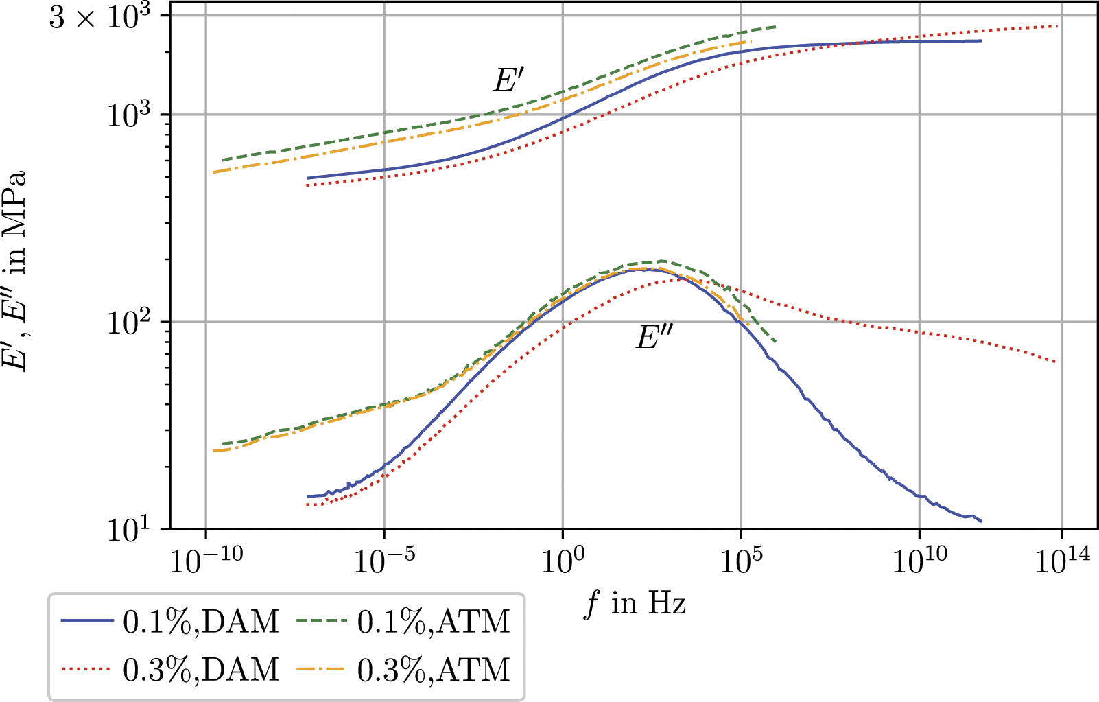

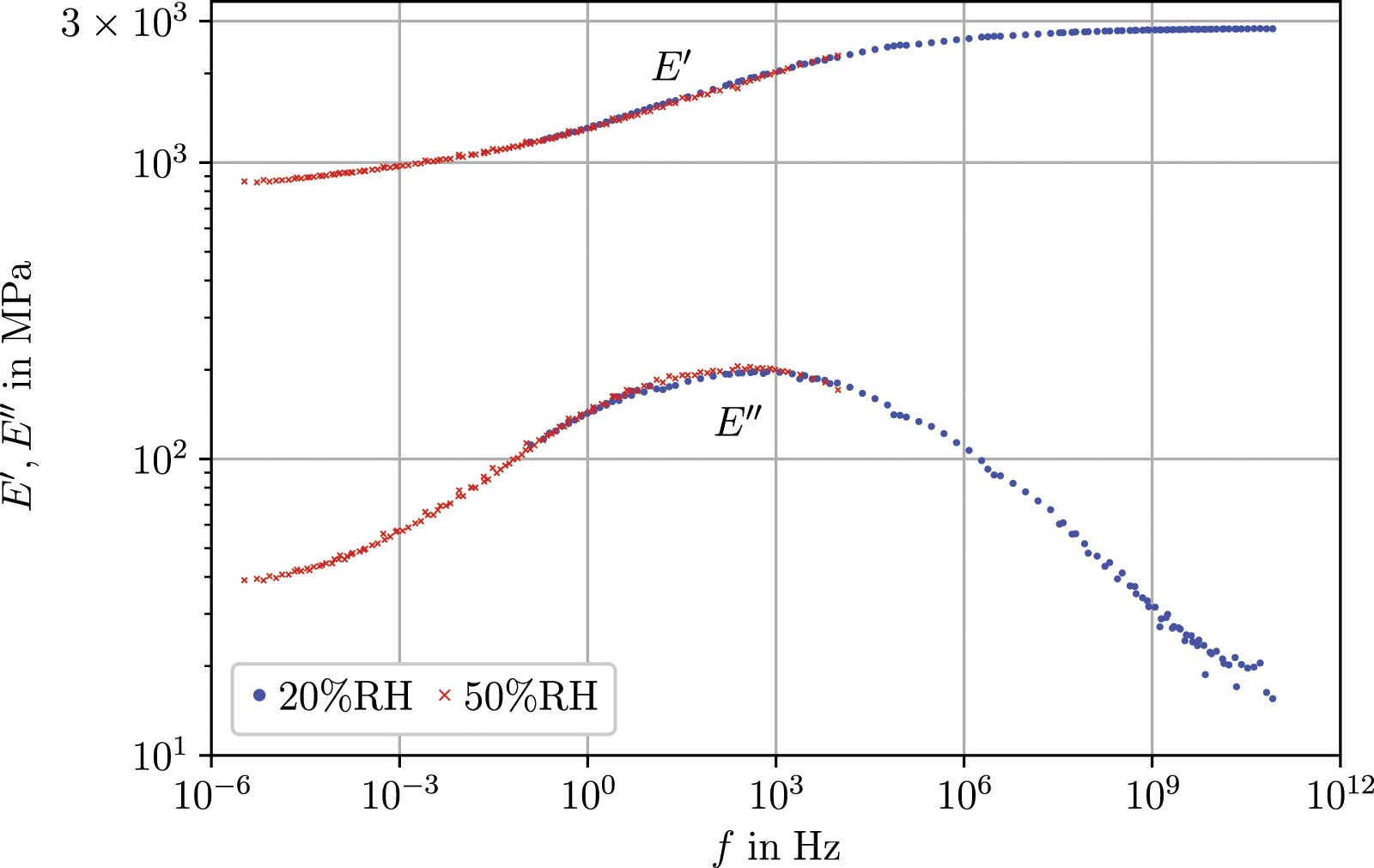
Figure 8 depicts the master curves of the tests performed without humidity control. In terms of a linear viscoelastic behavior, the curves should be identical for different load levels. As the red and the blue curves are not identical, the dried samples show nonlinear behavior at a mean strain ɛ₀ = 0.3%. A load shift cannot be applied as the curve shapes differ. On the red curve, the saddle point of the storage modulus and the maximum of the loss modulus is reached for a higher frequency. Furthermore, the loss modulus is not symmetric as it decreases less strongly after its maximum is reached. Additionally, the shift factors for the higher load are larger resulting in a broader frequency range. For the conditioned samples, nonlinear behavior cannot be detected as the master curves are in good agreement.

The master curves shown in Figure 9 provide a common master curve. In this case, the humidity influence can be modeled by a humidity-dependent glass transition temperature. If instead the same reference temperature is chosen for both master curves, a humidity shift can be seen. The master curves for the tests without humidity control in Figure 8 indicate more complex nonlinear behavior. Only the loss modulus shows a common master curve between 10⁻¹ Hz and 10⁶ Hz. Therefore, the influence of moisture content cannot be modeled by a simple shift in this case.

In Figure 10, the master curves for tests of ATM23/50 conditioned samples with and without humidity control are compared. The curves are in good agreement. In this case, the influence of a missing climate control is not as pronounced. Consequently, changes in mechanical properties due to diffusion do not happen at the measurement temperatures (10 − 70°C) within the time scale of the experiment. This is in agreement with Figure 2 where, for instance, at 80°C no differences were observable for the first 400s of the relaxation test. Note, the sample is subjected to the target temperature for about 4000 s in total if the soak time before the starting of the relaxation test is taken into account.

Figure 10.

Comparison of master curves from tests performed with humidity control (HC) at 50%RH and without humidity control. ATM-23/50 conditioned samples were used, θ_ref = 25°C. (a) Storage modulus. (b) Loss modulus.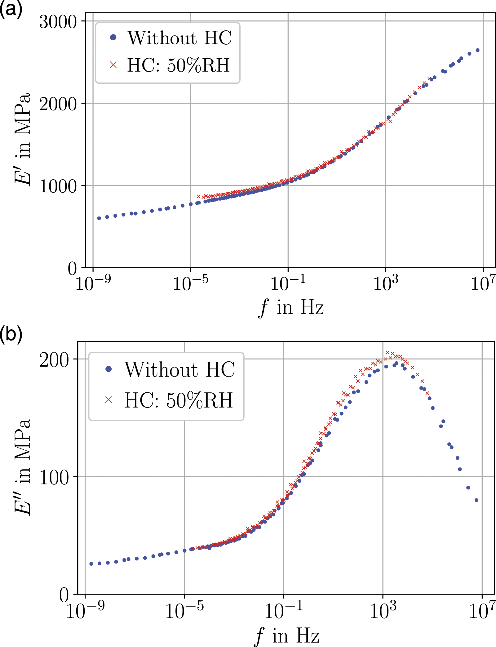

In general, the curves agree well with the asymptotic properties given by equation (5). With increasing moisture content, not all of these properties are evident. The reason is that the corresponding master curves are cut off at some point as the considered temperature range is limited. In all curves, the loss modulus has a pronounced maximum at medium frequencies.

Parameter identification

The discussed master curves can be used as input for a parameter identification. The parameter identification is exemplarily discussed for the tests with DAM samples since these tests cover all properties from equation (5). The relaxation times are prescribed in a logarithmic distribution. First, the load case with ɛ₀ = 0.1% is considered. The largest relaxation time is set to the inverse of the minimum frequency decade, τ_N = 10⁷ s. Vice versa, the smallest relaxation time, τ₁, is set to 10⁻¹² s. For the stiffnesses, lower and upper bounds are defined: The lower bound is set to zero as negative stiffnesses are unphysical. The upper bound is set to 2500 MPa which is nearly the maximum storage modulus. The start values for the optimization are also set to zero. The influence of the number of Maxwell elements and of the weighting factors is investigated. In Figure 11, results are shown for various parameters. The black points depict the master curves. The curves in blue and red show the behavior predicted by the parameter fit. Additionally, the R²-values from equation (33) are given. By increasing the number of Maxwell elements, the fit becomes more precise and smooth, see Figure 11(a), 11(c) and 11(e). Each Maxwell element causes a saddle point in the storage modulus and a local maximum in the loss modulus. The respective positions are defined by the inverse of the corresponding relaxation time. If the number of relaxation times increases, these local saddle points and maxima are blurred. By using 20 elements, a good fit is already obtained. Thus, the rule of thumb that at least one Maxwell element per frequency decade should be used is confirmed.^87,91 If 30 Maxwell elements are used, only the global saddle point and the global maximum can be seen. For large frequencies, the storage modulus is slightly overestimated. The maximum of the loss modulus is slightly underestimated.

Figure 11.

Parameter fit for DAM sample at ɛ₀ = 0.1%, θ_ref = 75°C. Various weighting factors and number of Maxwell elements are considered. The R²-value is given to quantify the quality of the fits. (a) 10 Maxwell elements, a′ = 50%, (b) 30 Maxwell elements, a′ = 100%, (c) 20 Maxwell elements, a′ = 50%, (d) 30 Maxwell elements, a′ = 0%, (e) 30 Maxwell elements, a′ = 50%.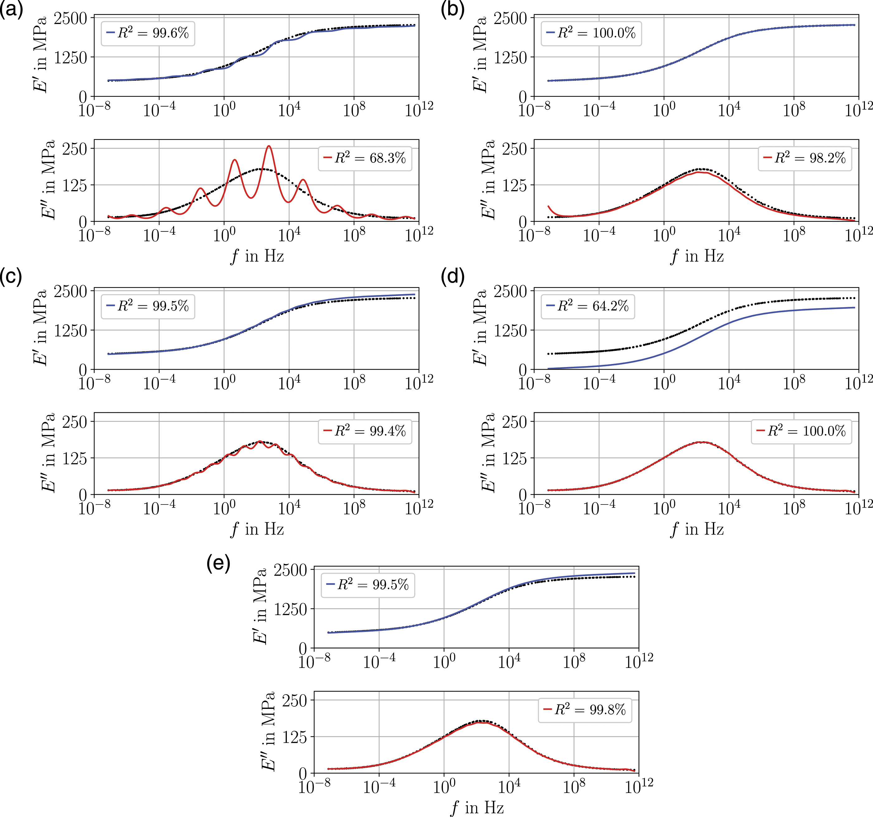

In Figure 11(b), only the storage modulus is considered for the parameter identification, a′′ = 0. Consequently, E′ is perfectly fitted. However, E′′ is poorly fitted for low frequencies and slightly underestimated in the frequency range of 10⁻¹ to 10¹² Hz. In contrast, the results for choosing only the loss modulus as input of the parameter identification, a′ = 0, are depicted in Figure 11(d). In this case, the loss modulus is perfectly fitted. For the storage modulus, an offset can be seen. The reason is indicated by the formula for the loss modulus in Table 4. The loss modulus does not depend on the stiffness of the single spring element E₀. Thus, the start value of E₀ does not change during the optimization. The offset can be minimized by choosing an appropriate start value. To conclude, both storage and loss modulus should be used as input parameters for the parameter identification. Using a′ = a′′ = 0.5 is a reasonable approach.

Figure 12 shows the corresponding stiffnesses and relaxation times for the parameter fits of Figure 11(a), 11(c) and 11(e). The solid lines visualize the respective values of E₀. As E₀ is the lower bound of the storage modulus, the value of E₀ does not change significantly by increasing the number of Maxwell elements. The stiffnesses of the Maxwell elements decrease by increasing the number of Maxwell elements. The maximum of these stiffnesses coincides with the saddle point of E′ and the maximum of E′′ at medium relaxation times.

Figure 12.

Plot of Maxwell parameters from Figure 11 for a′ = a′′ = 0.5 and various numbers of Maxwell elements: N = 10 (blue), N = 20 (red), N = 30 (green). The solid lines show the value of E₀. The dots show the relaxation times and the corresponding stiffnesses of the Maxwell elements.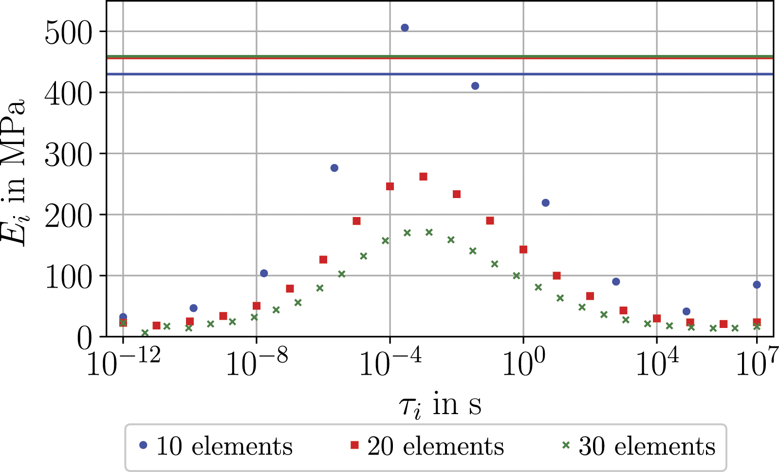

In Figure 13, a parameter fit for ɛ₀ = 0.3% is shown. Compared to Figure 11(e), the storage modulus is more overestimated at high frequencies. The reason may be the asymmetric behavior of the loss modulus. To capture this, the stiffnesses at the corresponding relaxation times are larger. This leads to an overestimation of the storage modulus. Espacially for larger frequencies, the GMM cannot capture this behavior accurately. The corresponding values of the stiffnesses and relaxation times for Figures 11(e) and 13 are given in Table 8 and Table 9.

Figure 13.

Parameter fit for DAM sample at ɛ₀ = 0.3%, θ_ref = 75°C. 30 Maxwell elements are used and the residuals are weighted equally: a′ = a′′ = 0.5.

Summary and conclusion

Polyamide 6 is widely applied as polymeric matrix for fiber reinforced polymers to contribute to a resource-efficient semi-structural material. Despite the outstanding properties of low weight and high specific stiffness accompanied by design freedom for structural parts, PA 6 exhibits also some challenges when environmental influences are taken into consideration. Based on the internal, equilibrium moisture content within the sample, for instance, the characteristic material properties, such as the glass transition temperature, are shifted. In order to take these and other effects into account, the material model needs to be adapted accordingly. Within this work, the thermoviscoelastic material properties for two different humidity levels of PA 6 are experimentally investigated using DMA. By means of the generalized Maxwell model, the hydrothermal effects on the linear viscoelastic material behavior are analyzed. To this end, the following concluding remarks can be made.

Experimental investigations

Relaxation tests

In this context, the tests were performed with and without humidity control inside the testing chamber for a duration of 6 h. For the humidity-controlled tests, the ambient and the internal equilibrium moisture of the sample were the same. In case of no humidity control, after an initial decrease of the relaxation modulus, an increase was observed after 500 s. As per conditioning, the samples exhibited an initial relative humidity of 50%RH, whereas the relative humidity in the testing device chamber was at 35%RH due to environmental conditions. This difference in relative humidity caused a drying of the sample during the measurement inducing changes in the mechanical properties due to the hydrophilic nature of PA 6. A direct comparison between the experiment conducted at controlled and non-controlled humidity, further illustrated this effect. While in the humidity-controlled test no drying of the sample takes place, a typical decreasing course over time results for the relaxation modulus. Consequently, for relaxation tests at times within the range of hours, use of a humidity-controlled testing chamber is recommended.

Temperature-frequency tests

To determine the viscoelastic behavior of the PA 6 material used within this work and to obtain input data for a viscoelastic material model based on generalized Maxwell elements, DMA tests with varying temperature and frequency load were conducted. The evaluation of these tests revealed that the glass transition temperature is shifted by about 10 K for a considered frequency range of three decades. However, a higher influence on the glass transition temperature by humidity load was observed. A comparison between DAM and ATM-23/50 conditioned samples revealed a shift of 50 K for the glass transition temperature.

Humidity sweeps

DMA tests with varying ambient humidity level ranging from 5%RH to 95%RH were performed. The tests were repeated at four different temperatures. The temperature load showed a more significant influence on the storage modulus E′ than the humidity load, however, it should be noted that the samples did not reached equilibrium moisture content during the measurements.

Viscoelastic modeling and parameter identification

Shift method

Based on the method by Bae et al., ⁷⁶ the method of normalized arc length minimization was developed. To account for an increasing x-range by the shifting procedure, the existing method was extended by using the normalized arc length. The method calculates shift factors by global optimization and was applied to temperature-frequency tests. First, horizontal shift factors were determined based on the loss factor. Then, vertical shift factors were calculated based on the storage modulus.

Master curves

Master curves were constructed for various loading conditions and then compared. The following limitations of TTS could be observed:

• TTS failed for DAM sample at a mean strain of 0.5% and an amplitude of 0.25%

• The temperature range for DAM samples was between 20°C and 130°C

• This temperature range is shifted by approximately −30 K for conditioned samples

• Frequencies higher than 20 Hz were not considered

For DAM samples, a load-dependency of the master curves was observed. For the conditioned samples, no pronounced load dependence was detected. By comparing the test performed under humidity control at 50%RH and the test with a conditioned sample, no differences were evident. In contrast to the findings based on the relaxation tests with and without humidity control, a humidity-controlled testing chamber is not necessarily required for temperature-frequency tests. The testing time is within time scales where diffusive processes are not that pronounced as to cause significant differences between test data.

Parameter identification

The master curves of the DAM samples were exemplarily used as input for a GMM parameter identification. The weighted residuals of storage modulus and the loss modulus were considered for least squares optimization. It was shown that both, storage and loss modulus, should be accounted for. Furthermore, it was confirmed that between one and two Maxwell elements per frequency decade are needed for a good fit. For a mean strain of 0.1%, a good fit is observed. At a mean strain of 0.3%, the fit revealed inaccuracies. This implicates a transition to the nonlinear viscoelastic regime which is the scope of future work.