The present article is concerned with modeling the viscoelastic behavior of Polydimethylsiloxane (PDMS) in large-strain regime. Starting from the basic principles of thermodynamics, an incremental variational formulation is derived. Within this model, the free energy density and dissipation function determine elastic and viscous properties of the solid. The main contribution of this paper is the estimation of the parameters in the proposed phenomenological model from measurements conducted on Sylgard184 samples. This non-linear material model simplifies to a Prony-series representation in frequency domain in case of small deformations. The coefficients of this Prony-series are detected from dynamical temperature mechanical analysis measurements. Time-temperature superposition allows to combine measurements at different temperatures, such that a sufficiently large frequency range is available for subsequent fitting of Prony-parameters. A set of material parameters is thus provided. The incremental variational formulation directly lends itself to finite element discretization, where an efficient and stable choice of elements is proposed for radially symmetric problems. This formulation allows to verify the proposed model against experimental data gained in ball-drop experiments.
Silicone-based polymers, like Polydimethylsiloxane (PDMS), are known for their high flexibility and excellent damping properties. Thermal and chemical stability, corrosion resistance, and optical transparency add to the features of these materials. Not least their easy accessiblity at low cost and simple generation of samples allow for numerous applications in science and engineering. We cite the recent review papers by Ariati et al. (2021) and Zaman et al. (2019), both of which provide a great overview over the properties and applications of PDMS.
Typical applications of PDMS include, for example, microfluidics, where channels are required for filtering, separating and mixing fluids (cf. Borók et al., 2021), the insulation of electronic components, or coating of sensitive materials to protect them from external effects (cf. Eduok et al., 2017). In these applications, the damping nature of PDMS is of high advantage. An increase of the damping behavior could be realized through micro-structure design of sponges in Zhu et al. (2017). Treatment of surface layers was used to generate custom wrinkling patterns in specimen in Knapp et al. (2021).
The reliable realization of many of these applications requires accurate and efficient simulation techniques to predict the behavior of the system under consideration. Due to the high flexibility of PDMS, such a model must be fit to represent large deformations, and the damping properties have to be characterized properly.
Although frequently used in biomechanical or medical applications, the mechanical characterization of PDMS is not yet sufficiently accurate. Concerning the hyperelastic behavior, Nunes (2011) proposed a simple shear strain test to obtain material parameters for Mooney-Rivlin type materials. They proposed to use a variant to the classical Mooney-Rivlin material law to better fit their measurements. Later, Cardoso et al. (2018) fitted different hyperelastic material laws, including Mooney-Rivlin, Ogden, and Yeoh models. The influence of surface patterns on the elastic response was analyzed by Lee et al. (2021). Characterizations of the damping properties are scarce, Lin et al. (2009) experimentally detected Prony-parameters from punch tests and a specially developed dynamical mechanical analysis (DMA); however, the frequency range of this DMA is limited and the influence of temperature is not treated. Deguchi et al. (2015) measured storage and loss modulus at a single frequency of 1 Hz for a range of temperatures and several PDMS polymers. In their technical note, Long and Brown (2017) treat the applicability of time-temperature-superposition to Sylgard 184.
We propose an approach for modeling and subsequent simulation of viscoelastic solids, which we apply to Sylgard 1841 in particular. Our approach ensures thermodynamic consistency in large deformation regime, as the incremental formulation is based on the Clausius-Duhem inequality and is defined not only through hyperelastic energy densities, but also through a dissipation function to model viscoelastic losses. In Kunzemann et al. (2023), a similar characterization was extended to include electromechanical coupling due to dielectric effects. To determine the material parameters used in these functions, a specimen of Sylgard 184 is subjected to dynamical temperature mechanical analysis (DTMA) in a limited range of frequencies. Through time-temperature superposition, a sufficiently large range of frequencies can be covered. From this data, a set of material parameters for a Prony-series expansion is found through a non-negative, non-linear least squares fit, similar to Kraus et al. (2017). These Prony-parameter directly correspond to the parameters of the proposed non-linear model.
In order to verify the proposed constitutive model, a finite element model of a ball-drop experiment is set up. The ball size and drop height are chosen in such a manner that large deformations will occur. The incremental variational formulation can directly be transferred to the context of finite element simulation. A classical stable pair of displacement-pressure elements is proposed to account for the incompressible nature of PDMS. Additional degrees of freedom for viscous strains satisfy the incompressibility condition exactly for radially symmetric problems. Time integration using the Newmark- scheme in variational context avoids any numerical damping.
The remainder of this paper is organized as follows: After the introduction, the constitutive model based on a hyperelastic potential, viscous contributions, and a dissipation function is discussed. Next, the correspondence of this non-linear model to a Prony-series expansion is discussed. The estimation of Prony-parameters from DTMA measurements is conducted using time-temperature superposition as well as non-negative least squares approximation. An incremental variational formulation, which replaces D’Alembert’s principle in dissipative processes, is derived and shown to be equivalent to classical viscoelastic models. This directly leads to the definition of a finite element model for radially symmetric problems in the following section. Finally, computational and experimental results are compared for a ball-drop experiment.
2. Viscoelastic modeling
2.1. Kinematics
We consider a body consisting of a viscoelastic material. Each material point is identified by its position vector in reference configuration. The motion of the body is described by a time-dependent mapping , which maps each material point to its current spatial position at time , . We use standard notations for all relevant kinematic quantities, starting with the displacement field . Throughout the following, we identify derivatives of fields with respect to reference coordinates by using capital operators. Derivatives with respect to spatial coordinates are identified using lower case operators.
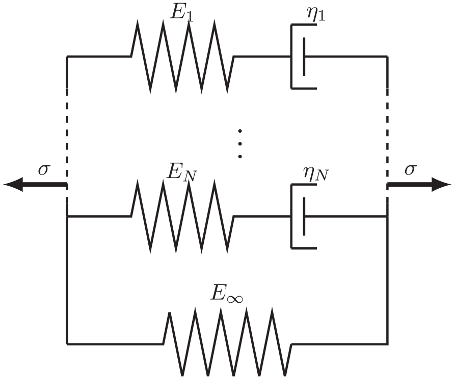
The deformation gradient is then defined as . For modeling large deformation viscoelasticity, an extension of the one-dimensional rheological standard solid model Haupt (2013) is proposed. In the standard solid model, also known as Wiechert model, a single spring element and spring-dashpot combinations in series, also known as Maxwell element, are connected in parallel, see also Figure 1.
Linear, one-dimensional rheological Wiechert model for viscoelastic solids.
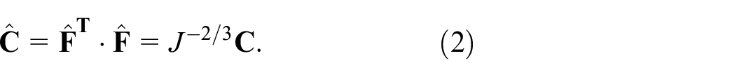
For the representation of incompressible elastomers, a splitting of the deformation gradient into its volumetric and isochoric components is adopted, with a hat denoting the isochoric part with . Based on the above definitions, the right Cauchy-Green tensor and isochoric component of the right Cauchy-Green tensor are given by,
For incompressible materials, its valid to say that we have which leads to and therefore leads to .
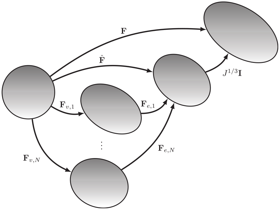
At large deformations, as an extension of the linear model, independent stress-free, volume-preserving intermediate configurations are postulated, to which the respective elastic material laws can be applied. For each of these configurations, the isochoric part of the deformation gradient decomposes multiplicatively into an elastic part and a viscoelastic part , see Figure 2, or see for example, Ask et al. (2012),
Representation of the multiplicative decomposition.
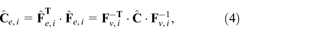
Above, the viscoelastic parts of the deformation resemble the transformation to the stress-free intermediate configuration. The tensor is not necessarily compatible, which means there is no continuous displacement field generating a global intermediate configuration; the decomposition is purely local. However, it is assumed that the viscoelastic contributions are modeled in an isochoric way, such that for all . Based on the elastic isochoric part of the deformation gradient , the corresponding elastic and viscoelastic Cauchy-Green tensors can be defined via,
2.2. Constitutive equations
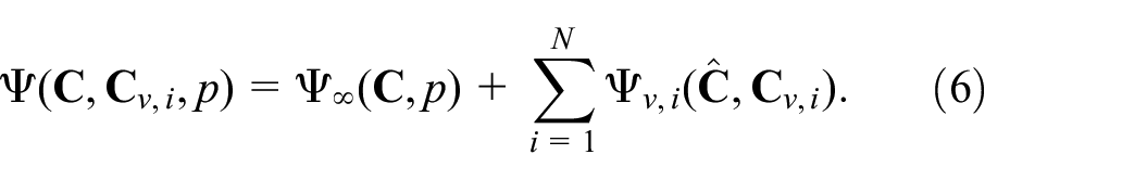
In the following, a thermodynamically consistent model for a viscoelastic material shall be developed. To this end, the free energy density shall be defined for independent Cauchy-Green tensor or deformation gradient . The viscoelastic Cauchy-Green tensors will serve as internal variables, and pressure will act as a Lagrangian multiplier for the incompressibility constraint.
The free energy is assumed to be additively composed of several independent potentials, compare Ask et al. (2012). We consider a decomposition into a hyperelastic potential and a viscoelastic energy densities , which shall be defined in the following,
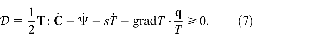
For the formulation of the constitutive equations we use the framework of the Clausius-Duhem inequality. This inequality states essentially that the dissipation is non-negative (cf. Doghri, 2013), which can be written as,
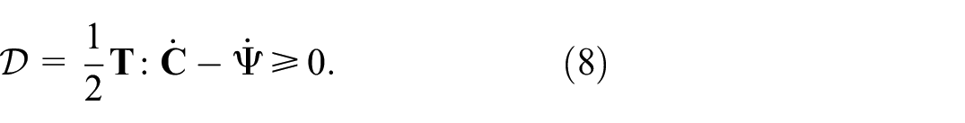
Above, is the second Piola-Kirchhoff stress, is the absolute temperature, is the entropy, and is the heat flux vector. Since we assume isothermal processes in the following, with and no external heat flux , the expression simplifies to,
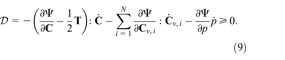
Computing the rate explicitly, equation (8) becomes,
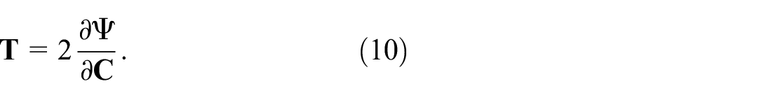
Equation (9) implies the classical constitutive equations for the second Piola-Kirchhoff stress as,
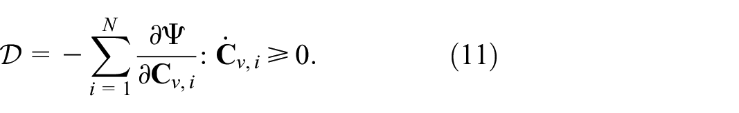
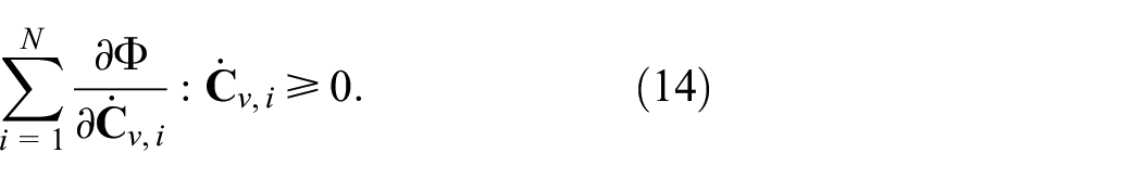
Moreover, pressure acting as a Lagrangian multiplier ensures the condition of incompressibility as . The reduced dissipation inequality states that the negative inner product of generalized driving forces and viscous strain rates is non-negative,
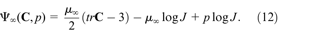
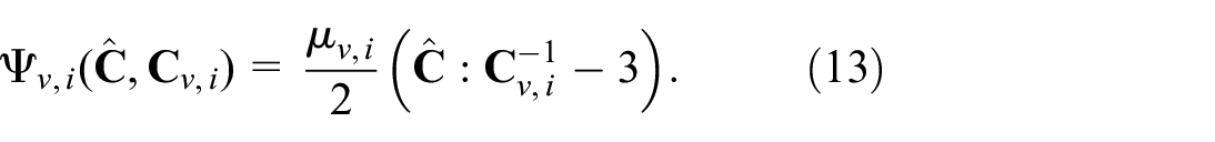
Let us collect specific representations for the energy densities constituting the augmented free energy . The elastic part of the free energy will be governed by an incompressible Neo-Hookean hyperelastic potential. We use for the long-term shear modulus,
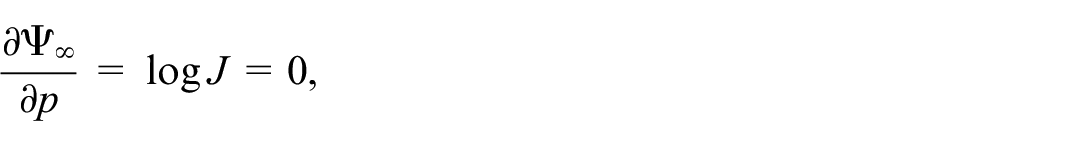
For small strains, the Neo-Hookean material model reduces to a linear correlation, accurately described by Hooke’s law. Pressure serves as a Lagrangian multiplier to ensure the incompressibility constraint,
such that .
Concerning the multiplicative decomposition, a similar incompressible Neo-Hookean hyperelastic potential models the elastic energy for with shear modulus . As , we use the representation,
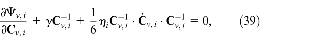
Viscoelastic evolution is defined implicitly through a dissipation function which satisfies,
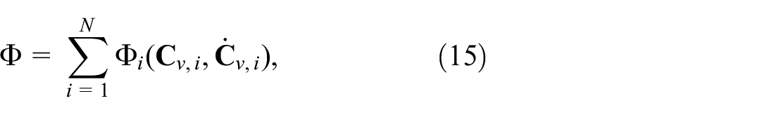
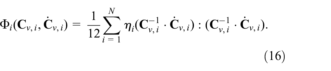
As for the free energy densities, we also assume the dissipation function to be composed additively from contributions due to the internal variables . Each of the terms is governed by a viscosity parameter . To be specific, we use,
with,
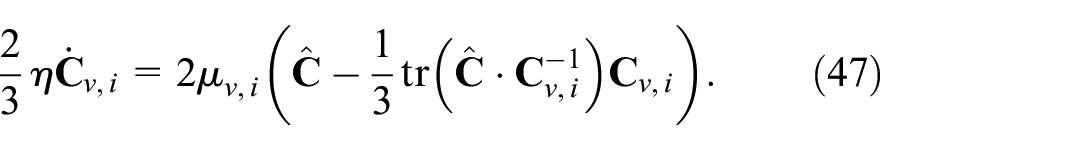
With the choice of equations (16), (14) is satisfied. We justify this choice in the third section Incremental minimization principle by deriving a variational formulation and deducing the according flow-rule, equation (47). To analyze the implications of free energy and dissipation function on the evolution of , an incremental variational formulation based on these quantities is posed later. There, we see that classical viscoelastic material models are reproduced for the above choices. Additionally, the incremental variational formulation can directly be transferred to a finite element discretization, which we do for the special case of rotationally symmetric problems.
3. Temperature-time shifting and parameter fitting of measured data
3.1. Linear viscoelasticity
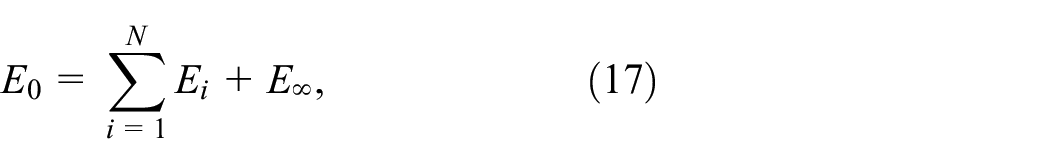
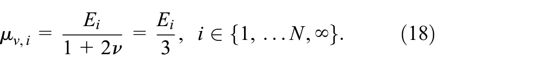
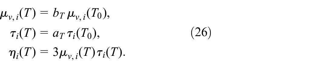
The viscoelastic parameters such as the long-term modulus and the viscous properties and of our non-linear constitutive model are characterized from small-strain measurements, such that an identification using the linear Wiechert model is valid. Within this model, each spring is characterized through its elastic modulus . The long-term modulus of the system equals , that is, the modulus of the single spring. Its instantaneous modulus can be found as,
for a thorough discussion we refer to Haupt (2013). For incompressible materials with a Poisson ratio of , shear moduli and Young’s moduli are connected via,
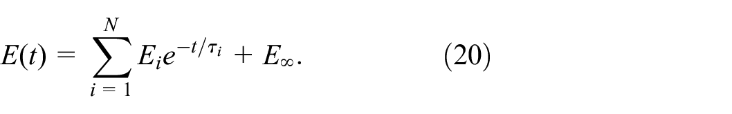
Additionally, defines the relaxation time of the Maxwell element by,
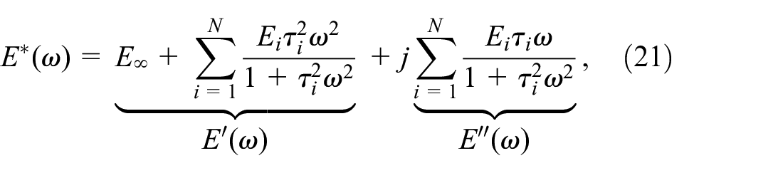
Representation (20) is often referred to as Prony-series. After Fourier transformation to frequency domain, one obtains the more common series expansion,
where is termed the complex modulus of the material. In this context, the real part is called storage modulus and the imaginary part is known as the loss modulus , see Tschoegl (2012).
Furthermore we define with the instantaneous modulus as defined in (17). Following our model, the material is now fully characterized when estimating the parameters and as well as the long-term modulus . We often refer to as the order of the Prony-series.
3.2. Dynamical temperature mechanical analysis
To determine these Prony-parameters from experiments, dynamical temperature mechanical analysis (DTMA) measurements have been performed. These DTMA measurements provide storage and loss modulus over a given frequency range at different temperatures. The measurements were carried out on a Netzsch DMA GABO Eplexor®500N HT.
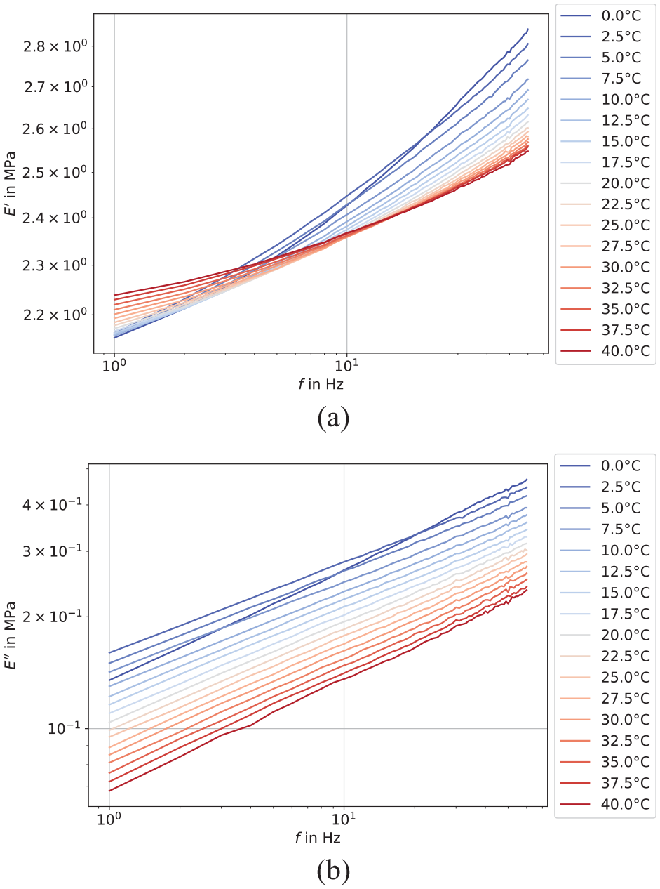
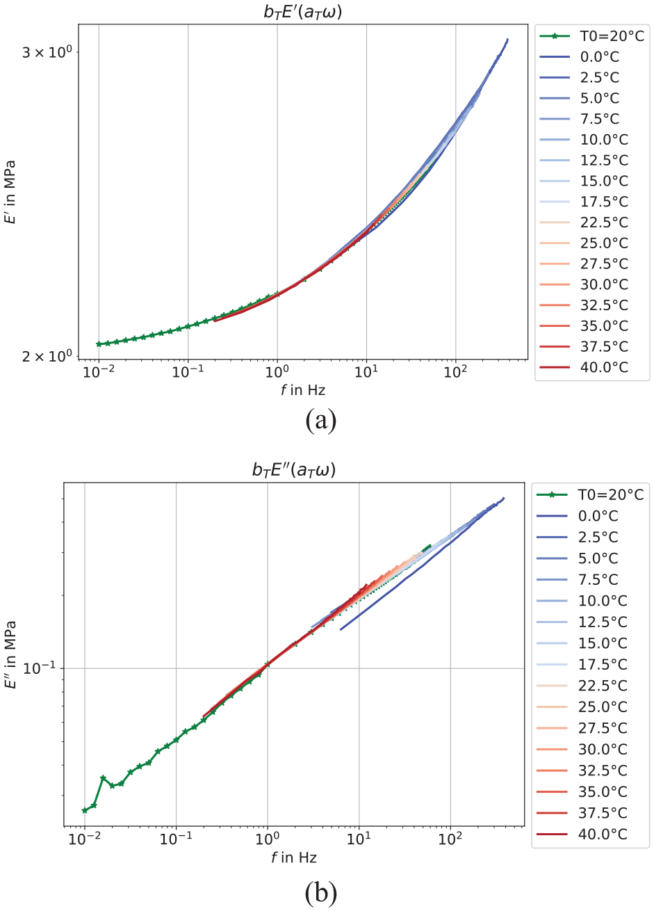
The specimen material, Sylgard 184, was prepared using a (base:crosslinker) mixing ratio by weight. The mixture was stirred for 5 min and then cast into a mold and cured at for 24 h. To create the DTMA samples, a square mold was used, and then cut to size. The cylindrical samples used for the ball-drop tests were produced using a corresponding circular mold. The production of samples is described in detail in Preuer (2018). The dimensions of the sample were and a clamping length of 20 mm was chosen. The static strain was 3%, the dynamic strain 2% with a control range of 0.0045% and the pre-stress was 0.05 MPa. The pre-cooling time in the temperature chamber was at least 2 min. Measurements were taken in the range to in steps between 0 and 100 Hz. Each measurement contains 12 cycles, from which 10 are used to compute the average. Due to resonance peaks for all curves at around 72 Hz we did not use the entire measurement curve, but only from 0 Hz to 60 Hz, as shown in Figure 3(a) and (b).
This range is too small to describe the whole range of frequencies excited in applications. The time-temperature superposition principle (TTSP) allows to generate a so-called master curve that can cover a much larger frequency spectrum from measurements at different temperatures. Conversely, predictions can also be made about the long-term behavior, see also Brinson and Brinson (2015), Ferry (1980).
3.3. Time-temperature superposition
Concerning time-temperature superposition, Sylgard 184 is treated as a thermorheologically complex material, cf. Klompen and Govaert (1999). In the modeled area, the cross-linked material is well above the glass transition temperature and the melting temperature , cf. Dewimille et al. (2005). This results in a melt-like mobility, which can be described by means of thermorheologically complex modeling. The selected approach combines the classic TTSP for solid polymers (complex Young’s modulus) and the TTSP for polymer melts (complex viscosity). Thus, horizontal frequency shifts as well as vertical shifts in the modulus are applied. In Tschoegl et al. (2002), the following general form of time-temperature shifts was identified as,
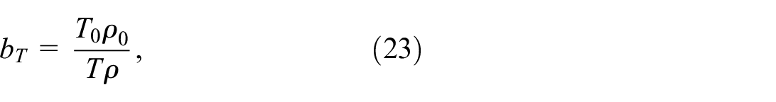
Shifting parameters and allow to transfer the material’s modulus from reference temperature to any other temperature , at least within a certain temperature range. A simple approach for shifting the modulus is given by,
where and are the mass density of the polymer at and . Since we assume no relevant density differences within the sampled temperature range of –, this density ratio is neglected in the following.
For the horizontal frequency shift a large variety of models can be found. Probably the one most commonly used is the Williams-Landel-Ferry model (WLF). However, a main criterion for this is free-volume availability, which is despite the amorphous morphology at ambient temperature limited by the intermolecular bonds created in cross linking. As shown in Lomellini (1992), the WLF model can be used very well for a temperature range of .
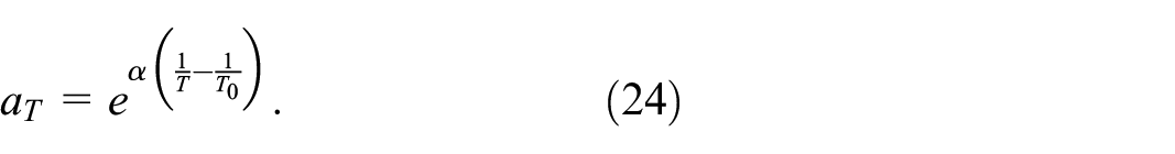
Clarson et al. (1985) and also Li et al. (2006) found that the glass transition temperature of Sylgard 184 is in the range of and the melting temperature lies between and . This implies that the WLF model is not applicable to Sylgard 184 at ambient temperatures. Lomellini (1992) states that in this relatively high temperature range of °C the so-called Arrhenius equation is applicable,
The parameter is independent of temperature, but can be computed from the activation energy and the universal gas constant . We use the DTMA measurement data to compute , and thereby the activation energy , using a least-squares method.
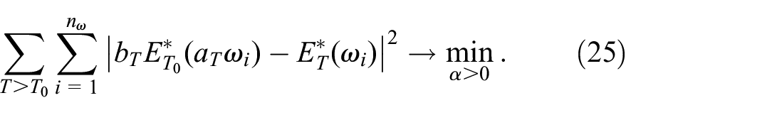
In order to estimate , at reference temperature of measurements within an extended frequency range were conducted. While it is of course not possible to extend this range towards higher frequencies, measurements for lower frequencies approaching zero could easily be conducted; the results are displayed in Figure 4. Then, data sets for temperatures from to were used to determine the unknown shift parameter , as higher temperatures correspond to lower frequencies. A least squares method is used to find the optimal parameter in order to minimize the squared vertical distance of the respective data curves when shifted by and as in (23) and (24), respectively. As the shifted frequencies for the data points do not coincide in general, a linear interpolation of the reference data in between data points is used instead. For the frequencies at which DTMA data is available, the least-squares problem finally reads,
Master curves for storage and loss modulus at gained through time-temperature superposition: (a) storage modulus at , (b) loss modulus at .
For the available DTMA data, this procedure results in . Then, both the storage and loss moduli from all DTMA data temperatures can be shifted according to (22) to get a master curve at temperature as shown in Figure 4. These shifted data sets are used in the subsequent detection of Prony-parameters; the additional data in the extended frequency range for temperature are not included in this process anymore.
3.4. Prony-parameters
Once data in an extended frequency range has been generated using the TTSP, Prony-parameters as well as and can be detected. To this end, a non-linear least-squares optimization problem for the unknown Prony-parameters needs to be solved. For the presented data, the non-negative least squares based routine curve_fit provided within python’s scipy package could be applied successfully.
This function works with complex data sets, and thereby ensures that the parameters determined are accurate for both the storage and loss modulus. Moreover, range conditions have to be met for the different parameters. A minimal set of these conditions is to seek for
a positive long-term modulus ,
positive relaxation times ,
relative viscoelastic moduli ,
satisfying additionally .
Simple range conditions like the former three items can be included in the parameters passed to the least-squares fitting routine. The latter condition has to be verified manually, once the parameters are computed. As one often observes in non-linear problems, choosing a feasible starting value is of utmost importance. We observed that setting all values to one worked well when seeking the long-term modulus equivalent to 1 MPa.
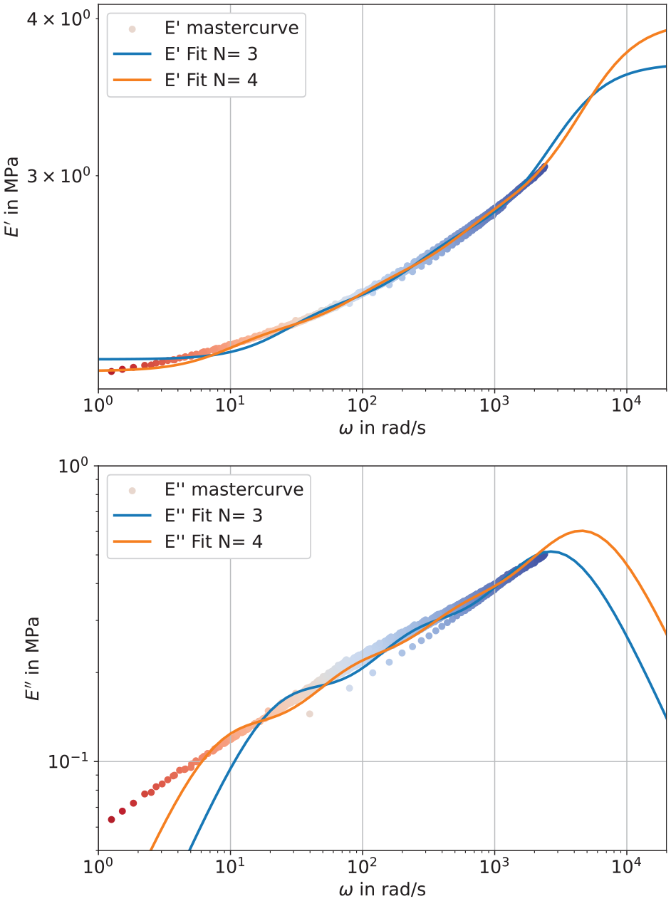
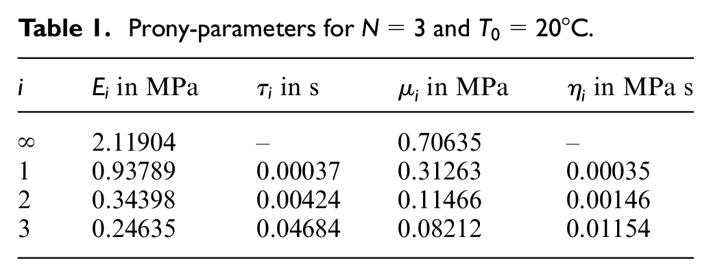
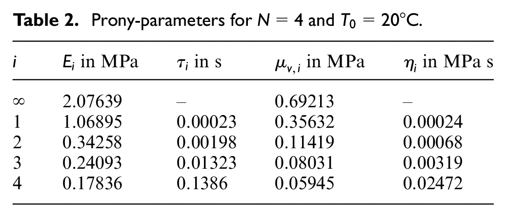
Finally, the order of the Wiechert model has to be chosen in accordance with the available data set. As a rule of thumb, good approximation is obtained when using one Maxwell element per measured frequency decade. Since after TTSP, measurements are available for frequencies from 0.1 Hz up to almost 1000 Hz (see Figure 4), fitting Prony-parameters for models of third and fourth order seems appropriate. The respective results are depicted in Figure 5. Tables 1 and 2 show the corresponding Prony-parameters , and as well as the shear moduli and viscosities computed from these values via (18) and (19).
Fitted Prony-series, comparison and .
Prony-parameters for and .
in MPa
in s
in MPa
in MPa s
2.11904
–
0.70635
–
1
0.93789
0.00037
0.31263
0.00035
2
0.34398
0.00424
0.11466
0.00146
3
0.24635
0.04684
0.08212
0.01154
Prony-parameters for and .
in MPa
in s
in MPa
in MPa s
2.07639
–
0.69213
–
1
1.06895
0.00023
0.35632
0.00024
2
0.34258
0.00198
0.11419
0.00068
3
0.24093
0.01323
0.08031
0.00319
4
0.17836
0.1386
0.05945
0.02472
In both Tables 1 and 2, we note that the relaxation times are distributed more or less evenly across the measured decades, as is to be expected due to Tschoegl (2012).
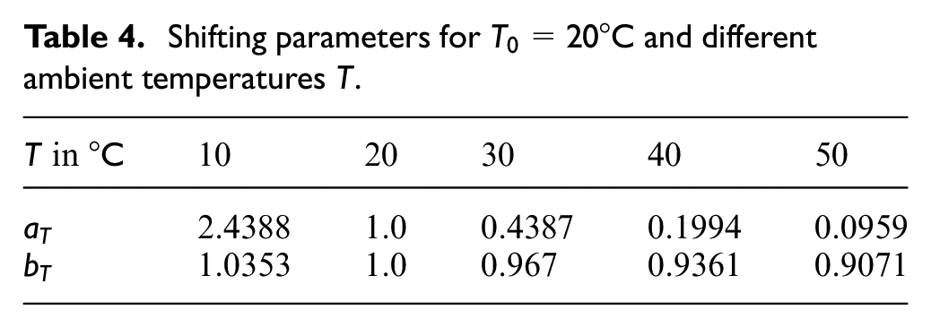
As parameters at reference temperature are determined, according parameters for different ambient temperatures can be computed through the time-temperature superposition principle (22), leading to
Parameters and are defined in (24) and (23), values for specific temperatures are listed in Table 4.
4. Incremental minimization principle
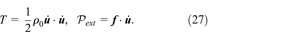
Having determined the relevant constitutive parameters, we now seek a finite element formulation for the problem at hand. As a starting point, a variational formulation for viscoelastic solids is derived from an incremental minimization problem. A similar procedure has been presented for modeling various dissipative processes by the group around Miehe, we cite non-exhaustively Miehe (2002); Miehe et al. (2002, 2011). For reasons of simplicity of presentation, we restrict ourselves to the case of a conservative volume force density . With the mass density, the kinetic energy density and local power of external forces read,
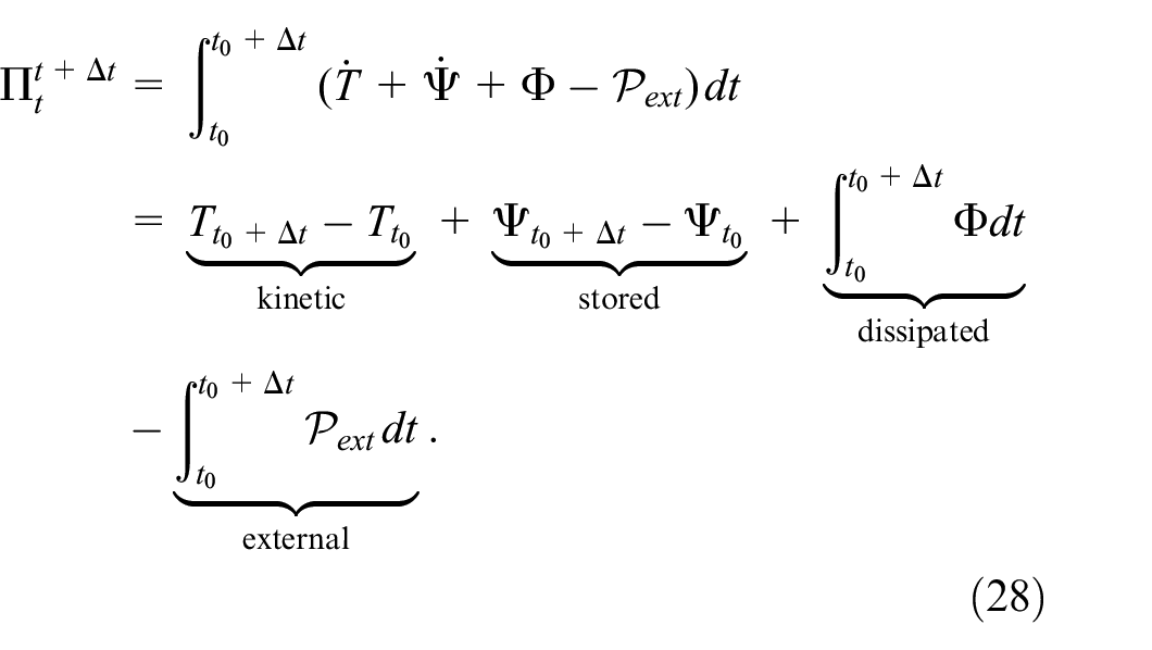
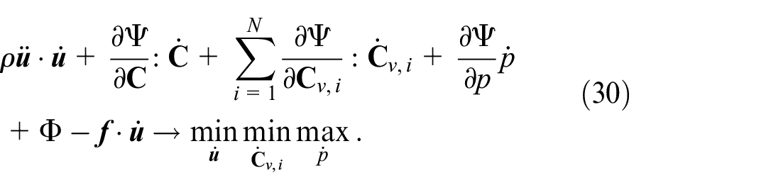
Consider a finite time step with known initial conditions at time . We introduce the incremental potential for this time step as,
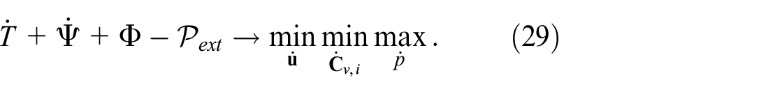
The incremental potential is then minimized with respect to all admissible displacements and viscoelastic internal parameters, and maximized with respect to hydrostatic pressure. For time step size approaching zero, we arrive at,
We can now rewrite equation (29) for the specific choice of free energy and get,
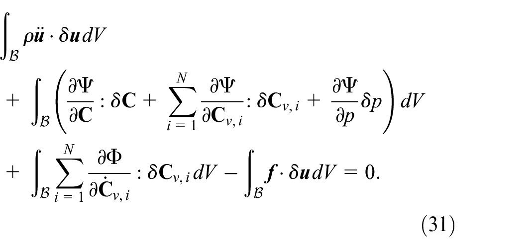
Under common assumptions on convexity and smoothness of the involved energies and dissipation functions, the optimization problem is equivalent to finding critical points as solutions to the corresponding variational equation, also known as D’Alembert’s principle,
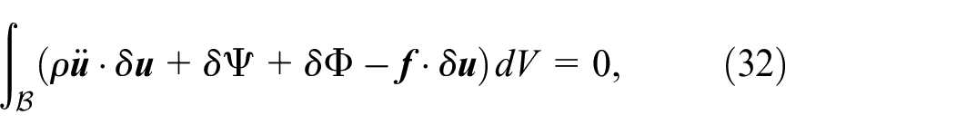
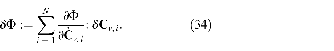
For a simplified presentation, we rewrite D’Alembert’s principle in more compact form, although abusing notation concerning the variation of the dissipation function,
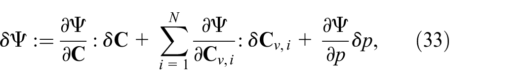
with,
and
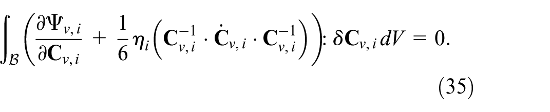
The variational equation (31) implicitly defines the evolution law for for arbitrary but fixed index . We show that, for the proposed choice of dissipation function from equation (16), the standard model as for example, proposed by Haupt (2013) is re-established. We collect all terms containing from equation (31), and obtain,
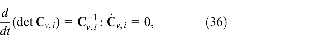
Since , we observe for its rate and variation,
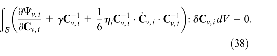
Thus, a contribution of the form can be added without changing the equation (35), which leads to,
Here, is an arbitrary constant that still has to be determined in the following. As is otherwise arbitrary, the equality holds in classical sense,
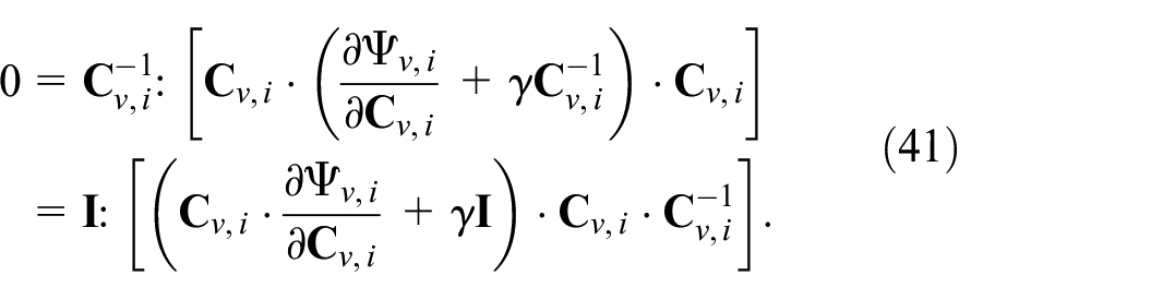
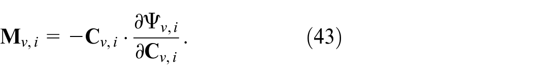
Above, we introduce as the Mandel-type stress tensor,
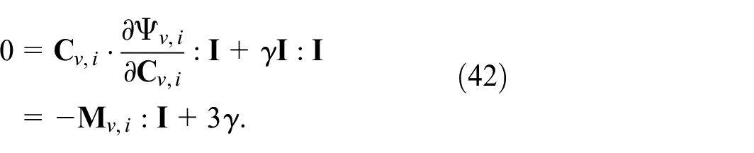
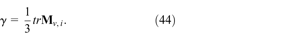
With this, we finally have an expression to determine the unknown parameter ,
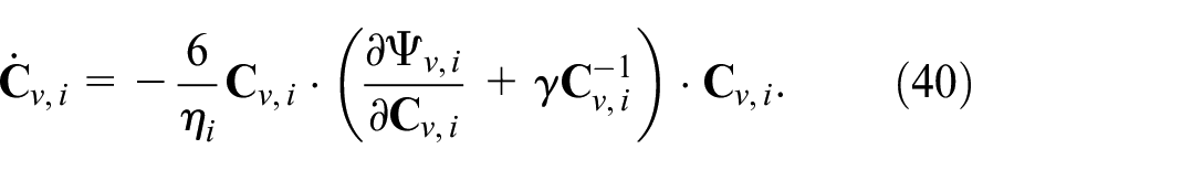
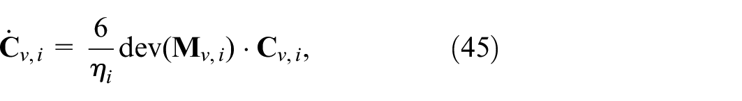
We can now substitute back into equation (40) and after a few algebraic manipulations we get,
which is stated in similar form by Ask et al. (2012) for viscoelastic electrostrictive polymers.
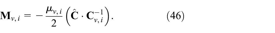
To compare the final evolution law to standard theory, we explicitly compute the Mandel-type stresses for the viscoelastic potential from equation (13) and obtain,
After combining the two equations (45) and (46) we finally obtain the evolution law for as stated in Haupt (2013),
Note that, in the finite element approach proposed below, this evolution equation is not integrated explicitely, but is implied implicitely through the incremental variational formulation including variations .
5. Finite elements for radially symmetric problems
For radially symmetric problems, a finite element model respecting incompressibility of the viscous strains explicitely can be devised as follows. This setup is designed such that it allows for verification against various measurement setups, like the ball-drop experiment in the last section to determine rebound resilience.
5.1. Spatial discretization for radially symmetric problems
Let the body as well as all external forces and kinematic constraints be in accordance with radial symmetry. Without restriction of generality, we consider as axis of rotation. Deformation gradient and right Cauchy-Green are defined in the standard way, assuming that the solution is independent of the angular coordinate .
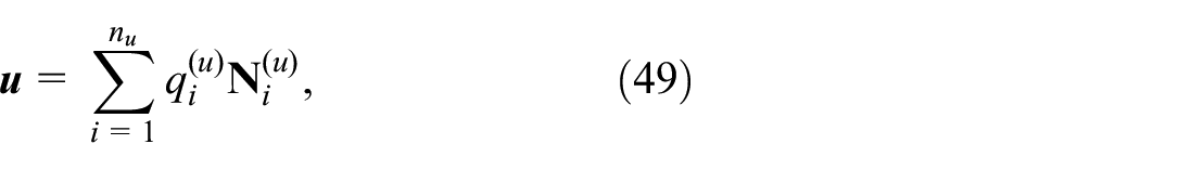
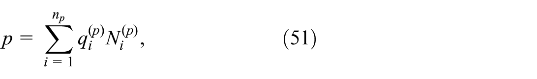
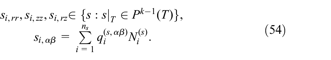
Assume to be a triangular finite element mesh of the section of under consideration. Concerning the elastic problem, we propose to use the pair of displacement-pressure elements as proposed by Taylor and Hood (cf. Taylor and Hood 1973), where both and are represented by continuous basis functions and respectively, and the approximation order for is one higher than for . Additionally, kinematic boundary conditions on the boundary part have to be satisfied. Summing up, finite element approximations for and satisfy,
with meaning the space of bivariate polynomials of order on triangular elements .
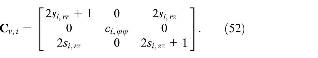
In addition, it is necessary to provide a finite-dimensional approximation for the viscoelastic internal variables . Here, it is important that the kinematic constraint of incompressibility is satisfied by construction. For a rotationally symmetric setting, this can be achieved by a non-linear representation of in terms of the independent viscoelastic strains , and . The viscoelastic Cauchy-Green tensor respects the axisymmetric structure,
Component is chosen such that the incompressibility constraint is satisfied a-priorily, which implies,
The viscoelastic strains and are defined element-wise polynomial, without continuity, one polynomial order lower than the displacements,
5.2. Time integration
Introducing the finite element discretizations equations (50), (51), and (54) in D’Alembert’s principle (31) leads to a system of ordinary differential equations for the degree of freedom vector . As the physical problem includes accelerations and viscoelastic strain rates as well as the Lagrangian multiplier , a differential-algebraic system of equations is generated after spatial discretization. It is well known that the Newmark- scheme is well-suited to solve differential-algebraic equations of index 2, where the choice of parameter further determines its numerical damping properties.
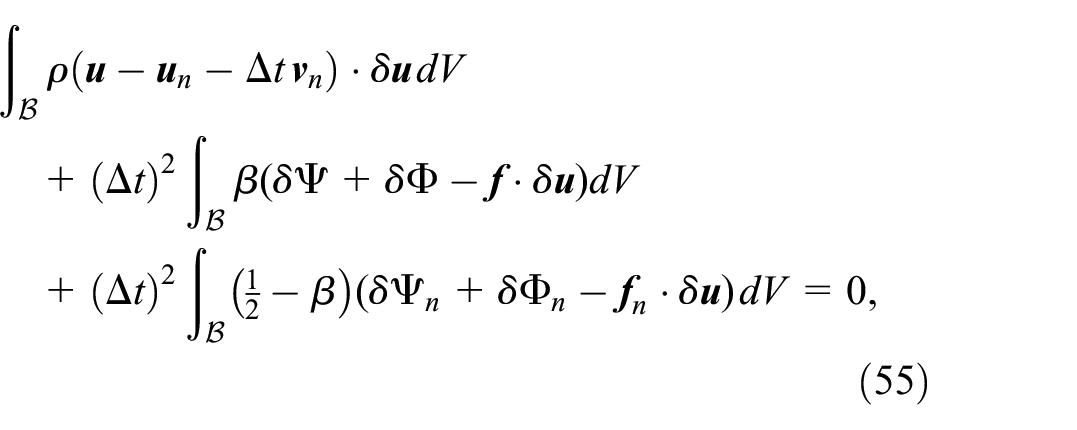
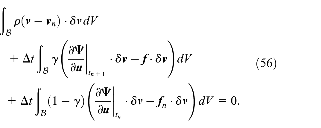
We shortly present the Newmark- scheme adapted for the viscoelastic problem at hand. To this end, we assume that velocities are approximated by an independent linear combination of displacement basis functions , via additional degrees of freedom . For any time step , the quantities as well as , (or rather the viscoelastic strains and strain rates ) at time are assumed to be available from the previous step. According updates and at time are to be computed, where we omit as an index in favor of brevity of presentation. The Newmark- scheme interpreted in terms of the underlying variational equations leads to the coupled non-linear system, where we use as the (independent) variation of the velocity ,
Note that equation (55) does not only implement the Newmark integration scheme for the displacements, but also the incompressibility constraint via and the evolution law for the viscoelastic strains as indicated by the dissipation function. The variation of the dissipation function is to be understood in the same manner as in equation (32).
6. Validation
To validate the material characterization developed above, we present a comparison of computational results to measurements for a ball-drop test setup. Ball-drop tests are frequently used to determine the rebound resilience of materials by comparing the original drop height to the rebound height of the ball. When varying temperature, drop height as well as size and mass of the ball, changes in the rebound resilience are of interest.
For the purpose of computational realization we use the open-source software package Netgen/NGSolve2. Via a python interface, the developed variational time stepping scheme (55)–(56) can be defined symbolically; all proposed finite element spaces are available at arbitrary order. Automatic differentiation takes care of computing correct tangent stiffnesses in a straightforward manner.
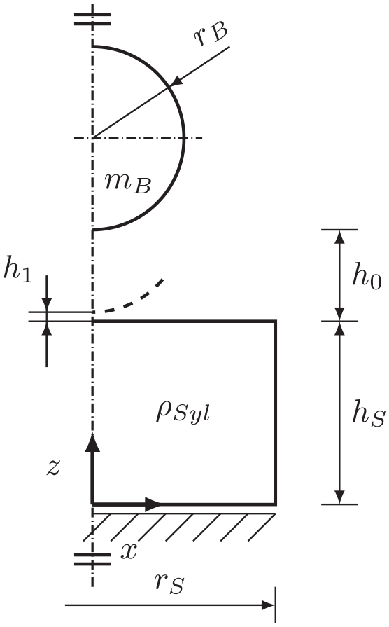
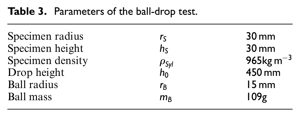
As sketched in Figure 6, we consider a cylindric specimen made from Sylgard 184 with a radius of and a height of . A steel ball of radius and mass is dropped from an initial height of above the cylinder’s surface. With these parameters, large local deformations exceeding 30% can be seen in the later results. All parameters are once again summarized in Table 3.
Computational setup of the ball-drop test.
Parameters of the ball-drop test.
Specimen radius
Specimen height
Specimen density
Drop height
Ball radius
Ball mass
A finite element model exploiting the model’s radial symmetry is generated, where the finite element mesh consists of triangular elements. Third order elements are used in simulations, which results in a total of displacement degrees of freedom. While the proposed material characterization is employed to describe the cylindric specimen, the ball is modeled as linear elastic body with Young’s modulus and Poisson ratio . We choose a penalty-formulation for frictionless contact to describe the interaction of ball and PDMS. In experiments, the polymer’s surface is powdered to reduce friction and adhesion effects to a minimum.
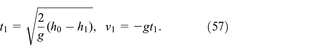
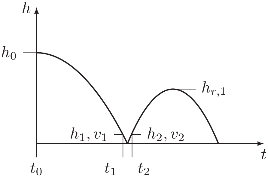
Assume to denote the time at which the ball is released. The actual simulation is restricted to the time interval around the ball’s first impact. To be concise, time stepping is initialized for the ball at height , which is close to the specimen’s surface. This results in an initial time an initial velocity set to,
In Figure 7, these time instants as well as the corresponding velocities and observed heights are visualized.
Idealized trajectory of the ball.
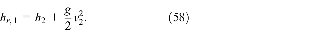
In simulations, the Newmark parameters are chosen as and to avoid numerical damping. The time step size is set to to to generate accurate results when using the second-order accurate Newmark- method. The simulation is stopped once the ball exceeds the initial distance of , let this time instant be denoted as . The first rebound height can then be computed from height and vertical velocity at time ,
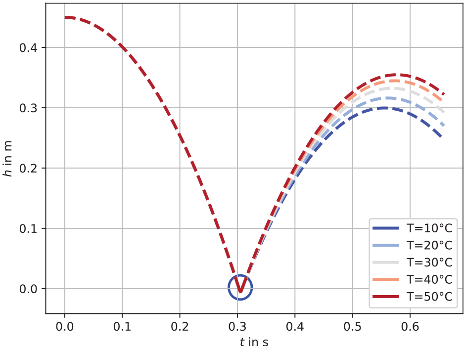
In Figure 8, the ball’s computed trajectory at different temperatures is presented, where the third order material characterization from Table 1 has been used. Five different ambient temperatures were chosen such that they cover the range of DTMA measurements. We use respectively, leading to the shifting parameters provided in Table 4.
Ball-drop trajectory, , using material data for from Table 1.
Shifting parameters for and different ambient temperatures .
in
10
20
30
40
50
2.4388
1.0
0.4387
0.1994
0.0959
1.0353
1.0
0.967
0.9361
0.9071
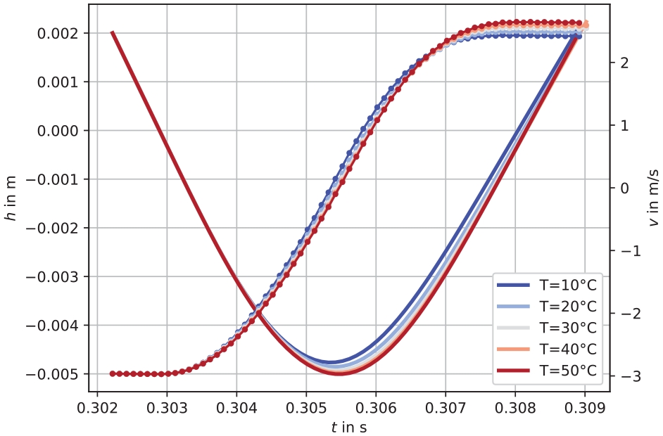
Free fall and rebound trajectories above height and respectively were generated analytically and are identified as dashed lines. Results of the actual simulation are highlighted in blue, and presented in detail in Figure 9. In addition to the trajectories, the ball’s vertical velocity is displayed for all temperatures. An increase in the rebound height for increasing temperatures can be clearly observed.
Impact trajectory (cmp. Figure 8), solid lines indicate the ball’s trajectory, dots mark its velocity.
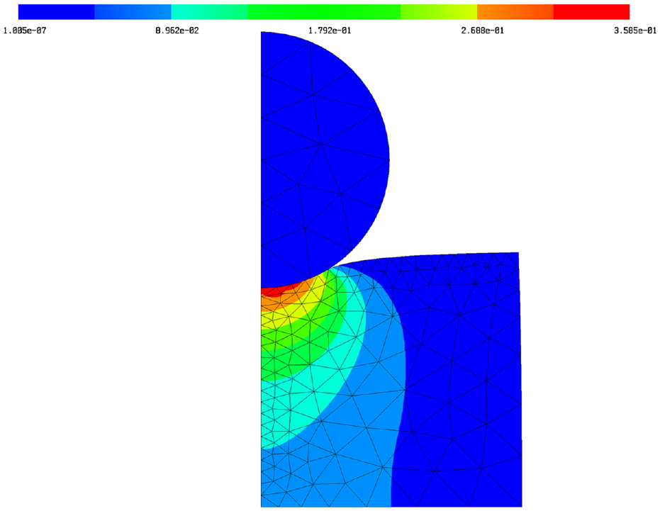
A closer look at the ball trajectory in Figure 9 shows that even for representing the stiffest sample, the indentation amounts to approximately 4.71 mm. The resulting compressive strain then corresponds to mean value of about 15%, and a peak value of around 35%. This clearly indicates large deformations, while an approximation by using the Neo-Hookean law is still justifiable. Figure 10 shows the according strain distribution at the time of maximum penetration of the ball. We visualize , being the compressive component of the strain tensor .
Strain distribution at maximum penetration state for , .
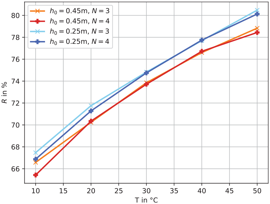
Damping properties of the material are often characterized through the rebound resilience or loss factor in the ball drop test, see Emminger et al. (2021). The loss factor is given by , often also referred to as . Both in the experiment and in the simulation, a number of parameters can be changed in order to better study the behavior. For example, the variation of the original height , the ball’s radius , the actual temperature as well as the order of the material model can provide suitable information.
Figure 11 shows the variation of the rebound resilience for different temperatures. From these results, we see that the third and fourth order material model lead to similar results; thus, a restriction to third order is viable to save computational effort. On the other hand, we observe that by decreasing the original drop height to 0.25 m, an increase in the rebound resilience is achieved. For increasing temperatures, the resilience increases independently of the drop height. At higher temperature, the material acts less viscous.
Rebound resilience comparison.
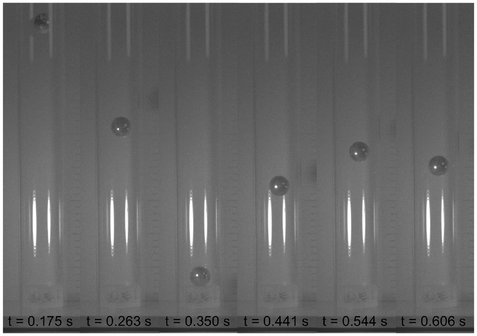
The computational results are compared to measurements taken in an according setup. For this purpose, an experimental setup has been designed, where the ball is released from an electromagnetic mount. A high-speed optical camera was used to track the trajectory of the ball, as shown in Figure 12. In this figure the six frames show the trajectory of the ball drop experiment. Video frames have been selected in such a manner that impact as well as maximum rebound height are visible. Indicated times do not correspond to simulation times but are computed according to the camera frame rate, being 1600 fps. More information on the setup and procedure of these measurements can be found in Preuer (2018). There, further samples were measured and compared using the same method.
Video frames of ball trajectory and impact.
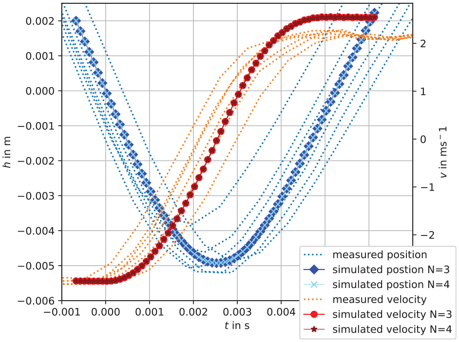
Care was taken to ensure that the surface of the sample was neatly powdered before each measurement in order to exclude possible friction and adhesion effects. Several of these measurements were carried out and are shown as dotted lines in Figure 13. The trajectories obtained from simulations, as shown in Figure 9, are compared to these measurement data curves around the time of impact. Again, third and fourth order show no difference for the height course and also the velocity.
Ball-drop measurements for , at .
It shows that the depth of penetration observed in simulation and experiment fit closely. In simulations, however, a higher rebound resilience of is observed as compared to in the experiments. Consistently, the velocity of the ball after impact is higher. It is not clear where the discrepancy originates from; certainly the friction-less contact model, the assumption of perfect rotational symmetry in displacements and also the rigid bedding of the PDMS specimen add to the computed rebound height, as dissipation is inhibited.
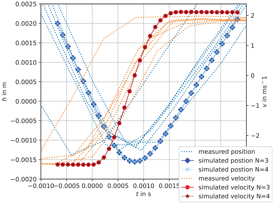
In a second set of experiments, a ball of radius was dropped again from the original drop height of , the ambient temperature is at . In Figure 14, corresponding measurements and simulation results are compared. Again, correspondence is observed for the indentation depth. Concerning rebound resilience and velocity after impact, the results fit better for this smaller ball. The rebound resilience in simulation is found at , whereas the measured rebound resilience was determined as
Ball-drop measurements for , at .
7. Conclusion
In the present article, we have introduced a thermodynamically consistent characterization for viscoelastic materials for modeling the behavior of the PDMS Sylgard 184. To determine the model’s parameters, a dynamical temperature mechanical analysis was conducted in a limited frequency range. The time-temperature superposition principle was used successfully to generate an extended frequency response. For this data, Prony-parameters based on the linear Wiechert model were identified using a non-negative least squares fitting algorithm. To verify this constitutive model, a mixed finite element model for rotationally symmetric problems was created. A ball-drop test setup was designed in order to conduct measurements on the rebound resilience for different ball sizes and drop heights. Data generated in the finite element simulation were then compared to optical tracking data from the experiment. Our numerical results match the measured data almost perfectly as far as the indentation depth is concerned. This also confirms the accuracy of linear parameters in a non-linear framework Rebound resiliences differ, however, as we observe less dissipation in computations than in experiments. To analyse these deviations in detail, the effects of friction-less contact and the imposed radial symmetry in computations need to be quantified in the future. Additionally, DTMA measurements in an even larger range of temperature may lead to a better characterization of the viscous behavior at high frequencies, which are certainly excited in a ball-drop test.
Footnotes
Declaration of conflicting interests
The authors declared no potential conflicts of interest with respect to the research, authorship, and/or publication of this article.
Funding
The authors received no financial support for the research, authorship, and/or publication of this article.
ORCID iDs
Mario Kunzemann
Leonhard K. Doppelbauer
Astrid Pechstein
Notes
Data availability statement
Data sharing not applicable to this article as no datasets were generated or analyzed during the current study.
References
1.
AriatiRSalesFSouzaA, et al. (2021) Polydimethylsiloxane composites characterization and its applications: A review. Polymers13(23): 4258.
2.
AskAMenzelARistinmaaM (2012) Electrostriction in electro-viscoelastic polymers. Mechanics of Materials50: 9–21.
3.
BorókALabodaKBonyárA (2021) Pdms bonding technologies for microfluidic applications: A review. Biosensors11(8): 292.
4.
BrinsonHFBrinsonLC (2015) Polymer Engineering Science and Viscoelasticity - An Introduction. Berlin; Heidelberg: Springer.
5.
CardosoCFernandesCSLimaR, et al. (2018) Biomechanical analysis of pdms channels using different hyperelastic numerical constitutive models. Mechanics Research Communications90: 26–33.
6.
ClarsonSDodgsonKSemlyenJ (1985) Studies of cyclic and linear poly(dimethylsiloxanes): 19. Glass transition temperatures and crystallization behaviour. Polymer26(6): 930–934.
7.
DeguchiSHottaJYokoyamaS, et al. (2015) Viscoelastic and optical properties of four different pdms polymers. Journal of Micromechanics and Microengineering25(9): 097002.
8.
DewimilleLBressonBBokobzaL (2005) Synthesis, structure and morphology of poly (dimethylsiloxane) networks filled with in situ generated silica particles. Polymer46(12): 4135–4143.
9.
DoghriI (2013) Mechanics of Deformable Solids - Linear, Nonlinear, Analytical and Computational Aspects. Berlin; Heidelberg: Springer Science and Business Media.
10.
EduokUFayeOSzpunarJ (2017) Recent developments and applications of protective silicone coatings: A review of pdms functional materials. Progress in Organic Coatings111: 124–163.
11.
EmmingerCÇakmakUDPreuerR, et al. (2021) Hyperelastic material parameter determination and numerical study of TPU and PDMS dampers. Materials14(24): 7639.
12.
FerryJD (1980) Viscoelastic Properties of Polymers. New York, NY: John Wiley & Sons.
13.
HauptP (2013) Continuum Mechanics and Theory of Materials. Berlin; Heidelberg: Springer Science and Business Media.
14.
KlompenEGovaertL (1999) Nonlinear viscoelastic behaviour of thermorheologically complex materials: A modelling approach. Mechanics of Time-dependent Materials3: 49–69.
15.
KnappANebelLJNitschkeM, et al. (2021) Controlling line defects in wrinkling: A pathway towards hierarchical wrinkling structures. Soft Matter17(21): 5384–5392.
16.
KrausMASchusterMKuntscheJ, et al. (2017) Parameter identification methods for visco-and hyperelastic material models. Glass Structures & Engineering2(2): 147–167.
17.
KunzemannMPechsteinAHumerA (2023) Thermodynamically consistent modelling of dielectric viscoelastic solids under finite strain. In: SaravanosDBenjeddouAChrysochoidisN, et al. (eds.) Proceedings of the X ECCOMAS Thematic Conference on Smart Structures and Materials, Patras, Greece, 5–7 July 2023, pp.1938–1949. Eccomas Proceedia. https://www.eccomasproceedia.org/conferences/thematic-conferences/smart-2023/9963
18.
LeeHMSungJKoB, et al. (2021) Modeling and application of anisotropic hyperelasticity of pdms polymers with surface patterns obtained by additive manufacturing technology. Journal of the Mechanical Behavior of Biomedical Materials118: 104412.
19.
LiWLiuFWeiL, et al. (2006) Synthesis, morphology and properties of polydimethylsiloxane-modified allylated novolac/4,4-bismaleimidodiphenylmethane. European Polymer Journal42(3): 580–592.
20.
LinIKOuKSLiaoYM, et al. (2009) Viscoelastic characterization and modeling of polymer transducers for biological applications. Journal of Microelectromechanical Systems18(5): 1087–1099.
LongKNBrownJA (2017) A linear viscoelastic model calibration of sylgard 184. Technical report, Sandia National Lab (SNL-NM), Albuquerque, NM.
23.
MieheC (2002) Strain-driven homogenization of inelastic microstructures and composites based on an incremental variational formulation. International Journal for Numerical Methods in Engineering55(11): 1285–1322.
24.
MieheCApelNLambrechtM (2002) Anisotropic additive plasticity in the logarithmic strain space: Modular kinematic formulation and implementation based on incremental minimization principles for standard materials. Computer Methods in Applied Mechanics and Engineering191(47–48): 5383–5425.
25.
MieheCRosatoDKieferB (2011) Variational principles in dissipative electro-magneto-mechanics: A framework for the macro-modeling of functional materials. International Journal for Numerical Methods in Engineering86(10): 1225–1276.
26.
NunesL (2011) Mechanical characterization of hyperelastic polydimethylsiloxane by simple shear test. Materials Science and Engineering: A528(3): 1799–1804.
TaylorCHoodP (1973) A numerical solution of the Navier-Stokes equations using the finite element technique. Computers & Fluids1(1): 73–100.
29.
TschoeglNW (2012) The Phenomenological Theory of Linear Viscoelastic Behavior - An Introduction. Berlin; Heidelberg: Springer Science & Business Media.
30.
TschoeglNWKnaussWEmriI (2002) The effect of temperature and pressure on the mechanical properties of thermo- and/or piezorheologically simple polymeric materials in thermodynamic equilibrium – a critical review. Mechanics of Time-Dependent Materials6: 53–99.
31.
ZamanQZiaKMZuberM, et al. (2019) A comprehensive review on synthesis, characterization, and applications of polydimethylsiloxane and copolymers. International Journal of Plastics Technology23: 261–282.
32.
ZhuDHandschuh-WangSZhouX (2017) Recent progress in fabrication and application of polydimethylsiloxane sponges. Journal of Materials Chemistry A5(32): 16467–16497.