
Abstract
Currently, it is challenging to obtain consistent values for the anisotropic electrical conductivity of fabric ply based thermoplastic composites. In this study, the anisotropic electrical conductivity of this type of material was obtained by combining six-probe voltage measurements with a numerical evaluation method to process the voltage measurements. The effect of probe distance and specimen dimensions on the test results was investigated. The measurements show low specimen to specimen variability and the obtained electrical conductivities agree with values obtained by the rule of mixtures and the two-probe measurement method. The conducted research shows that with one experiment, both the in- and the out-of-plane electrical conductivity of polymer composites reinforced with carbon fabrics can be reliably determined, simultaneously.
Introduction
Background
Carbon fibre reinforced polymer materials, referred to as composites, are more and more being applied in aerospace. The increasing demand for aircraft 1 drives the need for cost-efficient, high-rate production of composite structures. The last two decades have seen a growing trend towards the application of thermoplastic polymers as matrix material 2 owing to their short processing times, higher toughness and long shelf life. Since large composite structures are typically assembled from smaller components, joining techniques for composites have become a relevant research topic.
Mechanical fastening, a matured joining technology, 3 introduces problems for composites since the load carrying fibres are damaged and stress concentrations arise in the vicinity of the fasteners. Design rules have been developed to take these stress concentrations into account, unfortunately these design rules result in weight gains. 3 Adhesively bonded joints require no drilling operations and therefore, generally, weigh less compared to their fastened counter parts while creating a strong joint since stresses are distributed over large areas. However, to realise an acceptable final joint quality proper surface pretreatment is critical 3 and adhesive bonding is challenging for thermoplastic composites (TPC) due to the low surface energy of the thermoplastic polymer.
The use of a TPC enables joining separate components by fusion bonding, in which heat energy is utilized to melt the faying surface resin to achieve intimate contact and polymer chain diffusion and to accomplish the bonding process. In this technique, the healing capability of TPCs is utilised and the efficiency of the welded joint can approach the bulk properties of the adherents.3,4 A number of fusion bonding, or welding, techniques exist 5 differing in the way heat is generated. Ultrasonic welding, induction welding and resistance welding are currently being applied during the manufacturing process of commercial aerospace structures.3,4
With induction welding, the heat is generated as a result of energy losses of electric currents running through the electrically conductive fibres of the composite. The electric currents are induced by the change of the magnetic flux density created by an alternating electric current in a coil located in the vicinity of the composite. The existence of closed electric loops within the conductive material is a necessary condition for induction to occur. In thermoplastic composites with a carbon fibre fabric reinforcement, the specific type of composites of the present study, the fibre bundles are able to form a closed electric loop either by direct contact or by indirect contact when separated by a small amount of the dielectric polymer.
Different heating mechanisms have already been identified in earlier studies on induction heating of composites with a carbon fibre fabric reinforcement.6,7 These mechanisms can be distinguished in i) heating by Joule losses along the fibre bundles; ii) heating by contact resistance at junctions between fibre bundles; and iii) heating by dielectric hysteresis at the fibre bundle junctions where fibres are separated by a layer of thermoplastic polymer.6,8–10 These three mechanisms are depicted in Figure 1. The amount in which each mechanism contributes to the total heat generation depends on the electrical properties of the constituents in a ply as well as on the architecture of the fabric. Mitschang et al.
11
showed that direct fibre contacts are formed at the junctions of the interlacing fibre bundles in a fabric ply. The adjacent plies in a laminate are likely to be in direct contact, although the extent of contact is unknown. Schematic overview of the heating mechanisms in induction heating of thermoplastic composites with woven reinforcement.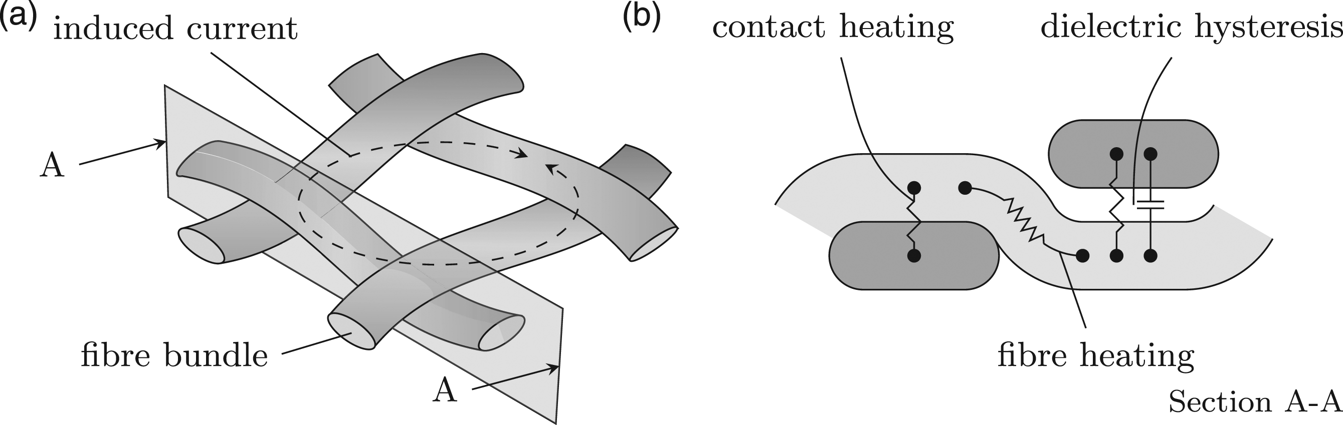
Currently, the process window definition of an induction welding process in industrial practice in which fabric-ply based TPCs are joined, 12 largely relies on empirical methods. Once the process window is defined, high repeatability of the weld quality is obtained by proper process control. Nevertheless, insufficient fundamental understanding of the process prevents properly anticipating (and, if needed, mitigating) the effect of a change somewhere in the process chain on the weld quality. Moreover, an accurate predictive capability accelerates the specification of induction welding process parameters which is key in reducing cost and turnaround time for larger thermoplastic composite parts.
The process window could be defined using existing numerical simulation software, e.g. COMSOL Multiphysics 13 or Abaqus, 14 in which electromagnetic and thermal models are coupled. The outcome of these models is highly dependent on the input material property data, especially on the electrical conductivity matrix. Currently, reliable data on electrical conductivities are hardly available for most composite materials due to little consensus regarding a standardised method to characterise this property.
Publications in which the electrical conductivities of TPCs, with a carbon fibre fabric reinforcement, are required for induction heating simulations are using either anisotropic electrical conductivities9,11,15–21 or an equivalent electrical conductivity.22,23 While the former approach allows for the prediction of inductive heating of arbitrary laminate lay-ups and arbitrary coil configurations, the application of the latter approach is limited to bidirectional and isotropic structures22,23 with an axisymmetric coil geometry 23 and a fibre volume fraction φf of at least 0.6523. In this study, preference is given to a generically applicable method, hence the equivalent conductivity method is not considered in this study.
The applied in-plane anisotropic electrical conductivities in the considered studies were determined by applying the rule of mixture, according to


Overview of applied electrical conductivities at fabric ply level, normalised to a φf of 0.50, in published studies on simulation of heating by induction of composite materials with a carbon fibre fabric reinforcement.
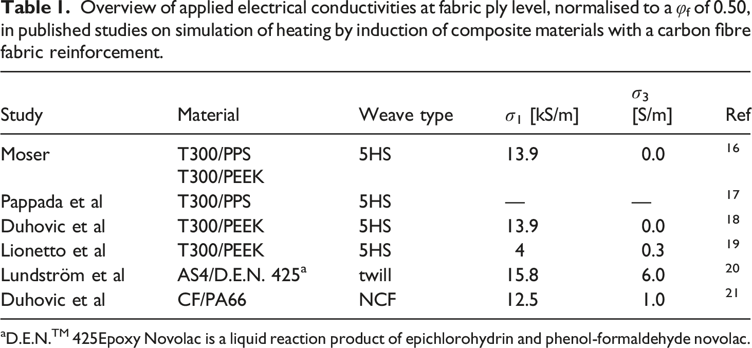
aD.E.N.TM 425Epoxy Novolac is a liquid reaction product of epichlorohydrin and phenol-formaldehyde novolac.
Several measurement methods are available to determine the electrical conductivity of an anisotropic material. The methods can be divided in uniform and non-uniform current density methods. Figure 2 provides a schematic overview, intended to show the basic principles of the measuring methods, of a number of methods applied in previous studies; the practical application of the electrodes to the specimens has been omitted from this schematic overview. Schematic representation of the found electrical conductivity measurement test set-ups: (a) voltage measurements occur at contact surfaces; (b) voltage measurements using line contact probes or point contact probes; (c) voltage measurements occur at contact surfaces; (d) voltage measurements by means of point probes; (e) voltage measurements by means of line contact probes.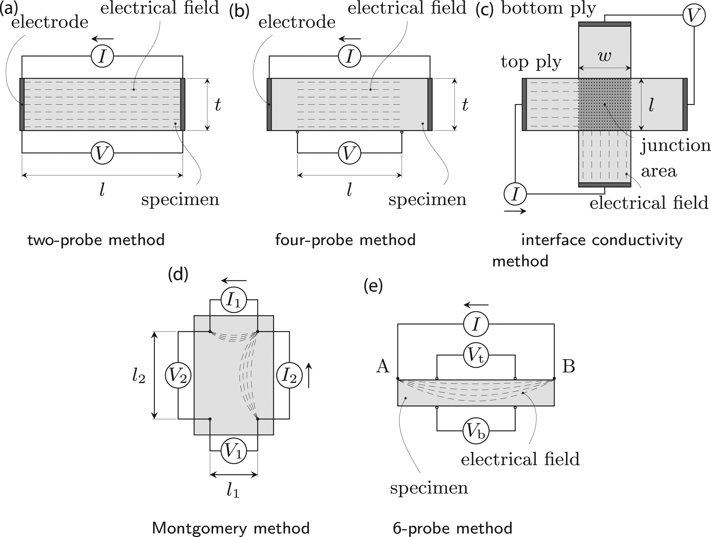
In most studies where the electrical conductivity of a TPC is investigated, this property is characterised by a uniform current density method. A well known uniform current density method is the two-probe method of which a schematic overview is depicted in Figure 2(a). Schulte et al., Kim et al. and Todoroki et al.7,25,26 applied this method in their studies. In this method, a direct current I is applied by electrodes which are installed at two opposing parallel end faces of the specimen. The aim is a uniform distribution of the current density across a specimen’s cross-section, depicted in the figure by the equidistant dashed lines. The measured voltage drop between the electrodes, V, over distance, l, being the specimen’s length, is used to calculate the conductivity by applying Ohm’s law,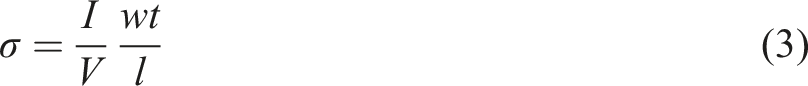
The four-probe method, shown in Figure 2(b), is generally applied24,27–29 to determine a composite’s in-plane electrical conductivity. Similar to the two-probe method, a direct current, I, is applied by electrodes installed at two opposing parallel end faces of the specimen. The voltage drop is measured using extra probes which are positioned between the electrodes through which the current is applied. Both point contact probes 29 as well as line contact probes 24 are used. The measurement probes eliminate the electrode resistance in the measurements. The current is assumed to be uniformly distributed between the voltage measurement probes making this method less susceptible for an inadequate contact quality between electrode and specimen and therefore the contact surface preparation might become less laborious compared to the surface preparations needed in the two-probe method. The measured voltage drop, V over distance l, is used to calculate the conductivity by applying Ohm’s law, equation (3).
Wang et al.
30
and Guerrero et al.
31
investigated the electrical conductivity of the interface between the plies of a composite laminate. In their method, schematically shown in Figure 2(c) and (a) uniformly distributed current over the junction area is assumed. The interface’s contact conductivity, σc, is calculated by,
This method requires an evenly distributed current over the width of the electrodes to which the current is applied.
Non-uniform current density methods generally assume a specific distribution of the current density in the specimen. A well-known method to determine a material’s anisotropic electrical conductivity is the so-called Montgomery method 32 and is schematically shown in Figure 2(d). The anisotropic electrical conductivities are obtained by specific voltage measurements between the point probes combined with the specimen dimensions. 32 This method is, in the case of composites, only suitable to characterise the in-plane anisotropic electrical conductivities.
In a more recent study, performed by Hart and Zhupanska, 33 the six-probe method, shown in Figure 2(e), has been investigated using uni-directional composites. In this method, an electrical current is applied through a line contact at positions A and B in the figure and voltages are measured in between these positions. The line contacts makes surface pretreatments, such as needed in the discussed uniform current density methods, superfluous. This is specifically the case when this method is applied to characterise the anisotropic electrical conductivities of carbon fabric reinforced composites, the fabric’s fibre bundles oriented in the specimen’s width direction take care of the distribution of the applied electrical current in this direction. However, due to the non-uniform current density distribution in the specimen’s thickness direction, the determination of the anisotropic electrical conductivities from the voltage measurements becomes more complex compared to the uniform current-density methods.
The electromagnetic eddy current measurement method is an example of another non-uniform current density method. Application of this method is reported by Mook et al. 34 and Cheng et al. 35 to be used for qualitative comparisons between composite materials rather than for quantitative purposes. More recently, Lundström et al. 20 combined rule of mixtures, equation (2), to determine σ1, with eddy current measurements to characterise σ3. To derive the out-of-plane electrical conductivity from the eddy current measurement data, the inverse numerical method, as described by Mizukami and Watanabe, 24 was applied.
The objective of the current research is to develop and demonstrate a reliable method to measure the anisotropic electrical conductivity of carbon fibre fabric reinforced thermoplastic composites, without being dependent on delicate contact surface preparations. The initial concept in the study is the six-probe method which was identified as the most practical to ensure a sufficient contact quality between specimen and probe. As mentioned before, the six-probe method does not require any surface pretreatment since the well-defined line contact in combination with the fabric’s fibre bundles in the specimen’s width direction are utilised to ensure the transverse homogeneity of the current distribution in the specimen’s width direction. More importantly, one experiment determines both the in- and the out-of-plane electrical conductivity of polymer composites reinforced with carbon fabrics, simultaneously.
Theory
In this section, the six-probe measurement method is outlined followed by a numerical method to derive the anisotropic electrical conductivities from the measured voltages.
The six-probe voltage measurement method
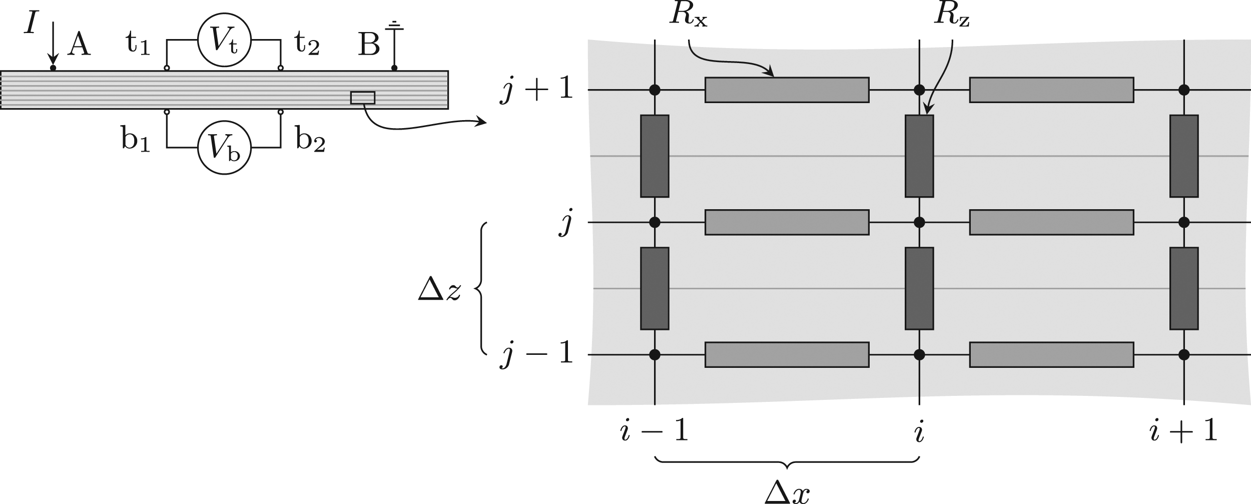
In the six-probe method, an electrical current is applied at the top surface of a specimen over a distance L from point A to point B, as depicted in the two-dimensional schematic representation in Figure 3. As a result of the applied current between point A and B, a non-uniform electrical field density is generated in the specimen, shown by the dashed lines. The voltage drop measured over distance l at the top surface Vt is not equal to the measured voltage drop over the same distance l at the bottom surface Vb. The distribution depends on the distance L, the thickness of the specimen, and the in- and out-of-plane specific electrical conductivities of the specimen. For the herein presented method and the materials to be characterized, it can be assumed that the electrical current is evenly distributed over the width of a specimen due to the presence of the fabric’s fibre bundles in this direction. A cross-sectional view of a specimen undergoing a six-probe measurement.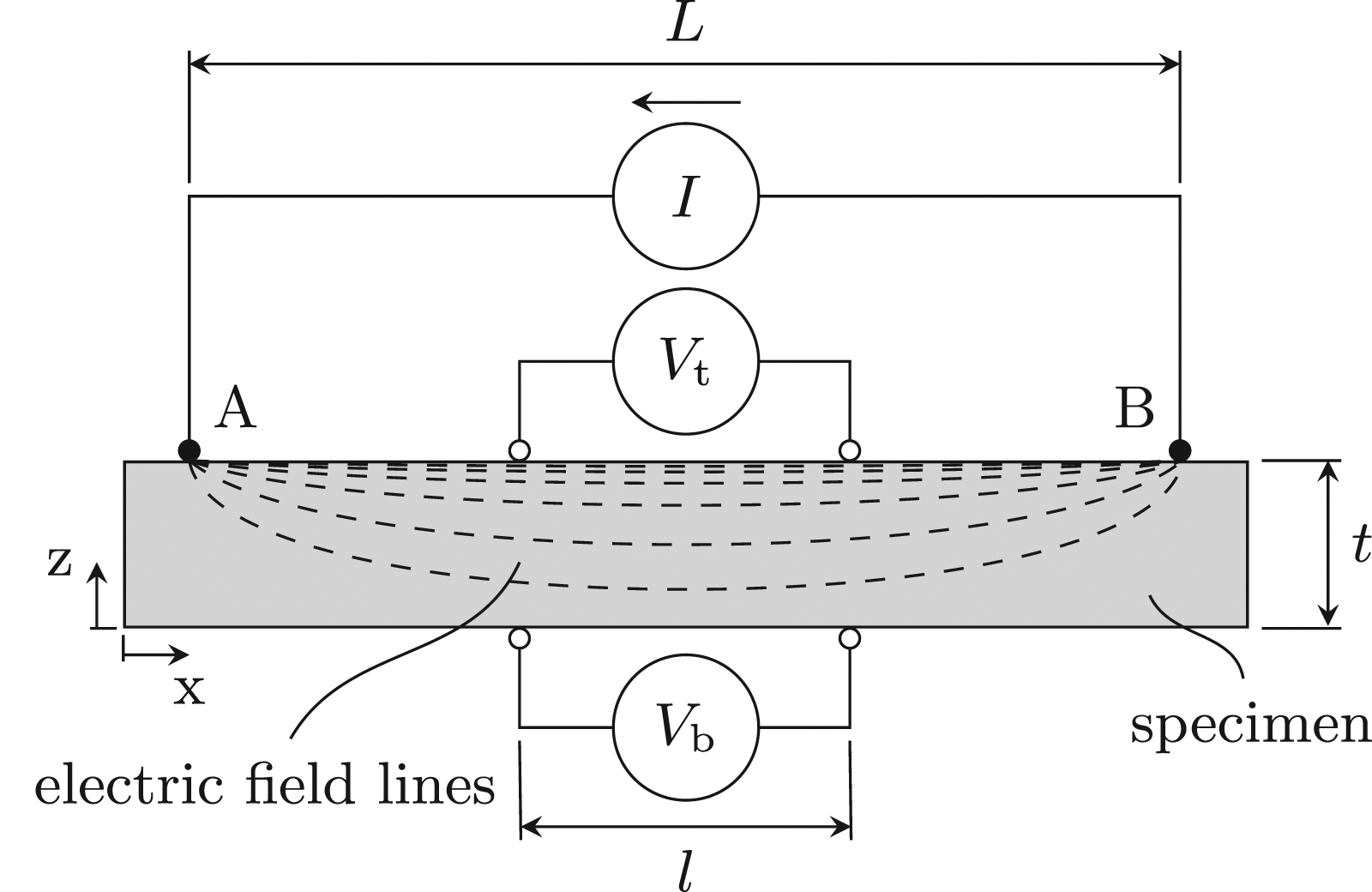
Numerical model description
Hart and Zhupanska
33
developed a procedure to derive the anisotropic electrical conductivities from six-probe measurements on unidirectional composites. Their procedure expands upon work performed by Busch et al.,
36
in which an analytical approximation is presented to measure the electrical conductivity of strongly anisotropic single crystals using the six-probe method. This analytical approximation can be obtained by solving the differential equation describing the two-dimensional potential distribution V(x, z) in the specimen during a six-probe experiment,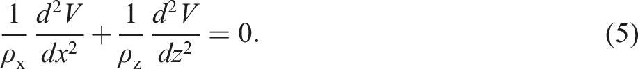
An appropriate solution is given by expansion

Using the measured voltages Vt and Vb at the known locations one obtains from the ratio Vt/Vb,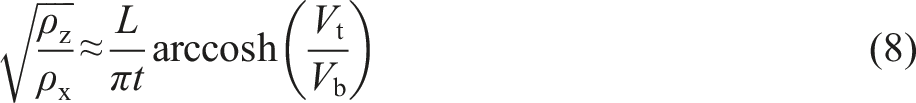
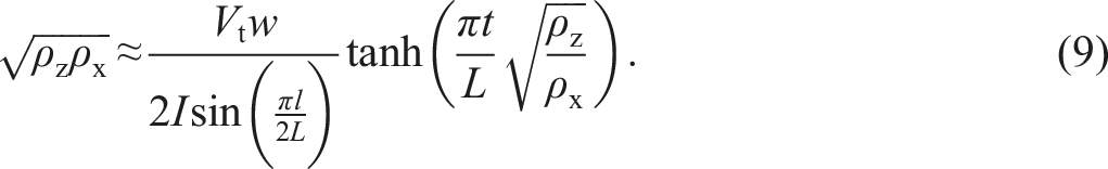
Dividing the result of equation (9) by the result of equation (8) gives ρx; multiplication of the result of equation (9) by the result of equation (8) gives ρz.
If this approach were to be applied to characterise the electrical conductivities of a TPC, this would be limited to lay-ups in which all plies are oriented. To be able to measure the electrical conductivities of arbitrary lay-ups (e.g. quasi-isotropic) it was decided to develop a straightforward numerical approach in which more than one ply orientation in the lay-up can be analysed to derive the specific electrical conductivities from six-probe measurements. Our results include a comparison of the conductivity values obtained using the numerical approach with values obtained using Busch’s method.
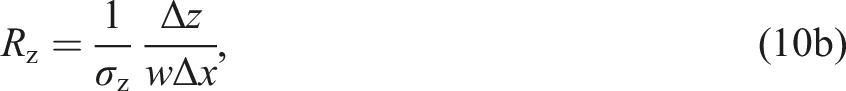
In the numerical model, the specimen is considered as a number of stacked plies in which each ply is regarded as a number of resistances in series, Rx, shown in Figure 3. The plies are electrically connected to each other by out-of-plane resistances, Rz. Rz represents all resistances in the through-thickness direction, thus intra ply, inter ply and the constituents. Consequently, a so-called resistor grid is created as schematically shown in Figure 4, in which Δx represents the distance between the nodes in x-direction and Δz the distance between the nodes in z-direction. The values of Rx and Rz are calculated according to Schematic overview of the numerical representation of the electrical conductivity of a specimen.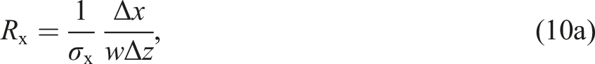
A general nodal analysis is performed to compute the unknown voltages in this grid, after which the estimation of σx and σz is improved by means of minimizing the error between the measured voltages Vt and Vb, and the calculated voltages at the corresponding nodes in the grid. An extensive explanation of the general nodal analysis can be found in, 37 nevertheless a description is briefly summarised here for convenience together with the minimisation process.
To determine the unknown voltages, Kirchhoff’s current law is combined with Ohm’s law to formulate an objective function 


The unknown nodal voltages are obtained by minimising Flowchart of the numerical method to determine the anisotropic electrical conductivities from six-probe voltage measurements.
The objective functions
Experimental work
Test matrix for experimental assessment of the six-probe method. The dimensions t, w, l and L are defined in Figure 3. The fibre volume content, φf, was 0.51 ± 0.01. Per configuration, six specimen were tested.
Materials
Properties of fibre, neat resin and woven fabric prepreg as specified in the manufacturer’s data sheet.
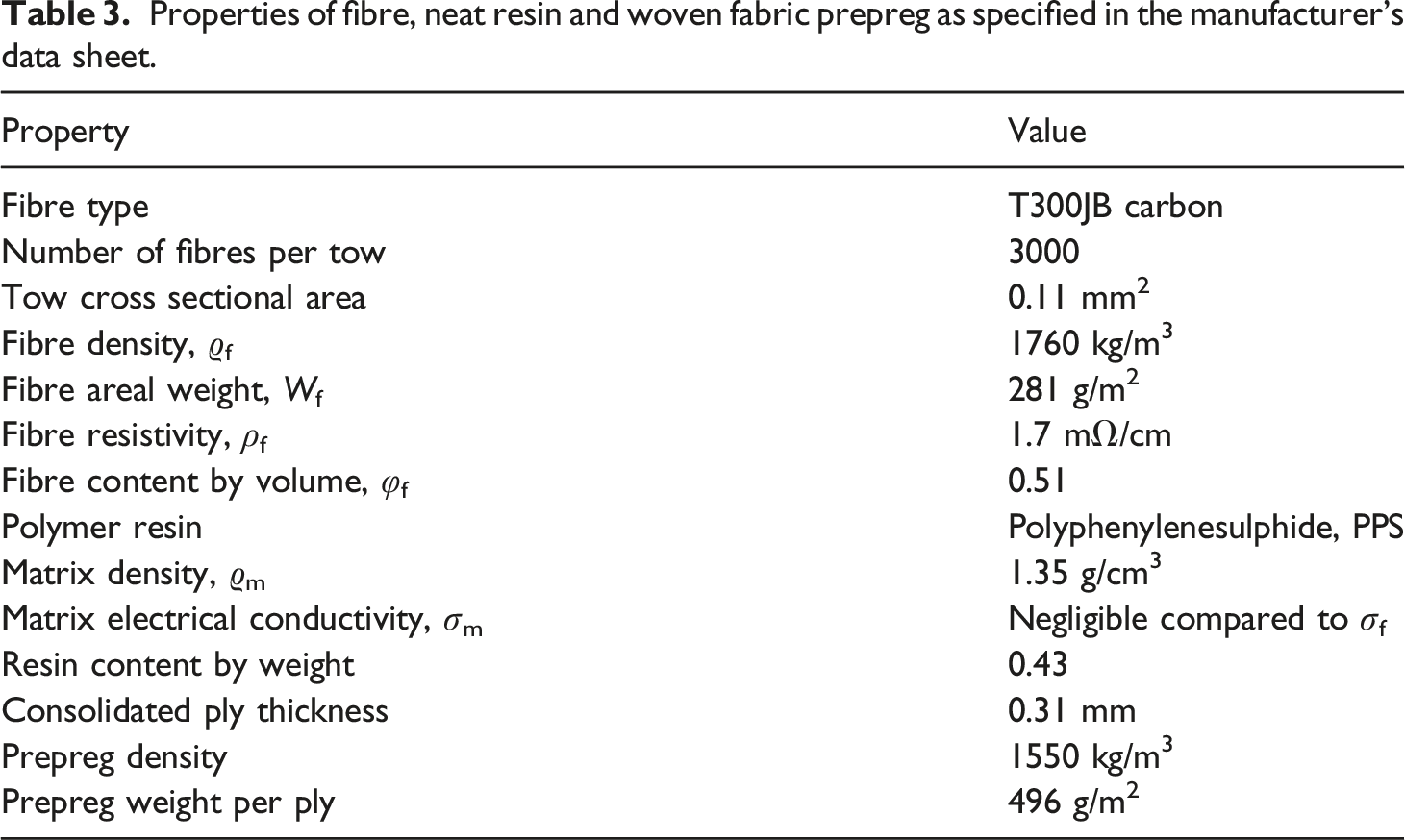
The laminates were consolidated using a picture frame mould of 305 × 305 mm2 in a static press. The mould was heated at a rate of 10°C/min. To a temperature of 312°C, kept at this temperature for 10 min and subsequently cooled down to room temperature at a rate of 5°C/min. The laminates were consolidated at a pressure of 10 bar. The resulting fibre volume content of the C/PPS composite laminates amounted 0.51 ± 0.01, which was calculated according to.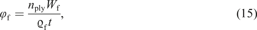
The six-probe measurement set-up
A fixture was developed to perform the six-probe experiments, which is shown in Figure 6. The fixture consists of a stainless steel (AISI 304L) base plate to which four clamps can be attached at defined positions. A schematic cross-sectional view of a clamp is shown in Figure 6(a). A line contact between the probes and the specimen was pursued to generate a 2-dimensional electrical field as assumed in Figure 3. This line contact also provides a high contact pressure to improve the contact between probe and specimen and accurate dimensions of L and l. The electrodes are copper plates with a designed knife edge with a slope angle of 45°, which have not been deburred in order to obtain the smallest possible tip radius (the obtained tip radius was 10–50 µm) to create a line contact over the complete width of a specimen. To electrically insulate the electrodes from the metal components which is also thermally resistant, micanite, supplied by Kuhne Industry (Nijkerk, the Netherlands) was chosen. Micanite is a commercially available plate material consisting of approx. 90% micapowder and 10% silicone or epoxy binder material. The guiding rods in Figure 6(b) provide for the vertical guidance of the upper half of the clamps enabling accurate and reproducible in-plane positioning. Overview of the six-probe test fixture, the cross-sectional views of one of the clamps shows the applied materials in the fixture; a) cross section side view; b) cross section front view; c) overall overview of the six-probe test set-up, depicted probe distances in the picture are L = 240 mm and l = 120 mm.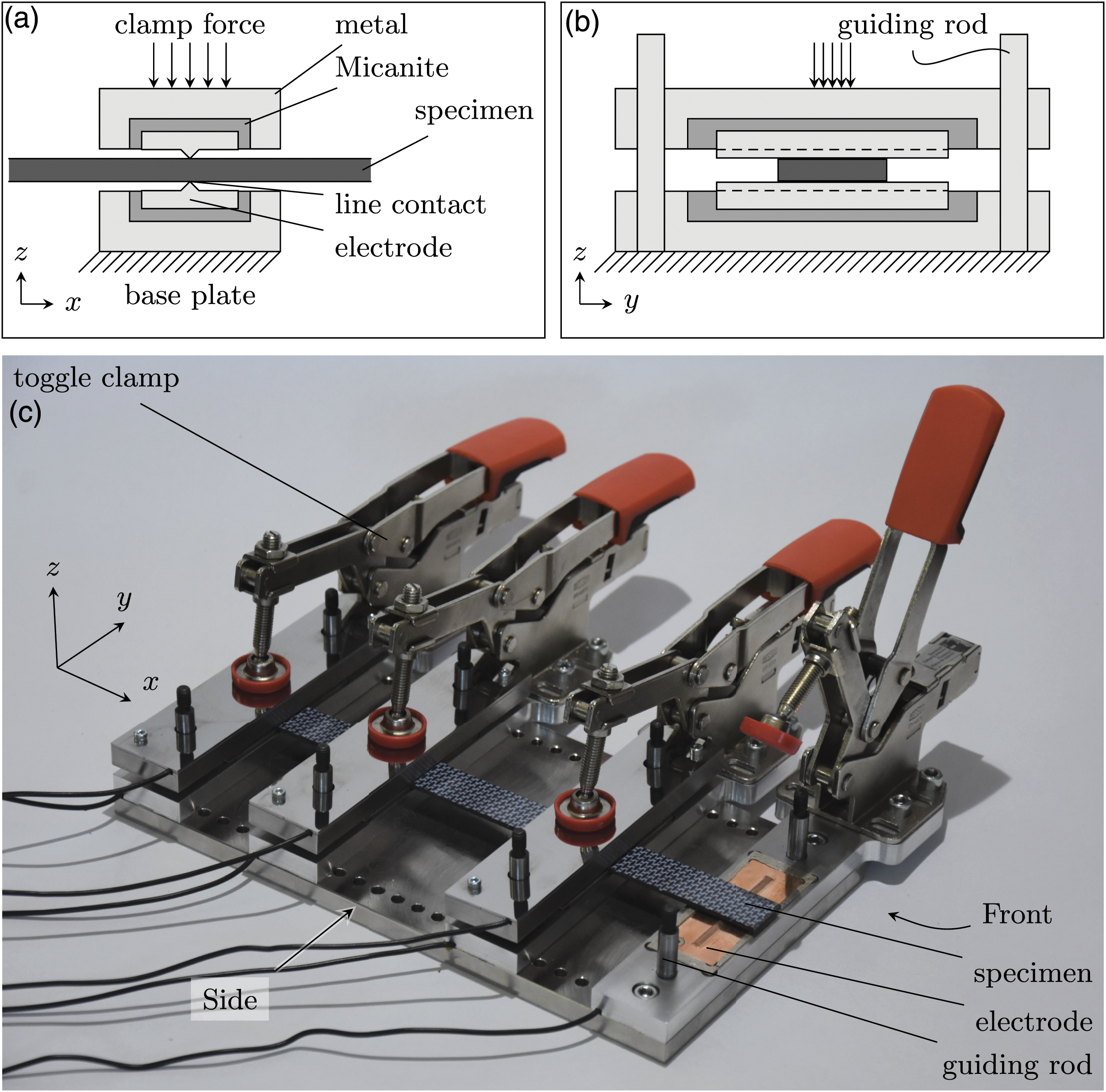
The clamping force is provided by commercially available horizontal toggle clamps (Bessey STC-HH70) which are able to provide a clamping force up to 2500N, according the specifications. The adjustable force was set to the maximum which has not been measured separately. As the contact resistance at the measurement probes does not play a role in the six-probe measurements, it is assumed that this clamping force is sufficient to obtain consistent voltage measurements.
A direct current (DC) Lab power supply was used in combination with a TiePie HS6D-100 differential oscilloscope data acquisition system. Per experiment 5000 data points were generated over a time period of 50 ms at a sampling rate of 100 kHz. An electrical current of 200 ± 5 mA was applied in all six-probe experiments. The specimens did not show heating at this amperage, avoiding contingent thermal effects.
The two-probe measurement set-up
The validation of the σz values obtained by six-probe measurements consisted of a comparison with σz values retrieved from two-probe measurements. A DC Lab power supply was used to apply a current, I, of 150 ± 5 mA to flat 25 × 25 mm2 copper electrodes in between which a 15 × 15 mm2 specimen was clamped with a force of F = 1500 ± 25N. The clamp force was applied by a loading screw to a movable holder in which the upper electrode is placed. The guiding rods in Figure 7 provide for the vertical guidance of the upper electrode holder to ensure the in-plane positioning of the upper electrode. Electrically isolating material (Micanite) was placed between the electrode holders and the electrodes. The clamping force was measured using a load cell. An Arduino Uno was used to collect the data from the load cell and to measure the voltage drop. The specimens undergoing two-probe measurements required a surface pretreatment to ensure sufficient contact quality between electrode and specimen. The preparation of the specimen’s contact surfaces consisted of machine polishing for 3 min with a Struers Tegramin 30 at a rotation speed of 80 rpm. and a force of 20 N. SiC Foil 2000 grit was used with water as coolant medium. Schematic overview of the two-probe test fixture; (a) front view, (b) side view.
Experimental results
A typical six-probe test result is shown in Figure 8. The figure shows the voltage drop measured in an experiment where a 200 mA electrical current was applied to a 20 mm wide [(0,90)]6s specimen. The current was applied over a distance, L, of 240 mm and the distance, l, between the measurement probes was 160 mm. Both of the voltage drop measurements at the top and at the bottom surface of the specimen as well as their averages are represented, respectively 43.1 ± 5.9 mV and 20.8 ± 3.8 mV. The noise shown was considered acceptable and hence averaging the data points obtained during a measurement was applied as a data reduction method. Typical test result of a [(0,90)]6s specimen; I = 200 mA, w = 20 mm, L = 240 mm, l = 160 mm, t = 2.47 mm.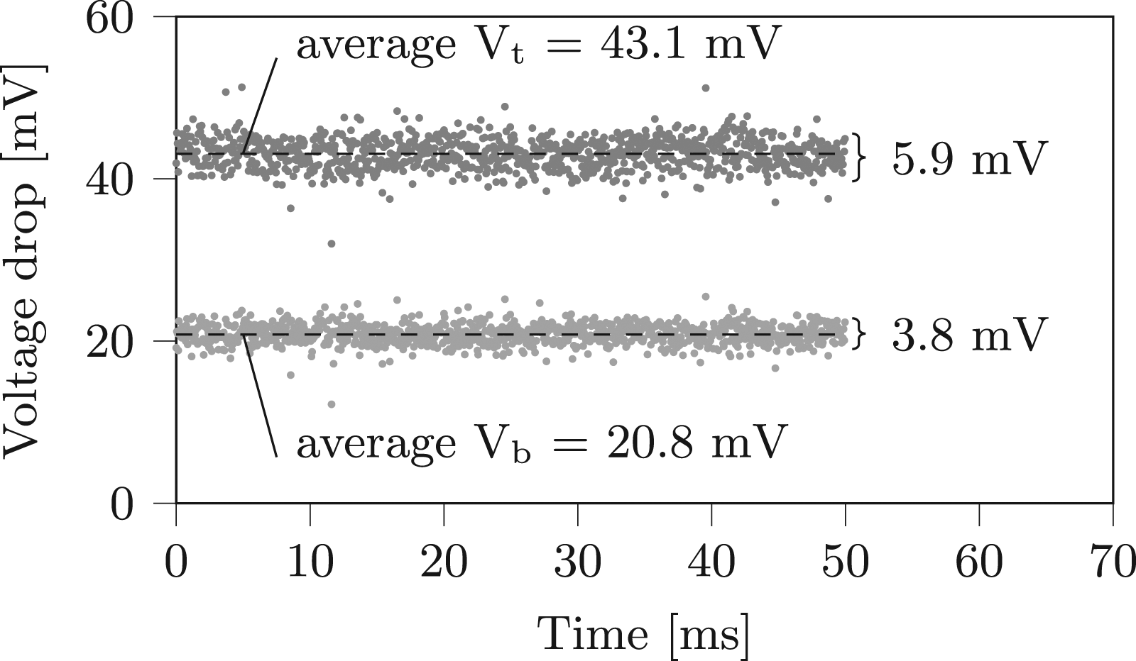
Numerical model considerations
The distances between the nodes, explained in the numerical model description and shown in Figure 4, were determined based on a convergence study on a four ply specimen with the lowest value for L, 120 mm. The convergence study showed that 24 elements over L could sufficiently describe the gradient of the voltage potential between the current probes. Duplicating this amount to 48 elements did not provide a change larger than 1% of the electrical conductivities. Since homogenised σx and σz values are determined, Δz does not have to agree with the ply thickness, however the number of elements in thickness direction were set to agree with the number of plies in the laminate since the convergence study showed that decreasing Δz with a factor of 2 affected the electrical conductivity by 3%.
Results and discussion
The test data, provided in the appendix is discussed in this section for each investigated topic shown in Table 2. The graphs shown in this section present the mean values and the standard deviations provided in the tables in the appendix. Each mean value and standard deviation in the tables are obtained from experiments on six specimens.
The influence of the width and thickness of the specimen on the electrical conductivities
The voltages in the six-probe measurements of set A in Table 2 are presented in Figure 9. The specific data of these experiments is provided in Table A1 in the Appendix. Figure 9 shows low specimen to specimen variability and linearly increasing values of V with increasing values of 1/w as can be seen by the linear dashed lines provided as guide for the eye. The most apparent finding to emerge from the proportionality analysis is that the electrical current is properly distributed in the width direction at the positions of the voltage measurement probes. This justifies a 2-dimensional representation of the electrical current distribution such as applied in the presented numerical method to derive the electrical conductivities from six-probe measurements in this case. Overview of the voltage measurements in which the influence of w and t is investigated, set A in Table 2. (a) top surface, (b) bottom surface.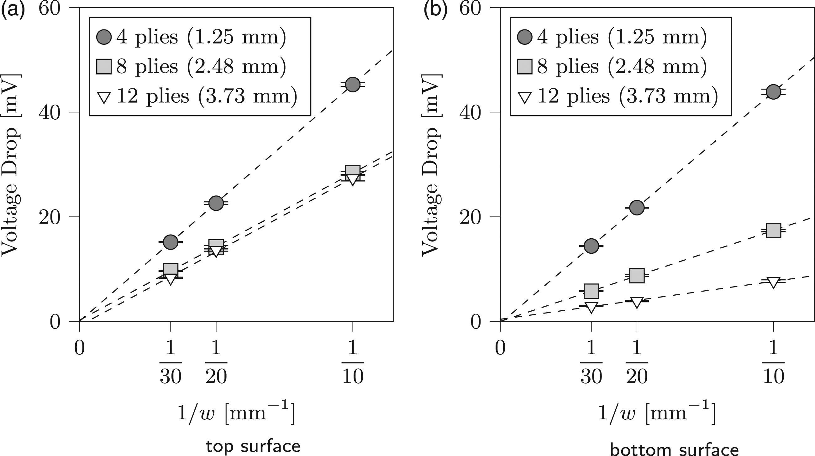
Figure 10 shows low specimen to specimen variability as well, however a non-linear relation between voltage drop and laminate thickness exists. Overview of the voltage measurements of set A in which the influence of w and t is investigated. A non-linear relation between V and t is observed. (a) top surface, (b) bottom surface.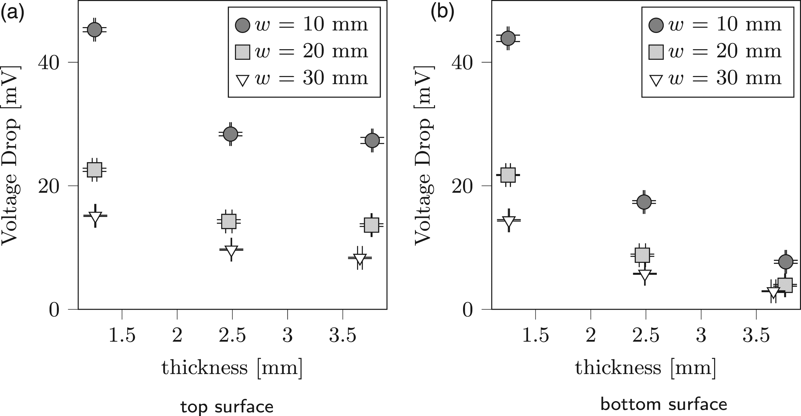
The voltages in the six-probe measurements were interpreted using the previously described numerical method to obtain the in-plane electrical conductivities, shown in Figure 11(a), and the out-of-plane electrical conductivities, shown in Figure 11(b). The σx values show high consistency independent of the number of plies in the laminate and the specimen width. This is in line with the expected electrical conductivity σx of 15.00 ± 0.29 kS/m, calculated using equation (2), and (15) and the data provided in Table 3. The σz values show less consistency, σz varies between 9.3 ± 0.3 and 19.0 ± 4.8 S/m. Moreover, for an increasing number of plies, a decrease of these values seems to be applicable which could indicate the existence of a thickness-related electrical resistance phenomenon, this can currently not be explained by e.g. differences in production since all laminates from which the specimens were taken underwent the same consolidation cycle. However, the obtained σz values in this set all fit within the characterised range obtained on a large proprietary dataset on the same material, this is represented by the gray area in the background of Figure 11(b), hence a thickness dependency cannot be concluded based on the limited amount of tested specimen in the present work. Overview of the electrical conductivities of set A in which the influence of w and t (represented in the Figure by the number of plies) is investigated. The gray area in the background of Fig. b represents proprietary conductivity data. (a) in-plane, (b) out-of-plane.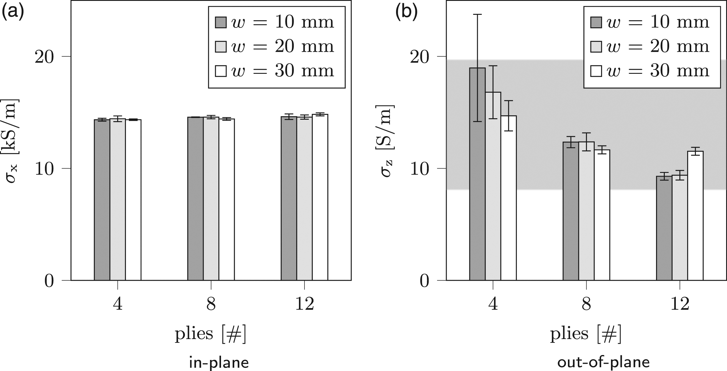
The σz values, smaller by a factor of thousand than the σx values, also show a higher relative variability of 8.2% compared to the relative variability of 1.0% for the σx values. The relative variability increases with decreasing number of plies. The higher relative variability for the σz values could be explained by the specimen to specimen variation. The determination of σx is dominated by the Vt measurement, while the determination of the σz value is dominated by the difference between Vt and Vb, while the absolute variability in Vt − Vb remains similar to the absolute variability in Vt. This is visualized in Figure 12 where Vt − Vb is shown alongside the Vt values of Figure 11(a), each on their own scale. This consideration shows that, in order to obtain low variability in the σz values, the width of a specimen should increase with decreasing thickness. Representation of the voltage measurements to visualize the high relative variability in Vt − Vb compared to the Vt measurements causing the high relative variablility in the σz values. (a) Vt, (b) Vt−Vb.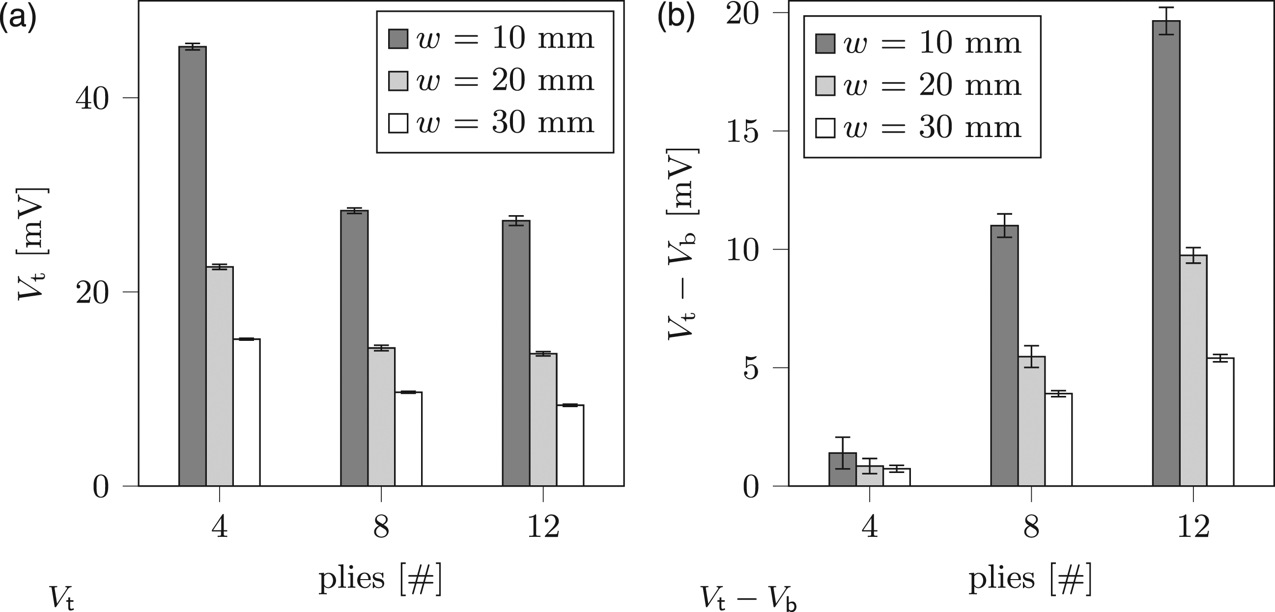
The influence of the probe distances on the electrical conductivities
The voltage measurements of set B and C are presented in Figure 13 for both the experiments with a constant L/l-ratio as well as the experiments in which l has been varied while L was kept constant at 240 mm. The voltage data shows low specimen to specimen variability. Overview of the voltage measurements to investigate the influence of l and L; second order polynomials were applied as a visual aid for the regression lines. (a) Set B, constant l/L-ratio, (b) Set C, varying l/L-ratio.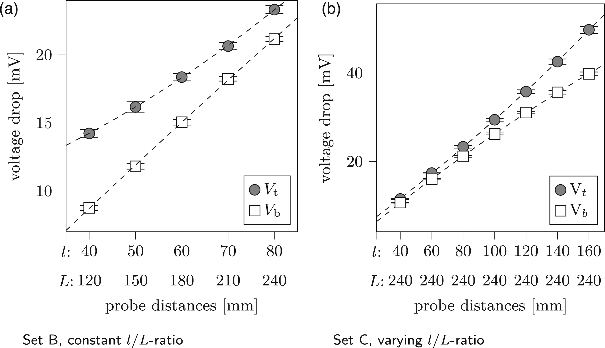
The behaviour between probe distance and measured voltage depends on the l/L ratio. A small l/L ratio means that the measurement probes are not in the vicinity of the current introduction positions (points A and B in Figure 3), consequently the voltage measurements become less affected by the current introduction and shows a direct proportionality with the probe distance l. The opposite applies for a large l/L ratio, in that case the voltage measurements become affected by the current introduction and shows a higher order correlation with the probe distance. In Figure 13, second order polynomials are applied as visual guide for the regression lines, however it is more likely that a closed form description is more complex. The conductivity values of these experiments are provided in Tables A2 and A3 in the Appendix for the experiments with a constant L/l-ratio and for the experiments with a varying L/l-ratio, respectively. As can be observed from these experiments, the anisotropic electrical conductivities do not show significant dependency on the probe distance configurations tested.
Validation of the numerical method to determine the electrical conductivities from six-probe measurements
The electrical conductivities obtained from the six-probe voltage measurements in combination with the present numerical method is assessed in this section. The six-probe voltage data used in this section is provided in Table A4 in the Appendix alongside the numerically determined electrical conductivities. The two-probe data used in this section is provided in Table A5 in the Appendix.
The numerically determined σx values are compared with the σx values obtained, based on the same six-probe voltage data, using the analytical approach by Busch et al., 36 equations (8) and (9), and with the calculated σx of 15.00 kS/m, previously obtained using the rule of mixtures.
The numerically determined σz values are compared with the σz values obtained using the analytical approach by Busch et al.
36
and with the σz values obtained from the two-probe measurements of set E. The two-probe data is presented in Figure 14 by means of the measured resistances, R = V/I. Figure 14 is depicted in terms of resistances since the intercept at t = 0 mm of 62 ± 23 mΩ, represents the average contact resistance between electrode and specimen. The average σz value was derived being 19.2 ± 0.7 S/m using the gradient R/t = 231 ± 9 mΩ/mm and the specimen’s cross-sectional area of 15 × 15 mm2. Overview of the two-probe voltage measurements of set E, performed to determine σz, to validate the numerical method.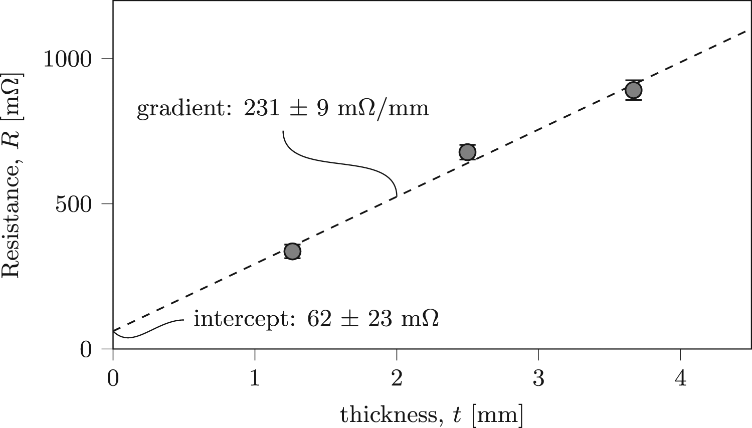
The anisotropic electrical conductivities obtained in experiment sets D and E, using all the different methods described above are presented in Figure 15. This overview shows high consistency in the σx values, regardless the applied analysis method. The overview of the σz values in Figure 15(b) does show a discrepancy between the approach by Busch et al. and the other two methods, especially for the 4-ply specimens. Due to the quite quickly converging σz values using Busch’s method towards the σz values obtained using the other two methods for an increasing number of plies, it is presumed by the authors that the limited number of terms (n = 1) considered in equation (6) is inadequate for a sufficiently accurate description of the potential distribution V(x, z) when the difference between Vt and Vb is small, which is the case for low ply numbers. However, to check this assumption, complex mathematical derivations are needed (if even possible) which are beyond the scope of this work. The σz values obtained using the six-probe method in combination with the numerical method shows consistency with the σz values resulting from the two-probe measurements being 19.9 ± 1.2 S/m and 19.2 ± 2.0 S/m respectively. (a, b) Comparison of electrical conductivities obtained from two-probe and six-probe measurements in combination with the numerical method and the method proposed by Busch. The gray area in the background of Fig. b represents proprietary conductivity data.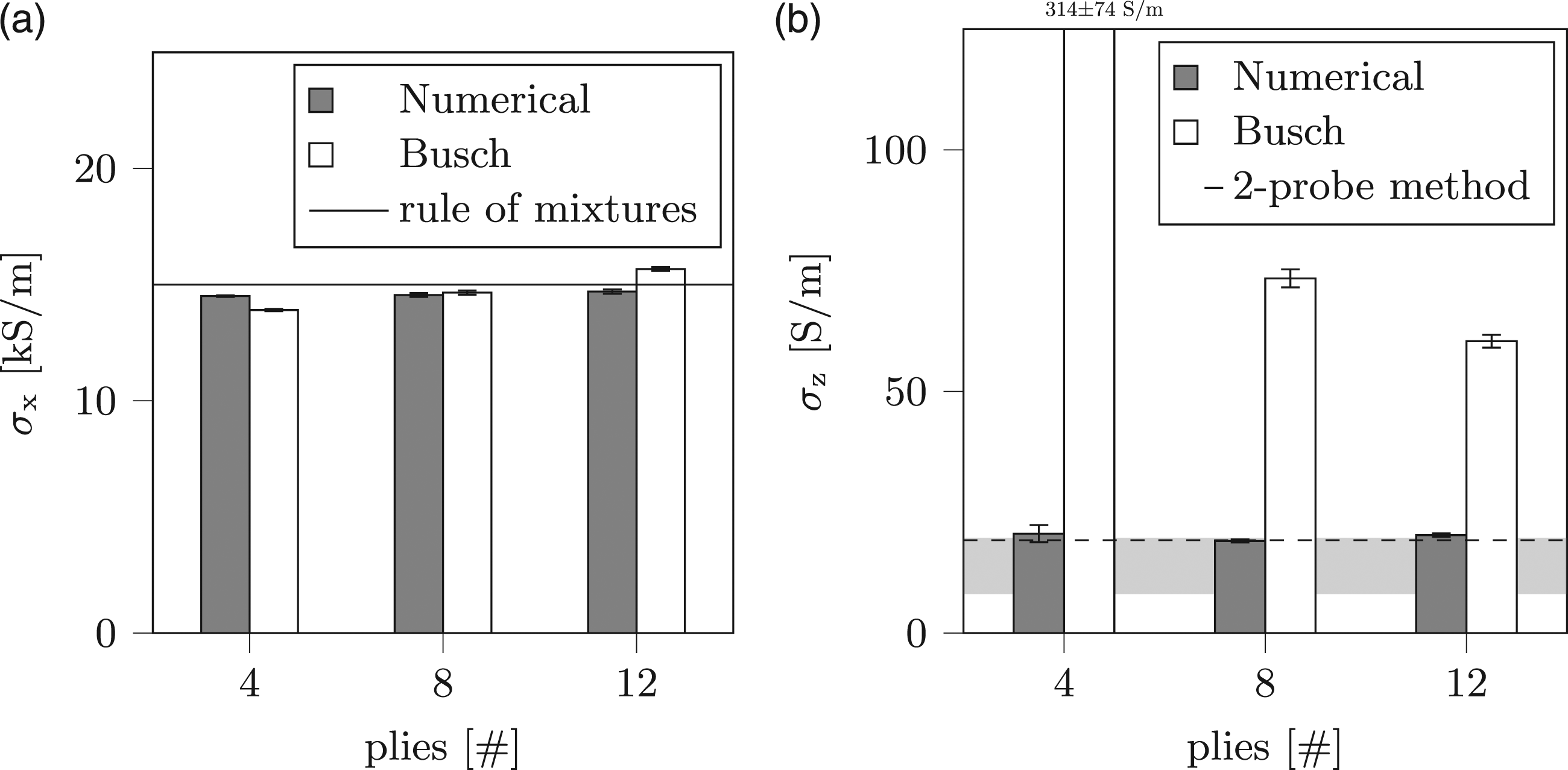
As mentioned in the above, the intercept of 62 ± 23 mΩ at t = 0 mm in Figure 14 represents the average contact resistance between electrode and specimen. This immediately emphasizes two limitations of the two-probe method. Firstly, contact resistance is difficult to avoid, even after a meticulous surface pretreatment as described in section. Secondly, to obtain an estimate of the contact resistance it is inevitable to use multiple specimens with different thicknesses. Based on the two-probe measurements on three different laminate thicknesses, only one average σz value was derived while the six-probe method does not require experiments on specimens with multiple thicknesses to characterise the anisotropic electrical conductivities.
A distinct difference in the σz values can be seen in Figure 11(b) compared to the σz values shown in Figure 15(b). In contrast to the σz values obtained in set A, shown in Figure 11(b), the σz values in Figure 15(b) does not show different σz values for the different specimen thicknesses. The obtained σz values in set D and E agree well with confidentially obtained σz values obtained from experiments on a large proprietary dataset which is shown by the gray area in the background of Figure 15(b). The limited amount of data in the present study is insufficient to make solid statements regarding thickness related phenomena affecting the out-of-plane electrical conductivity.
Conclusions
The overall objective of this study was to develop a simple and reliable method to measure the anisotropic electrical conductivity of a TPC material with a woven reinforcement. In this study, six-probe measurements were combined with a numerical approach to determine the anisotropic electrical conductivities. The study: • demonstrates that a 2-dimensional representation of the electrical current distribution in the six-probe method is justified, • shows that the present numerical method accurately calculates anisotropic electrical conductivities from six-probe measurements, • validates the in-plane electrical conductivities obtained by six-probe measurements with in-plane electrical conductivities obtained by rule of mixtures, • validates the out-of-plane electrical conductivities obtained by six-probe measurements with out-of-plane electrical conductivities obtained by two-probe measurements.
The conducted research shows that with one experiment, reliable in- and out-of-plane electrical conductivities of polymer composites reinforced with carbon fabrics can be determined simultaneously without the need of surface pretreatments. This represents an important simplification compared to other methods where the anisotropic electrical conductivities are determined with separate experiments and laborious surface pretreatments, required to ensure a proper introduction of the electrical current. The method can be applied to obtain the anisotropic electrical conductivity values required in induction heating simulations; another application beyond this paper is, for example, quality control of supplied materials.
Footnotes
Acknowledgements
The authors gratefully acknowledge the support from the industrial and academic members of the ThermoPlastic composites Research Center (TPRC), specifically the contribution from Toray Advanced Composites regarding the proprietary dataset on the σz values and the work done by TPRC students S. Barts and N. Pizzigoni are greatly appreciated.
Declaration of conflicting interests
The author(s) declared no potential conflicts of interest with respect to the research, authorship, and/or publication of this article.
Funding
The author(s) disclosed receipt of the following financial support for the research, authorship, and/or publication of this article: This work was supported by the industrial and academic members of the TPRC.
Appendix
Six-probe test results belonging to set A to investigate the influence of w and t on σ: I = 200 ± 5 mA, l = 40 mm, L = 120 mm.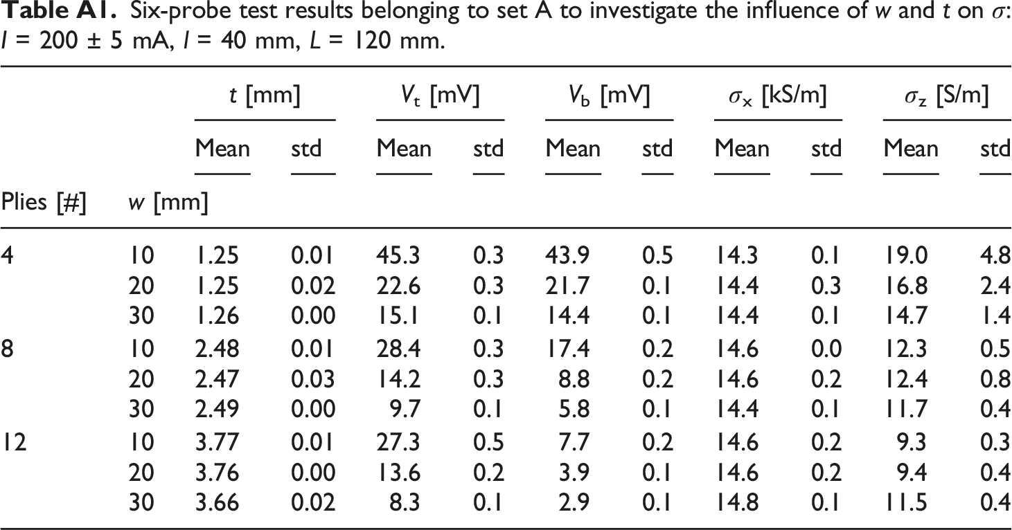
t [mm]
Vt [mV]
Vb [mV]
σx [kS/m]
σz [S/m]
Mean
std
Mean
std
Mean
std
Mean
std
Mean
std
Plies [#]
w [mm]
4
10
1.25
0.01
45.3
0.3
43.9
0.5
14.3
0.1
19.0
4.8
20
1.25
0.02
22.6
0.3
21.7
0.1
14.4
0.3
16.8
2.4
30
1.26
0.00
15.1
0.1
14.4
0.1
14.4
0.1
14.7
1.4
8
10
2.48
0.01
28.4
0.3
17.4
0.2
14.6
0.0
12.3
0.5
20
2.47
0.03
14.2
0.3
8.8
0.2
14.6
0.2
12.4
0.8
30
2.49
0.00
9.7
0.1
5.8
0.1
14.4
0.1
11.7
0.4
12
10
3.77
0.01
27.3
0.5
7.7
0.2
14.6
0.2
9.3
0.3
20
3.76
0.00
13.6
0.2
3.9
0.1
14.6
0.2
9.4
0.4
30
3.66
0.02
8.3
0.1
2.9
0.1
14.8
0.1
11.5
0.4
Six-probe test results belonging to set B to investigate the influence of l and L on σ with constant l/L-ratio: I = 200 ± 5 mA, w = 20 mm, l/L = 1/3.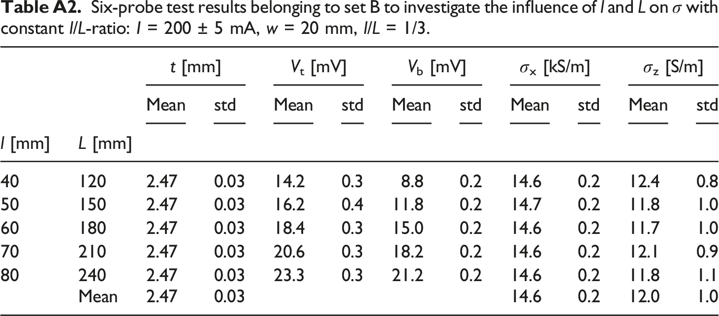
t [mm]
Vt [mV]
Vb [mV]
σx [kS/m]
σz [S/m]
Mean
std
Mean
std
Mean
std
Mean
std
Mean
std
l [mm]
L [mm]
40
120
2.47
0.03
14.2
0.3
8.8
0.2
14.6
0.2
12.4
0.8
50
150
2.47
0.03
16.2
0.4
11.8
0.2
14.7
0.2
11.8
1.0
60
180
2.47
0.03
18.4
0.3
15.0
0.2
14.6
0.2
11.7
1.0
70
210
2.47
0.03
20.6
0.3
18.2
0.2
14.6
0.2
12.1
0.9
80
240
2.47
0.03
23.3
0.3
21.2
0.2
14.6
0.2
11.8
1.1
Mean
2.47
0.03
14.6
0.2
12.0
1.0
Six-probe test results belonging to set C to investigate the influence of l and L on σ with varying l/L-ratio on the electrical conductivity is investigated: I = 200 ± 5 mA, w = 20 mm.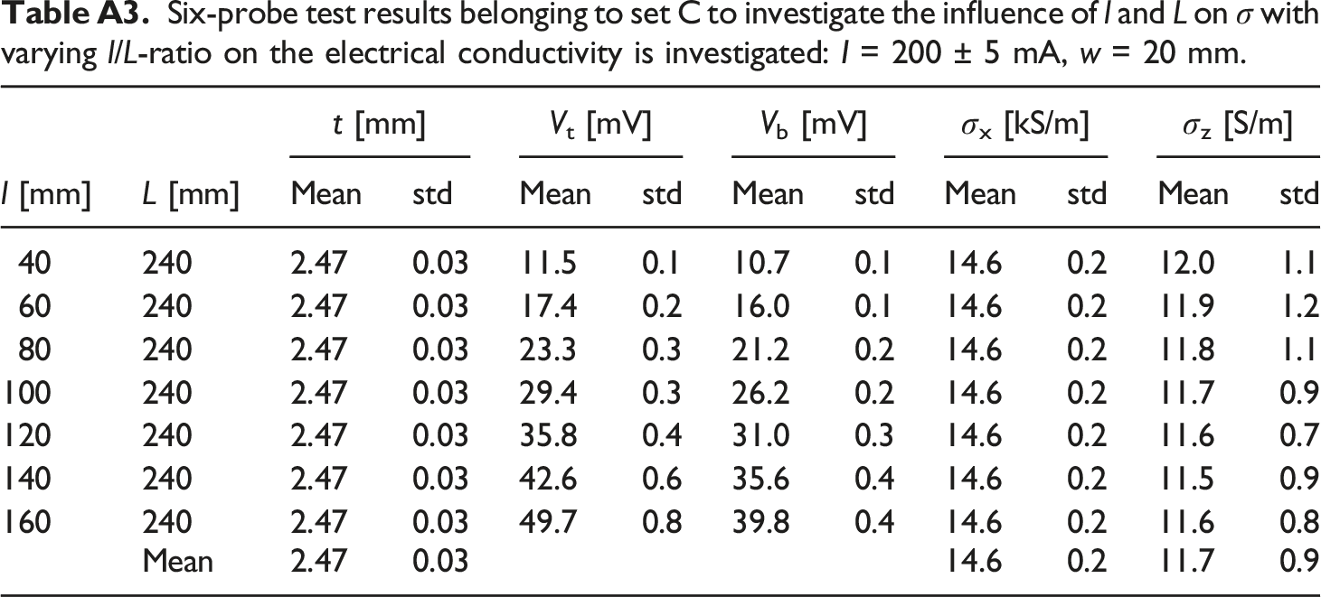
t [mm]
Vt [mV]
Vb [mV]
σx [kS/m]
σz [S/m]
l [mm]
L [mm]
Mean
std
Mean
std
Mean
std
Mean
std
Mean
std
40
240
2.47
0.03
11.5
0.1
10.7
0.1
14.6
0.2
12.0
1.1
60
240
2.47
0.03
17.4
0.2
16.0
0.1
14.6
0.2
11.9
1.2
80
240
2.47
0.03
23.3
0.3
21.2
0.2
14.6
0.2
11.8
1.1
100
240
2.47
0.03
29.4
0.3
26.2
0.2
14.6
0.2
11.7
0.9
120
240
2.47
0.03
35.8
0.4
31.0
0.3
14.6
0.2
11.6
0.7
140
240
2.47
0.03
42.6
0.6
35.6
0.4
14.6
0.2
11.5
0.9
160
240
2.47
0.03
49.7
0.8
39.8
0.4
14.6
0.2
11.6
0.8
Mean
2.47
0.03
14.6
0.2
11.7
0.9
Six-probe test results belonging to set D to validate the numerical method: I = 200 ± 5 mA, w = 20 mm, l = 40 mm, L = 120 mm.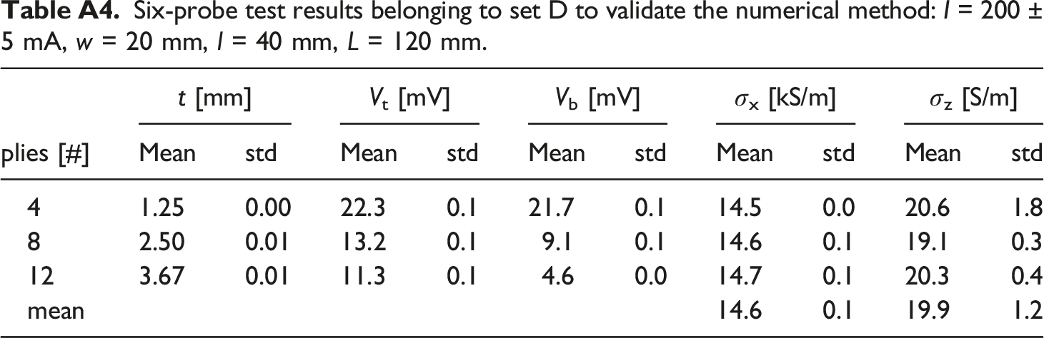
plies [#]
t [mm]
Vt [mV]
Vb [mV]
σx [kS/m]
σz [S/m]
Mean
std
Mean
std
Mean
std
Mean
std
Mean
std
4
1.25
0.00
22.3
0.1
21.7
0.1
14.5
0.0
20.6
1.8
8
2.50
0.01
13.2
0.1
9.1
0.1
14.6
0.1
19.1
0.3
12
3.67
0.01
11.3
0.1
4.6
0.0
14.7
0.1
20.3
0.4
mean
14.6
0.1
19.9
1.2
Two-probe test results belonging to set E to obtain σz-values to validate the numerical method with: I = 150 ± 5 mA, w × l = 15 × 15 mm.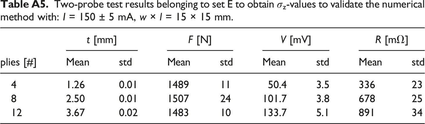
plies [#]
t [mm]
F [N]
V [mV]
R [mΩ]
Mean
std
Mean
std
Mean
std
Mean
std
4
1.26
0.01
1489
11
50.4
3.5
336
23
8
2.50
0.01
1507
24
101.7
3.8
678
25
12
3.67
0.02
1483
10
133.7
5.1
891
34