
Abstract
In the present article, the polymer melt impregnation of textile fiber reinforcements in an injection molding process is explored theoretically and experimentally. Simplifying the numerical simulation of the thermoplastic melt flow behavior a specific mold with integrated single-glass fiber bundle was developed and used for experimental fill studies with thermoplastic melt. The polymer melt impregnation of the fiber bundle in the injection molding process is modeled and calculated with Complex Rheology Polymer Solver (CoRheoPol), a simulation tool developed at Fraunhofer Institut fŭr Techno- und Wirtschaftsmathematik by the present authors. Navier-Stokes and Navier-Stokes-Brinkman equations are used to describe the melt flow in a pure fluid region and porous media, considering the non-Newtonian flow behavior of thermoplastic melts. Experimental and numerical results are compared determining the filling fronts and fiber impregnation of the injection molded test samples. A clear relationship between the degree of impregnation, verified by magnified photomicrograph, and the position of flow front can be detected. A good correlation of simulated and experimental flow fronts against the degree of filling of the mold is observed too. The differences in macroscopic flow behavior between the cavity with and without an integrated fiber bundle with respect to the impregnation process can be simulated with high accuracy.
Introduction
Textile-reinforced polymer composites feature outstanding mechanical properties through the possibility of adjusting the textile structure on existing distribution offorces. However, missing technologies for fast and fully automated production of textile composites based on thermoset resins still limit the applications to fieldswithlow volume production like aerospace or sports engineering. Highly efficient technologies for mass production of fiber-reinforced composites are available with thermoplastic matrix systems like injection molding or press technology. Traditionally, textile-reinforced thermoplastic composites are melt processed by compression molding. While press technology is suitable for large and plain-shaped structures, injection molding technology offers complex formed and highly function-integrated parts in combination with short cycle times, high repeat accuracy, and relatively low material costs.
Due to the plastification process, fiber-reinforced injection molded parts arecharacterized by irregular orientated fibers and short fiber lengths, limiting the mechanical properties. Especially the impact toughness and damage tolerance can be improved by using longer or endless fibers in thermoplastic composite materials.1,2 This is a crucial fact of interest for crash-sensitive structures, whichare primarily needed in high-volume automobile production. 3 To combine good mechanical properties and in particular high impact strength with effective injection molding technology, long fibers or a textile reinforcement has to be placed in the mold cavity.
The integration of thermoplastic prepregs in injection molding process is technically mature but rare in use due to the high material costs. 4 By using ‘dry’ textile structures, the melt impregnation, which means the encapsulation of every single fiber by the molten polymer, has to be assured within the injection process, which is a critical fact due to the high viscosity of thermoplastic melts. Inside of thefiber bundles the flow gaps are only of a few micrometers in diameter so that high pressure gradients are necessary for shifting the flow front and filling the gaps with the melt. 5 Early freezing of the flow front, caused by the heat transfer from the polymer melt to the cold cavity walls and fibers, is also a problematic fact. Therefore, the simulation of flow and impregnation processes of single fiber bundles is of vital importance for the configuration of suitable textile structures for the melt impregnation. Moreover, it is necessary to know how the injection molding process can be adjusted to the changed flow behavior, in order to minimize the costly and time-consuming experimental trial and error.
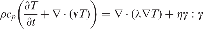
Considerable research efforts have been devoted to propose numerical modelsfor liquid composite molding (LCM) with thermoset resins, which mainly base on Darcy’s law. This empirical equation describes the flow of fluid through a porous media:
For polymer processes with high flow velocities, as occurring in injection molding processes, the general principles of fluid mechanics have to be applied and combined with the flow behavior in porous media, here the fiber bundles. Thenumerical simulation of the injection molding process of non-Newtonian fluids is a very challenging task. A system of thermal and incompressible Navier-Stokes equations with nonconstant viscosity has to be solved. The latter depends on shear rate, fluid temperature and can vary a couple of orders of magnitude within one simulation. It demands careful numerical treatment of the fluid stress tensor in momentum equations. 12 Viscosity is usually described by Carreau-type models, which account for shear thinning properties and strong exponential dependence on temperature. It is fitted to experimental curves by adjusting a set of model parameters. The bulk flow equations are solved in the presence of a freepropagating surface, which gives rise to additional complications. 13 Here, either interface-tracking or interface-capturing methods can be uses. 14 In the former, the surface is represented as a moving boundary, where the numerical grid moves with the surface. This method is usually used in computations of single-phase (one fluid) problems. In interface-capturing methods, the computational mesh is constructed once before the simulation starts. Then, the surface position is determined by computing fluid volume fraction (VOF) in each grid element. Such interface treatment allows the simulation of single-phase (fluids), as well as multiphase flow problems like two liquids or liquid–gas combinations. In this work, we use the VOF approach and consider a single-phase problem, that is, we do not simulate the flow of air, which is pushed away from the cavity by the entering polymer melt.
There are two ways to predict numerically the fiber impregnation in injection molding processes considered in this work. The geometry of the molded part with all details, including the structure of the fiber bundle, can be resolved. However, since the fiber diameter is of order of a few microns but the considered cavity of theorder of a few centimeters, the number of grid elements has to be enormously large. This would need an extensive amount of computational time and memory resources. Instead, fibers are treated as a macroscopic porous medium with effective model parameters, like permeability, upscaled from microscopic model and obtained empirically from experiments or derived from theory. 15 The advantage of the latter is that the grid number can be simultaneously kept in realistic bound and reflects the existence of fibers in the numerical algorithm. This leads to a system of Navier-Stokes equations for the pure fluid region and Navier-Stokes-Brinkman equations in the porous media, which are coupled to free surface flow and solved simultaneously.
Simulation background
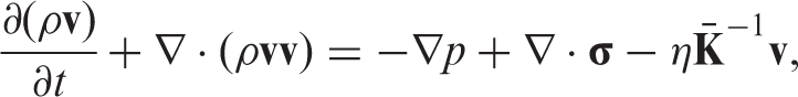
The Navier-Stokes-Brinkman macroscopic model has been successfully used in simulations of flow in porous media,
15
where a very good agreement with experimental measurements of pressure drop in oil flow through car filters has been achieved. The model consists of the incompressibility condition and the momentum balance:

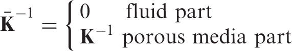
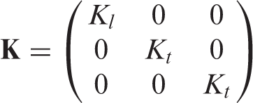
The permeability
In Laptev,
15
isothermal Newtonian flow has been considered. It fulfills a linear relation between the stress tensor and the velocity gradients with constant viscosity. However, physical processes are of interest, where non-Newtonian fluids withnonconstant viscosities have to be incorporated. The variations of the fluid viscosity are described with a Carreau-type
16
model:

Experimental
Processing method
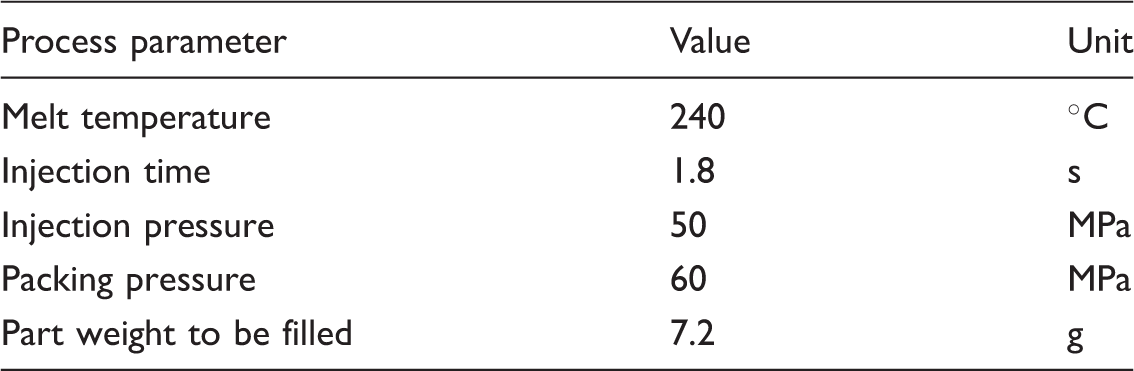
Process parameters of the injection molding test setup.
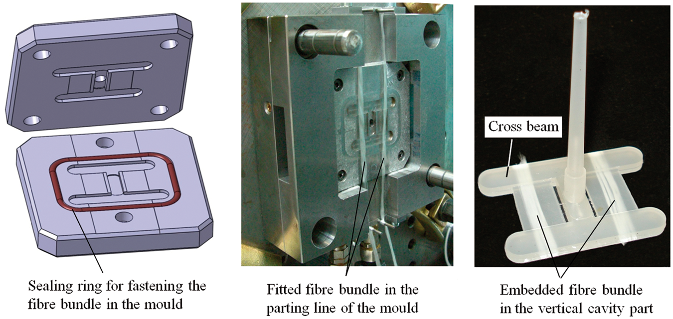
Injection mold (left and middle) and formed part with integrated fiber bundle (right).
Material parameters for simulation
Polypropylene homopolymer Moplen HP 500V, supplied by LyondellBasell, wasused for the melt impregnation of the fiber bundles. The high-fluidity polymer was measured with a melt flow rate (MFR) of 120 g/10 min (ISO 1133; 230°C/2.16 kg). The zero shear-rate viscosity was measured at 190°C with 220 Paċs and at 230°C with 85 Paċs. To consider the nonconstant melt viscosity in the simulation, it wasmeasured with rotational and capillary viscosimeter in the shear-rate range of 1 × 10⁻² and 2 × 10⁴/s, which typically occurs in injection molding processes. This was performed for melt temperatures of 190°C and 230°C to consider the dependency of temperature, too. Then, the flow curves were used to fit the Carreau-type model (Equation (6)). A distinctive shear thinning was measured, which results in a decrease of the viscosity below 10 Paċs (Figure 2). The needed values for the thermal conductivity and specific heat of the thermoplastic melt weretaken from the material database, supplied by the manufacturer. Thevalues were measured at 240°C melt temperature with a thermal conductivity of λ = 0.16 W/(mċK) and a specific heat of cp = 3010 J/(kgċK).
Flow curves for PP as measured and fit to Carreau-type model for simulation.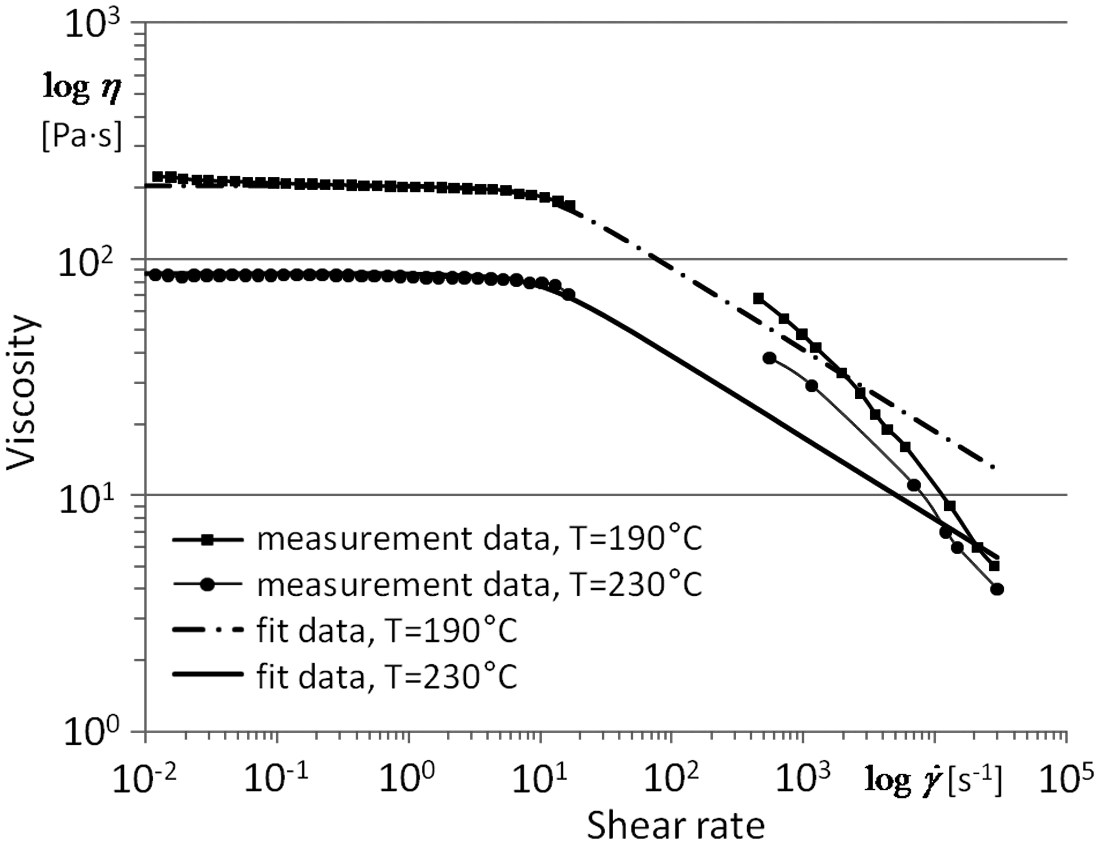
For the textile reinforcement, the commercially available E-glass direct rovingPR 440 2400 473A, supplied by Johns Manville, with 2400 tex was used, which corresponds approximately to 4100 single-fiber filaments. The fiber diameter was 17 µm. A silane/silicone sizing with concentration between 0.4 and 0.64 %w/w was determined by infrared (IR)-spectroscopy and thermogravimetric analysis. Theporosity was measured after impregnation tests, examining the polished specimen of photomicrographs, which were taken from the cross section of the roving. Several impregnated sections of some fiber bundles were examined and thefraction of glass fiber area within the area of enclosed fiber roving determined. An average value for the porosity of 0.2 was calculated. For converting the porosity in a permeability value, some theoretic formulas are available, which differ in respect to the applied models of fiber alignment or considering of capillary effects and imperfections in fiber packaging. 21 According to typical terms in literature, which were similar to the measured porosity value, permeability was set in the direction of fibers to 10–8/m2, 22 as in the perpendicular direction to 10–12/m2. 23
Filling study
For the comparison of numerical and experimental results, a filling study was carried out, which allowed to observe the tracking of the flow front in the mold. Therefore, the mold was filled partly with increasing filling degree, which was realized through a volume controlled injection, which stopped at defined positions of the plasticating screw. This was done for the mold with and without the fiber bundle to observe the differences in the flow process. Polished photomicrographs were made from the cross section of the embedded fiber bundles to observe the correlation of the flow front shifting and the level of impregnation.
Results
In this section, the simulation results will be presented. First, a two-dimensional (2D) example is used to validate the solver, where an isotropic permeability tensor is considered. Later, three-dimensional (3D) simulation results of the described injection molding process are shown and compared with experimental observations.
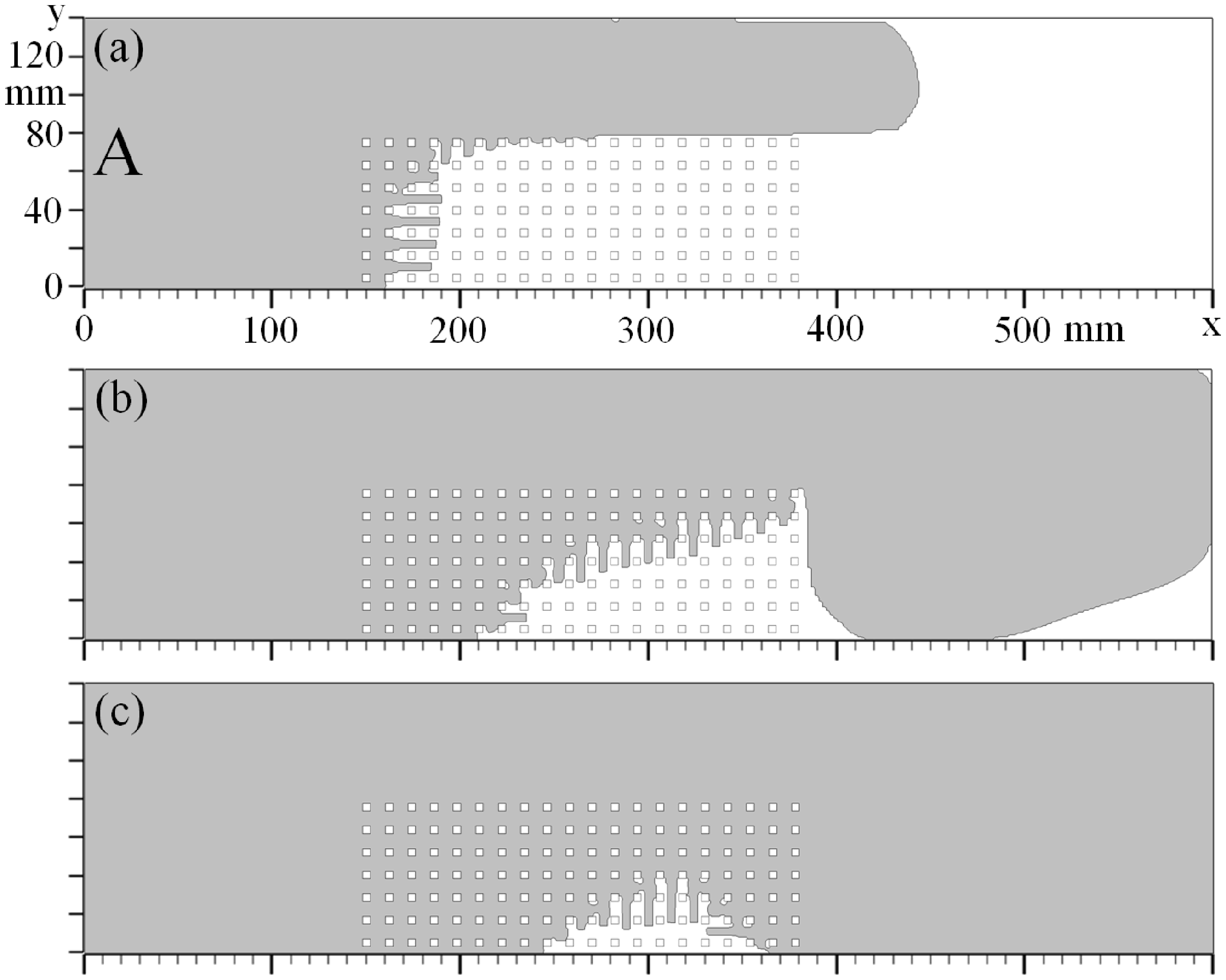
Flow through porous media in 2D channel
In a 2D test case, the performance of injection molding algorithms in a geometry with a porous part present was checked. A simulation was performed, where the porosity was either resolved geometrically, which we refer to micro case, or passed to the solver through the permeability tensor Validation of algorithm with porous part: Fluid fronts in three different stages of filling with porous media described through permeability tensor Validation of algorithm with porous part: Fluid fronts in three different stages of filling with geometrically resolved porosity.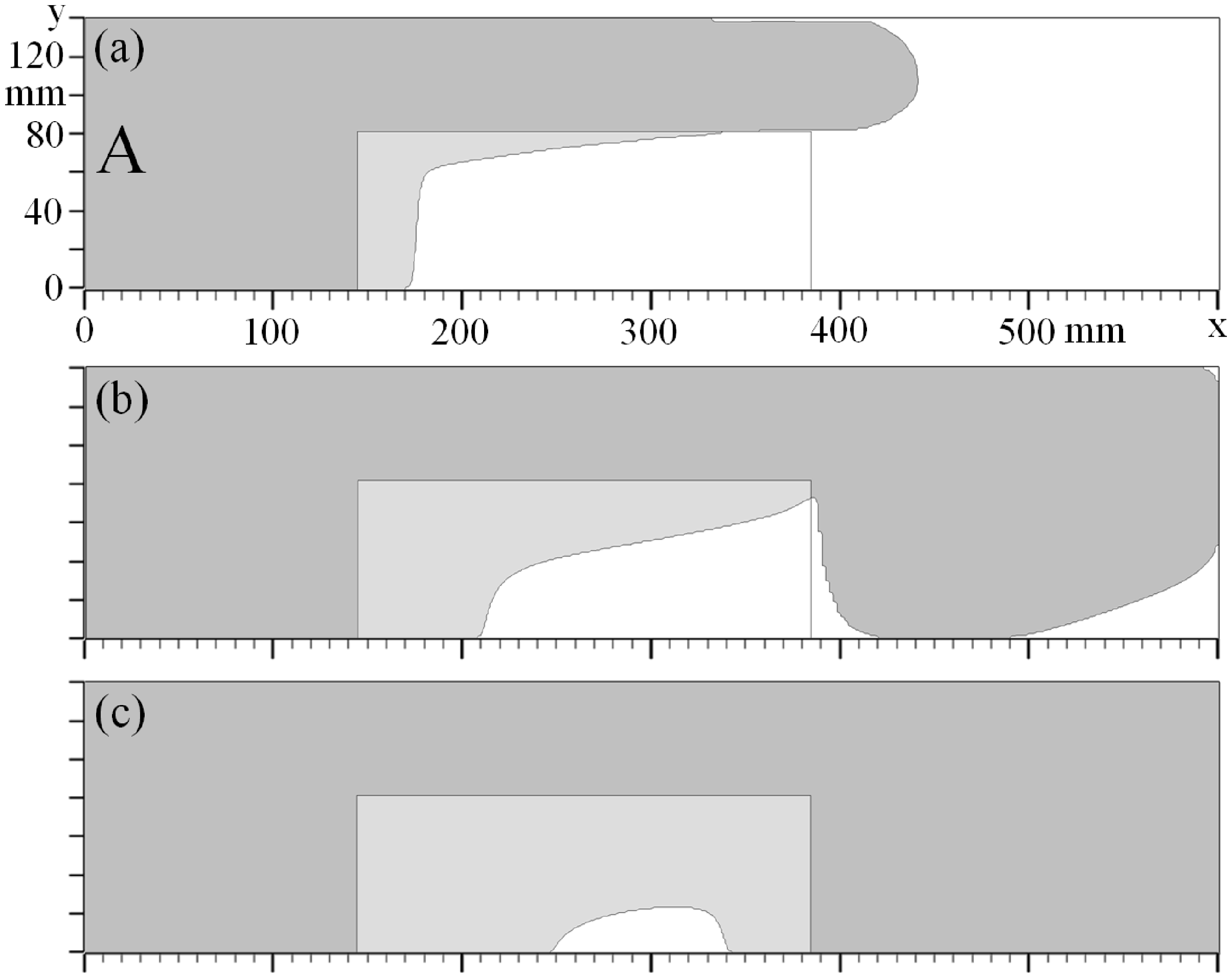
Filling of 3D mold
In the remaining subsection, comparisons of injection molding simulations with experimental observations will be presented. As shown in Figure 1 (right), the computer-aided design (CAD) model of the formed part was used to generate the computational grid with indicated porous part, that is, the region with fiber bundle. The lower cavity part (runner channel is not accounted) has dimensions of 60 × 40 × 4 mm, while the size of the fiber bundles is 5 × 40 × 0.25 mm. Following experimental measurements of the shearrate and the temperature depending viscosity (Figure 2) and fitting to Equation (6) the following fluid viscosity equation was used in simulations:

The thermal conductivity, specific heat, and permeability values were considered as described in section ‘Experimental.’ As indicated in Table 1, the whole filling process took about 1.8 s.
In order to perform systematic studies of our simulation algorithms, validation tests with injecting the polymer melt into the cavity without a fiber bundle were started. Parallel to the simulation, a series of experimental fill studies has been carried out. The injection process was stopped after filling consecutively increased volume fraction of the cavity. This allowed the comparison of fill fronts at the corresponding fill levels. When entering the cavity the fluid flows vertically along central part, reaches the cross beams of the double-T and starts to spread in horizontal directions (Figure 5(a)). As soon as the fluid attains the two vertical cavity parts, in this case without rovings, it begins to flow in vertical direction through the whole width of those geometry parts. Finally, the fluid fronts meet approximately in the middle vertical position. The front shapes are almost flat and spanned horizontally. A good correlation of the filling fronts in the simulation and experiment was observed. In Figure 5(a), a line A–B is indicated which marks the position of the flow velocity plot in Figure 5(b). The measurement points were taken from the middle plane of the cavity cross section. The cavity there is of dimension 14 × 2 mm. The magnitude of the melt flow velocity is given for the complete width of the cavity. The flow velocity plot shows an average magnitude of about 2.2 cm/s with a maximum of 2.5 cm/s outside of the centre line of the flow channel. In the near of the cavity walls a drastic slow-down can be observed as at the walls the velocity is zero by definition. The shift of the flow velocity maximum to the cavity wall, indicated with letter B, comes from the fact, that the fluid still didnot fully fill upper horizontal cavity part of the cross beam.
Melt flow behavior in the cavity without roving; (a) compare of the fluid fronts in the simulation (above) and experiment (below), (b) flow velocity in the cross section of the vertical cavity part.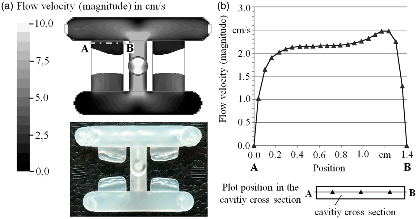
The next validation step was to compare the injection process with integrated fiber bundles in the two vertical cavity parts. All process conditions, like mold and fluid temperature, filling time, and more were the same as in the previously discussed attempts and specified in Table 1. In Figure 6(a), the comparison of the simulated and experimental filling study with integrated fiber bundles is shown. The injection process was stopped, when reaching the same injected melt volume as in the study before. The flow fronts reached an advanced fill level due to the integrated fiber bundles and therefore smaller ‘free’ cavity volume. In general, agood agreement of the flow behavior in the simulation and experiment could be observed. Variations results from the flexibility of the fiber bundle, which was not considered in the simulation. Caused by the flow pressure, a displacement of the fibers in the region of vertical melt overflow in the cross beams was observed. Thisleads to an unsymmetrical position of the fiber bundle in the vertical cavity parts. Therefore, the differences of the flow front position aside the roving are more distinctive between simulation and experiment.
Melt flow behavior in the cavity with integrated roving; (a) compare of the fluid fronts in the simulation (above) and experiment (below), (b) flow velocity in the cross section of the vertical cavity part.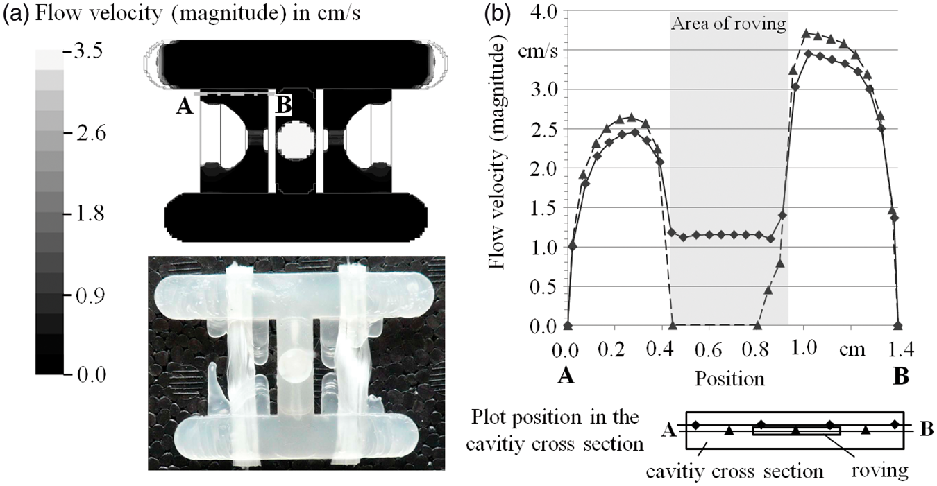
In Figure 6(a) also the line A–B is indicated which marks the position of the flowvelocity plots in Figure 6(b). The irregularities in the flow front along the roving are considerable more distinctive than in the flow study without roving, which results from the drastic slow-down of the flow velocity inside of the roving and also above and below it. The flow velocity curve along the line A–B through the roving in Figure 6(b) shows a maximum of 2.6 cm/s to the left and 3.7 cm/s tothe right of the roving but nearly a value of zero (0.01 cm/s) inside it. Also in the area just above the roving the flow velocity shows a slow-down to 1.2 cm/s which isless than the half of the flow velocity besides the roving. These decrease of the flow velocity results from the increasing flow resistance because of smaller available flow area. While above and beneath the roving the thickness of the flow channel is about half of the cavity thickness besides the roving, inside the flow gaps are of orders of magnitude smaller. The calculated flow velocities correspond to this. Incontrast, the maxima of flow velocity are higher as in the case without roving because of the same injection rate and lower ‘free’ cavity volume, that is, the volume not occupied by fiber bundle. The slow-down of the flow velocity above the fiber bundle is also the reason for the difference in flow velocity to the left and to the right of it. For filling the cavity part left to the roving (cavity side, indicated with the letter A in Figure 6(a)), it has to be partly overflowed in the cross beam, which leads to the described slow-down of flow velocity. This can be seen in the differences of the flow front positions in the filling study. On the side of the vertical cavity parts which are indicated with the letter B in Figure 6(a) the flow fronts are nearly in contact, on the other side they are still divided.
The drastic slow-down of the flow velocity along the flow gaps in the fiber bundle leads to a faster flow front tracking outside the roving. Therefore, the fiber bundle melt impregnation does not occurs in direction of the fibers butstarts with the melt overflow and is then almost perpendicularly adjusted to the fibers and overflow direction. For better understanding of this effect the examination of the polymer melt pressure along the flow path is necessary, as this is the driving force for the filling of the cavity and also for the impregnation of the fiber bundle. In Figure 7(a), the longitudinal section of the vertical cavity part with integrated fiber bundle is shown in the phase of 95% filling of the cavity. The plot thereby presents the melt pressure outside of the fiber bundle, the area inside is not taken into account. At the flow front the pressure is 0 and corresponds to the atmospheric pressure. Along the flow path a small increase up to 0.25 MPa can be detected, which results from the flow resistance of the viscous melt. Thepressure increase acts in all directions and starts to press the melt also into the fiber bundle. This process is schematically shown in Figure 7(b). Due to the increase of the pressure gradient along the flow path and corresponding speed up ofthe melt flow, differences of the impregnation level occur, which lead to a poor impregnation quality in fiber bundle segments at the end of the flow path. This is a crucial fact, since a faster flow front tracking outside the roving causes additionally an encapsulation of the air in the fiber bundle. In the packing phase, when the cavity is volumetrically filled, the pressure abruptly rises and pressurizes the melt. In our filling study a packing pressure of 60 MPa was adjusted (Table 1). Thus the melt impregnation level of the fiber bundle can be considerable improved by compression of the encapsulated air bubbles. However, they cannot disappear anymore and remain as voids in the fiber composite.
Melt pressure buildup along the flow path in the cavity; (a) melt pressure in the longitudinal section of the vertical cavity part, (b) schematic drawing of the fiber bundle impregnation as a function of the melt pressure.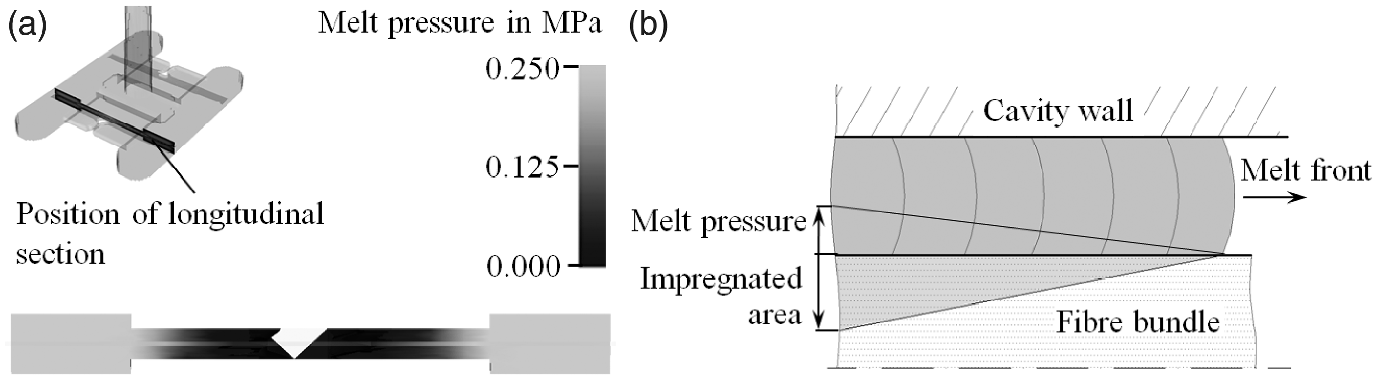
In the performed simulation and also in the experimental filling study the described process of fiber bundle impregnation could be determined. Figure 8(a) again shows the longitudinal section of the vertical cavity part with integrated fiber bundle, now in the moment of filling phase, when the flow fronts just contact in themiddle of the vertical cavity part. The cavity is nearly completely filled and the injection process will switch to packing phase. The simulation plot shows the flow velocity in the vertical cavity part. With a maximum flow velocity of 10 cm/s and a thickness of the flow channel of 1 mm above and beneath the fiber bundle, the shearrate is in the range of 101–102/s. Referring to the measured flow curve in Figure 2, the viscosity is only a little smaller compared to the zero shear rate viscosity. Thus, the positive shear thinning effect for the flowability of the high-viscous polymer melt can be neglected and has no influence on the impregnation process. In the simulation plot in Figure 8(a), the unfilled parts in the middle plane of the cavity, which correspond to the unimpregnated areas in the fiber bundle, can be clearly seen. In the contact zone of the two flow fronts, indicated with ‘2,’ the fiber bundle impregnation is very poor. With major distance of the flow front theimpregnation gets better, in the area of the cross beam, indicated with ‘1,’ already a full impregnation can be observed. For the compare of the simulated impregnation with the experimental filling study, polished photomicrographs were made from the cross section of the embedded fiber bundles. In Figure 8(b), exemplary photomicrographs are shown whose numbering corresponds to the indicated numbering in Figure 8(a) and describes the position in the fiber bundle. At the flow front (photomicrograph no. 2) the impregnation is very poor, only a few fiber layers are embedded in the polypropylene matrix. In the cross beam of the part (photomicrograph no. 1) the impregnation is much better. However, a complete impregnation, as calculated in the simulation, cannot be observed. Asdescribed, a single-phase problem was considered in the simulation and therefore the flow of the air, which is encapsulated in the embedded fiber bundle, was not taken into account. Apart from that the gradient of impregnation could be simulated very well and shows good correlation with the experiment.
Compare of the fiber bundle melt impregnation in the simulation and experiment; (a) simulation results of the melt flow velocity in the longitudinal section of the vertical cavity part, (b) photomicrographs of cross sections of an embedded fiber bundle at different positions along the flow path.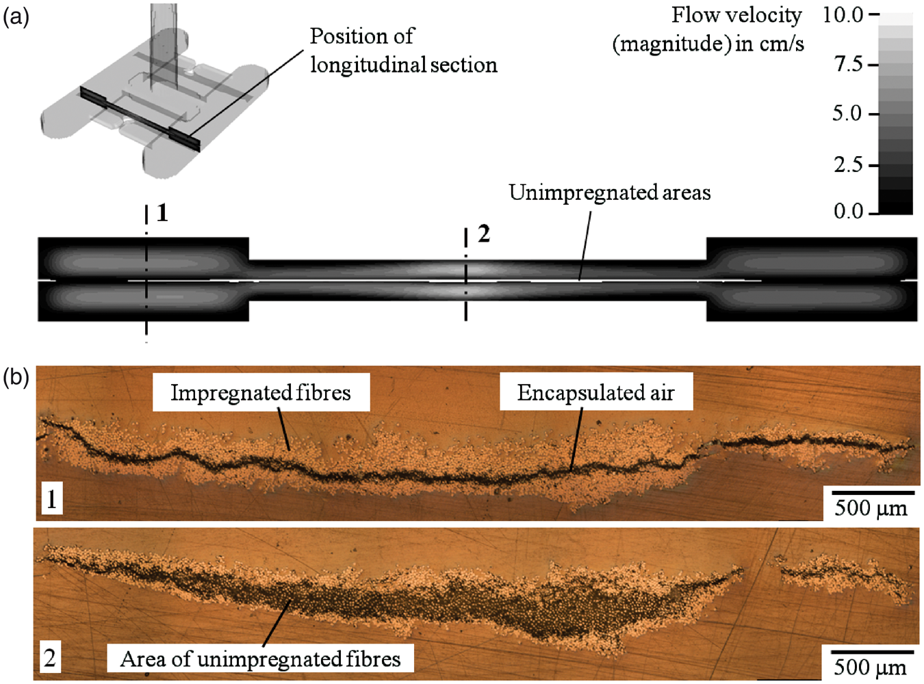
Conclusion
In the current work, we have presented a numerical approach to simulate injection molding processes for problems, where considered geometry posses both free fluid and porous parts simultaneously. Navier-Stokes and Navier-Stokes-Brinkmann equations for macroscopic description of flow behavior in the cavity with and without porous textile media were used, respectively. Injection molding tests were performed with a single-glass fiber bundle, overflowed lengthwise with a polypropylene melt, to verify the theoretical model. A distinctive slow-down of the melt flow velocity from maximum 3.7 cm/s outside to nearly zero inside of the fiber bundle was observed, which leads to a faster flow front tracking outside. Therefore, the melt impregnation results from the melt overflow and is almost perpendicularly adjusted to the fibers and overflow direction. The melt pressure could be identified as the driving force for the melt impregnation, which increases along the flow path. Apressure increase of 0.25 MPa within a flow path of 20 mm length was observed. Due to the pressure gradient, differences of the impregnation level occur which leadto a poor impregnation quality especially in fiber bundle segments at the end of the flow path. The faster flow front tracking outside the roving leads to an encapsulation of air in the fiber bundle, what could be verified in both simulation and experiment. The fractional impregnated rovings show a boundary area with embedded fibers, while the inner fibers remain unimpregnated and therefore without reinforcement effect. Overall the performed simulation shows good correlation with the experimental filling study. Small differences in simulated and experimental results come from the absence of the air flow in the cavity and neglecting the deformation of the fiber bundle in the simulation. Contrary to the experiment, in the simulation setup the fiber bundles are fixed and do not move within the injection process. It is clear, that both mentioned effects influence the flow of fluid during injection. However, the simulation could predict the impregnation of fiber bundles and the fill fronts well for both setups, the empty cavity and the cavity with fibers.
Footnotes
Funding
This work was performed within the research project PAFATHERM (Partial Textile Reinforcement of Thermoplastic Injection Moulded Parts) and supported by the German Federal Ministry of Education and Research within the initiative INNOPROFILE [grant number 03IP508].