Sage Journals: Discover world-class research

Abstract

A recent meta-analysis found reciprocal prospective effects between self-esteem and some aspects of work experience, for example, job satisfaction, and the authors concluded that their findings were consistent with a causal model, where self-esteem affects, and is affected by, work experiences. However, the prospective effects were estimated while adjusting for a prior measure of the outcome variable, and it is known that such adjusted cross-lagged effects may be spurious due to a correlation between the predictor and residuals in the initial measurement of the outcome and regression to the mean. The present reanalyses of the same meta-analytic data found all prospective effects between self-esteem and work experiences to be spurious. It is important for researchers to be aware of the limitations of adjusted cross-lagged effects in order not to overinterpret findings.

Keywords

Introduction

Given that many individuals spend a large portion of their time working, it is important to understand what factors contribute to job satisfaction and success at work, both in terms of external work conditions and personality traits, and the relationship between them. In a recent meta-analysis, Krauss and Orth (2022) identified reciprocal prospective effects between self-esteem and various measures of work experience, for example, job satisfaction. Krauss and Orth concluded that their findings were consistent with a causal model, where self-esteem affects, and is affected by, work experiences.

However, Krauss and Orth (2022) estimated cross-lagged prospective effects between self-esteem and work experiences while adjusting for a prior measure of the outcome, and it is known that such effects may be spurious due to a correlation between the predictor and residuals in the initial measurement of the outcome and regression to the mean (Castro-Schilo & Grimm, 2018; Eriksson & Häggström, 2014; Glymour et al., 2005; Sorjonen et al., 2019).

Regression to the mean is a phenomenon where measured scores tend to change toward expected scores between measurements. This is expected to happen when the test-retest correlation of the variable is less than 1 (equation (1), where E|Z_Y2| = expected standardized score on Y at time 2, Z_Y1 = standardized score on Y at time 1, r_Y1,Y2 = test-retest correlation for the measurement of Y, (Cohen et al., 2003)). For example, imagine a population where mean Y-score equals 4 (SD = 1). From this population, we draw three individuals A, B, and C and their measured Y-score at time 1 equals 2, 4, and 6, respectively, which corresponds to standardized scores −2, 0, and 2. If we assume a test-retest correlation of .8 for the Y-score, the expected standardized scores at a subsequent measurement equals −1.6, 0, and 1.6 for the three individuals, respectively, (see equation (1)). Assuming the same mean and standard deviation at the two measurements (i.e., M = 4, SD = 1), these standardized scores correspond to the unstandardized scores 2.4, 4, and 5.6. Consequently, the expected change between the two measurements, the regression toward the mean, equals .4, 0, and −.4 for the three individuals, respectively (Figure 1).

E | Z_{Y 2} | = Z_{Y 1} \times r_{Y 1, Y 2}

(1)

Figure 1.

Predicted change in Y-score between time 1 and time 2 for three hypothetical individuals drawn from a hypothetical population with a mean Y-score equal to 4 (SD = 1) and a test-retest correlation in the measurement of the Y-score equal to .8.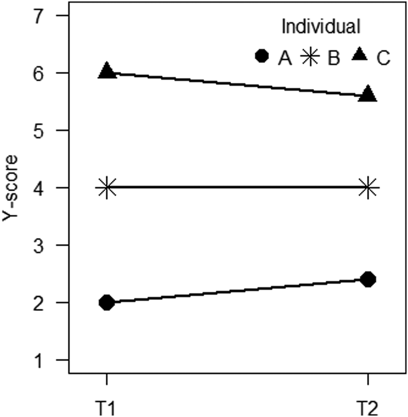

For a more elaborate example, we consider a predictor X in addition to the two measurements Y1 and Y2 (Table 1 and Figure 2). In this hypothetical situation, we have a positive association between X and Y on the population level, with the highest mean/expected value on Y (= 6) for those with the highest value on X (= 5) and the lowest mean/expected value on Y (= 2) for those with the lowest value on X (= 1) (column 2 in Table 1). We assume a standard deviation of .5 for the Y-score in all subpopulations with different X-scores, both at time 1 and at time 2. From this population, we draw a sample of 20 individuals (the rows in Table 1) and measure their Y-score at time 1 (column 3 in Table 1). Now we can standardize each individual’s Y-score within subpopulations (column 4 in Table 1). For example, individual 7 has a Y-score of 4.5 compared with an expected score of 6 (due to her/his X-score of 5) and, consequently, a Z-score of (4.5–6)/0.5 = −3. We assume a test-retest correlation of .8 between Y1 and Y2 (on the population level). Consequently, the expected standardized Y-score at time 2 is given by (see equation (1)) Z(Y1) × .8 (column 5 in Table 1). The expected standardized Y-score at time 2 can be transformed to an unstandardized expected Y-score (column 6 in Table 1). For example, for individual 7, the expected Y-score at time 2 equals −2.4 × .5 + 6 = 4.8. Expected change in the Y-score between time 1 and time 2 (column 7 in Table 1) equals the difference between expected Y-score at time 2 (column 6 in Table 1) and observed Y-score at time 1 (column 3 in Table 1). For example, for individual 7, expected change equals 4.8–4.5 = .3.

Table 1.

A Hypothetical Example with 20 Individuals With Different X-scores (Column 1) and, Consequently, Different Expected Y-scores (Column 2) and Change in the Y-score Between Time 1 and Time 2 (Columns 7 and 12). These Data are Illustrated in Figure 2 (Columns 3–7 in Panel A and Columns 8–12 in Panel B).

Ind.	Adj. for Y1 (Panel A)							Adj. for Y2 (Panel B)
Ind.	1.X	2.E\|Y\|	3.Y1	4.Z (Y1)	5.E\|Z (Y2)\|	6.E\|Y2\|	7.E\|Δ\|	8.Y2	9.Z (Y2)	10.E\|Z (Y1)\|	11.E\|Y1\|	12.E\|Δ\|
1	5	6	7.5	3	2.4	7.2	−0.3	7.5	3	2.4	7.2	0.3
2	5	6	6.5	1	0.8	6.4	−0.1	6.5	1	0.8	6.4	0.1
3	4	5	6.5	3	2.4	6.2	−0.3	6.5	3	2.4	6.2	0.3
4	5	6	5.5	−1	−0.8	5.6	0.1	5.5	−1	−0.8	5.6	−0.1
5	4	5	5.5	1	0.8	5.4	−0.1	5.5	1	0.8	5.4	0.1
6	3	4	5.5	3	2.4	5.2	−0.3	5.5	3	2.4	5.2	0.3
7	5	6	4.5	−3	−2.4	4.8	0.3	4.5	−3	−2.4	4.8	−0.3
8	4	5	4.5	−1	−0.8	4.6	0.1	4.5	−1	−0.8	4.6	−0.1
9	3	4	4.5	1	0.8	4.4	−0.1	4.5	1	0.8	4.4	0.1
10	2	3	4.5	3	2.4	4.2	−0.3	4.5	3	2.4	4.2	0.3
11	4	5	3.5	−3	−2.4	3.8	0.3	3.5	−3	−2.4	3.8	−0.3
12	3	4	3.5	−1	−0.8	3.6	0.1	3.5	−1	−0.8	3.6	−0.1
13	2	3	3.5	1	0.8	3.4	−0.1	3.5	1	0.8	3.4	0.1
14	1	2	3.5	3	2.4	3.2	−0.3	3.5	3	2.4	3.2	0.3
15	3	4	2.5	−3	−2.4	2.8	0.3	2.5	−3	−2.4	2.8	−0.3
16	2	3	2.5	−1	−0.8	2.6	0.1	2.5	−1	−0.8	2.6	−0.1
17	1	2	2.5	1	0.8	2.4	−0.1	2.5	1	0.8	2.4	0.1
18	2	3	1.5	−3	−2.4	1.8	0.3	1.5	−3	−2.4	1.8	−0.3
19	1	2	1.5	−1	−0.8	1.6	0.1	1.5	−1	−0.8	1.6	−0.1
20	1	2	0.5	−3	−2.4	0.8	0.3	0.5	−3	−2.4	0.8	−0.3

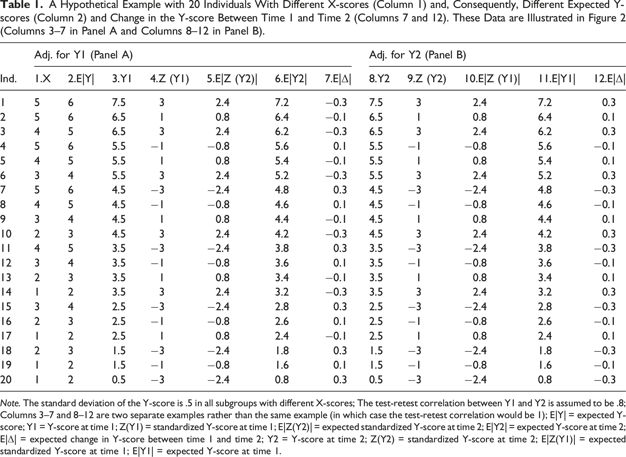
Note. The standard deviation of the Y-score is .5 in all subgroups with different X-scores; The test-retest correlation between Y1 and Y2 is assumed to be .8; Columns 3–7 and 8–12 are two separate examples rather than the same example (in which case the test-retest correlation would be 1); E|Y| = expected Y-score; Y1 = Y-score at time 1; Z(Y1) = standardized Y-score at time 1; E|Z(Y2)| = expected standardized Y-score at time 2; E|Y2| = expected Y-score at time 2; E|Δ| = expected change in Y-score between time 1 and time 2; Y2 = Y-score at time 2; Z(Y2) = standardized Y-score at time 2; E|Z(Y1)| = expected standardized Y-score at time 1; E|Y1| = expected Y-score at time 1.

Figure 2.

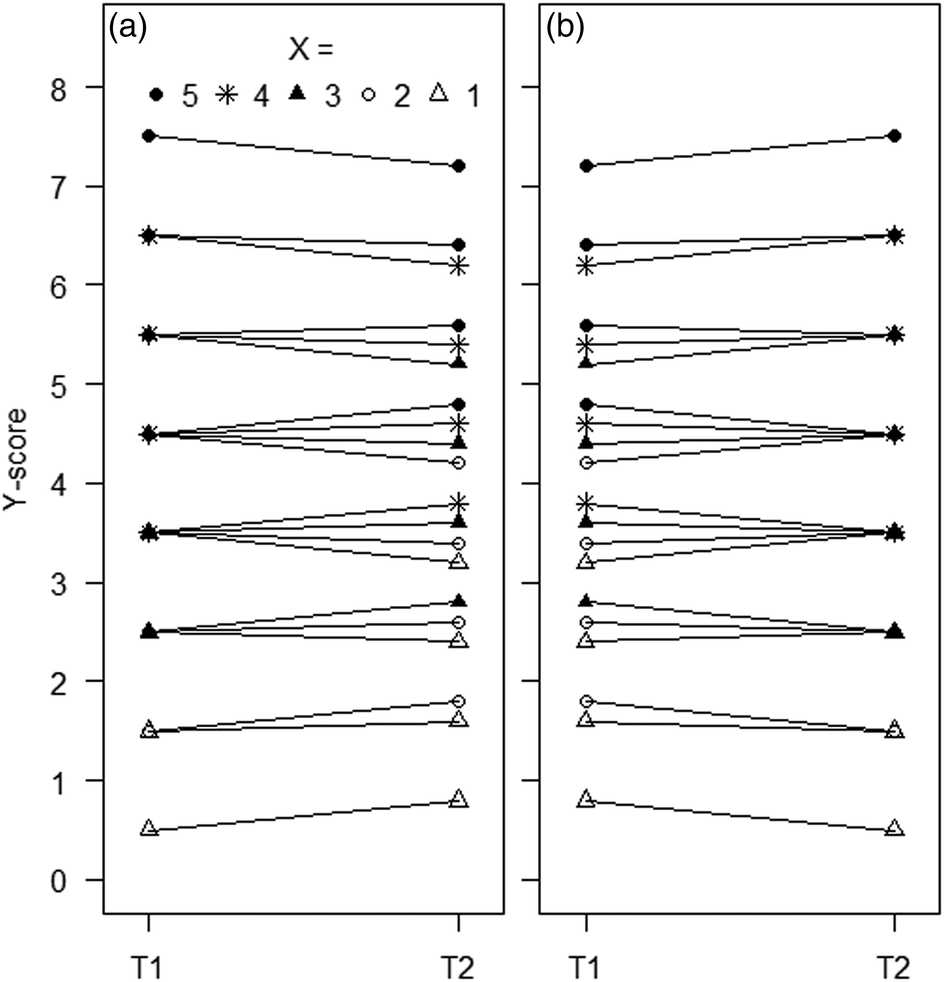
Values for the Figure comes from Table 1. The example assumes a positive association between X and Y. (a) For individuals with the same value on Y1, we expect a more positive, but spurious, change in Y between T1 and T2 for those with a high value on X compared with those with a lower value on X, even if no true change in Y has taken place. Consequently, we expect a positive, but spurious, effect of X on Y2 when adjusting for Y1. (b) For individuals with the same value on Y2, we expect those with a high value on X to have had a higher value on Y1 and, consequently, to have experienced a more negative change in Y between T1 and T2 compared with those with the same value on Y2 but with a lower value on X. This means that we expect to see a positive, but spurious, effect of X on Y1 when adjusting for Y2. Note: Panels A and B are two separate, but mirrored, examples rather than the same example (in which case the test-retest correlation of Y would be 1 and no regression to the mean would be expected).

These expected changes are illustrated in Figure 2, panel A. For each Y-score at time 1, those with a higher X-score are expected to experience a more positive change in the Y-score between time 1 and time 2 compared with those with a lower X-score. This means that we would see a positive effect of X on Y2 when adjusting for Y1. However, the effect is spurious rather than indicating a true increasing effect of X on Y. The effect is due to the fact that for a given observed Y-score at time 1, those with a higher X-score are further below their expected Y-score and can be assumed to have received a lower Y-score compared with their true Y-score, that is, a more negative residual, compared with those with the same Y1-score but a lower X-score. However, residuals tend to regress toward a mean value of zero between measurements and we can, consequently, expect a more positive, but spurious, change in the Y-score between time 1 and time 2 for those with a high X-score compared with those with the same Y-score at time 1 but with a lower X-score.

Such an effect of X on Y2 when adjusting for Y1 may be spurious, rather than due to a true increasing or decreasing effect, which can be made apparent by reversing the analysis and estimate the effect of X on Y1 when adjusting for Y2. In Table 1, we see that some individuals have a higher Y-score at time 2 (column 8) compared with their expected Y-score (column 2) and, consequently, a positive standardized Y-score at time 2 (column 9). Conversely, others have a lower Y2-score compared with their expected score and, consequently, a negative standardized Y2-score. As the test-retest correlation equals .8, individuals are expected to have had a 20% more attenuated standardized score at time 1 than at time 2 (column 10 in Table 1, see equation (1)). For those who are above their expected value on Y at time 2, this means that they are expected to have had a lower Y-score at time 1 (column 11 in Table 1) and, consequently, to have experienced an increase in the Y-score between time 1 and time 2 (column 12 in Table 1). Conversely, those who are below their expected Y-score at time 2 are expected to have had a higher Y-score at time 1 and, consequently, to have experienced a decrease in the Y-score between time 1 and time 2.

In summary, what this example shows is that with a positive association between X and Y and less than perfect reliability in the measurement of Y, we can expect a positive, but spurious, effect of X on Y2 when adjusting for Y1 (Figure 2, panel A) but also a positive effect of X on Y1 when adjusting for Y2 (Figure 2, panel B). However, while the former positive effect suggests an increasing effect of X on Y, the latter positive effect suggests a decreasing effect of X on Y. We think that if analysis of the same data would suggest simultaneous increasing and decreasing effects of X on Y that the effects should be ruled out as spurious.

For an example involving self-esteem and work experiences, let us assume a general positive association between self-esteem and job satisfaction. This positive association could, for example, be due to a confounding influence of a general positivity/negativity trait. Among individuals with the same initial measured job satisfaction but with different initial measured self-esteem, we can suspect a more negative residual in the measurement of job satisfaction among those with high self-esteem and a more positive residual among those with low self-esteem. However, as residuals tend to regress toward a mean value of zero between measurements, we can expect a positive, but spurious, effect of initial self-esteem on subsequent job satisfaction when adjusting for initial job satisfaction, even if no true change in job satisfaction has taken place. Furthermore, if the effect is spurious, we can also expect a positive effect of initial self-esteem on initial job satisfaction when adjusting for subsequent job satisfaction, even if this positive effect would suggest, paradoxically, a degrading prospective effect of self-esteem on job satisfaction.

The objective of the present study was to evaluate if the prospective associations between self-esteem and work experiences found by Krauss and Orth (2022) were truly increasing or decreasing, or spurious due to a correlation between the predictor and residuals in the initial measurement of the outcome and regression to the mean. See the method section for predictions. The overall aim of the meta-analytic reanalyses was to contribute with knowledge of the limitations of cross-lagged panel analyses, and highlight the importance of not over-interpreting findings.

Method

We refer to Krauss and Orth (2022) for more comprehensive information on selection of studies, test of publication bias, etc. In short, Krauss and Orth identified 31 longitudinal studies (of 30 independent samples, total N = 53,112, mean age at initial measurement = 36.7 years (SD = 11.4), mean proportion of female participants = 48% (SD = 25%)) with measures of self-esteem and at least one of the following aspects of work experience: (1) Employment status; (2) Income; (3) Job resources, for example, support from supervisor; (4) Job satisfaction; (5) Job stressors, for example, time pressure; (6) Job success, for example, occupational prestige. From the included studies, Krauss and Orth extracted: (a) the concurrent correlation between initial self-esteem and initial work experience; (b) autoregressive correlations between initial and subsequent self-esteem and work experience; and (c) cross-lagged correlations between initial self-esteem and subsequent work experience, and vice versa.

Krauss and Orth (2022) used equation (2) (Cohen et al., 2003) to estimate the standardized regression effect of initial self-esteem on subsequent work experience while adjusting for initial work experience, and vice versa. In addition to estimating the adjusted prospective effects between self-esteem and work experience, we used equation (2) to estimate the effect of initial self-esteem on initial work experience while adjusting for subsequent work experience, and vice versa. Furthermore, we used equation (3) (Guilford, 1965) to estimate the effect of initial self-esteem on subsequent change in work experience, and vice versa.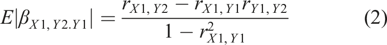

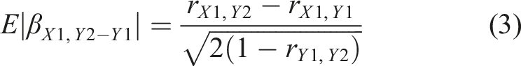
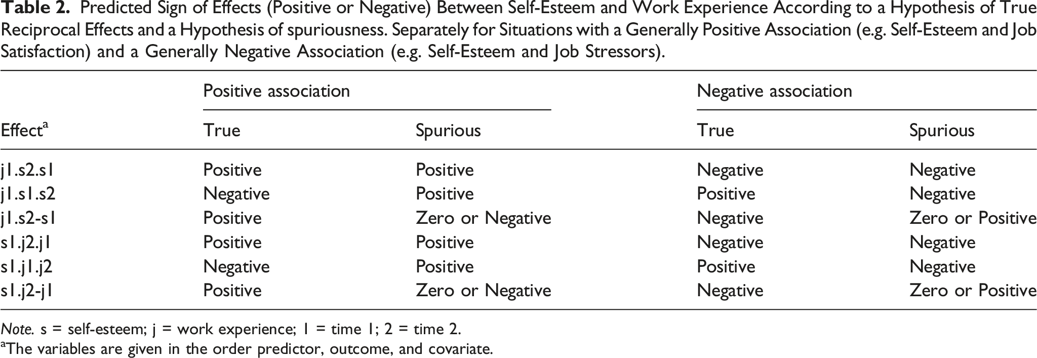
E | β_{X 1, Y 2 . Y 1} | = \frac{r_{X 1, Y 2} - r_{X 1, Y 1} r_{Y 1, Y 2}}{1 - r_{X 1, Y 1}^{2}}

(2)

E | β_{X 1, Y 2 - Y 1} | = \frac{r_{X 1, Y 2} - r_{X 1, Y 1}}{\sqrt{2 (1 - r_{Y 1, Y 2})}}

(3)

Table 2 summarizes predictions by a hypothesis of true increasing or decreasing prospective effects between self-esteem and work experiences and a hypothesis of spurious effects due to a correlation between the predictor and residuals in the initial measurement of the outcome and regression to the mean. Here, we exemplify with an effect of self-esteem on job satisfaction:

(1a) If self-esteem had a true increasing prospective effect on job satisfaction, we expect a positive effect of initial self-esteem on subsequent job satisfaction when adjusting for initial job satisfaction. For example, if a group with high initial self-esteem and a group with low initial self-esteem had the same average initial job satisfaction (e.g. 0), we would expect a higher average subsequent job satisfaction for those with high initial self-esteem (e.g. .5) compared with those with low initial self-esteem (e.g. −.5) as this would mean a more positive change in job satisfaction between measurements for those with high initial self-esteem (.5 – 0 = .5) compared with those with low initial self-esteem (−.5 – 0 = −.5).

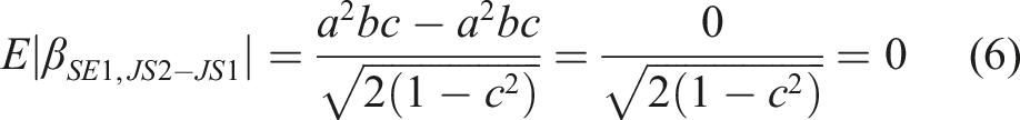
(1b) However, also a hypothesis of spuriousness predicted this effect to be positive. For example, if data was generated as in Figure 3, without any true prospective effects between self-esteem and job satisfaction, the expected correlation between SE₁ and JS₂ and between SE₁ and JS₁ equals b × a × a × c = a²bc, and the expected correlation between JS₁ and JS₂ equals c × c = c². If we plug these values into equation (2), we receive

E | β_{S E 1, J S 2 . J S 1} | = \frac{a^{2} b c - a^{2} b c ∙ c^{2}}{1 - {(a^{2} b c)}^{2}} = \frac{a^{2} b c (1 - c^{2})}{1 - {(a^{2} b c)}^{2}}

(4)

Table 2.

Predicted Sign of Effects (Positive or Negative) Between Self-Esteem and Work Experience According to a Hypothesis of True Reciprocal Effects and a Hypothesis of spuriousness. Separately for Situations with a Generally Positive Association (e.g. Self-Esteem and Job Satisfaction) and a Generally Negative Association (e.g. Self-Esteem and Job Stressors).

Effect^a	Positive association		Negative association
Effect^a	True	Spurious	True	Spurious
j1.s2.s1	Positive	Positive	Negative	Negative
j1.s1.s2	Negative	Positive	Positive	Negative
j1.s2-s1	Positive	Zero or Negative	Negative	Zero or Positive
s1.j2.j1	Positive	Positive	Negative	Negative
s1.j1.j2	Negative	Positive	Positive	Negative
s1.j2-j1	Positive	Zero or Negative	Negative	Zero or Positive

Note. s = self-esteem; j = work experience; 1 = time 1; 2 = time 2.

^aThe variables are given in the order predictor, outcome, and covariate.

Figure 3.

A hypothetical data generating model where general (i.e. trait-like) self-esteem (gSE) and job satisfaction (gJS) affect measurements at two separate occasions and are, in turn, affected by a common confounding factor (Conf.). Although the model does not include any true prospective effects between self-esteem and job satisfaction, we may still expect spurious effects of initial self-esteem on subsequent job satisfaction when adjusting for initial job satisfaction, and vice versa. See the text for a more comprehensive description.

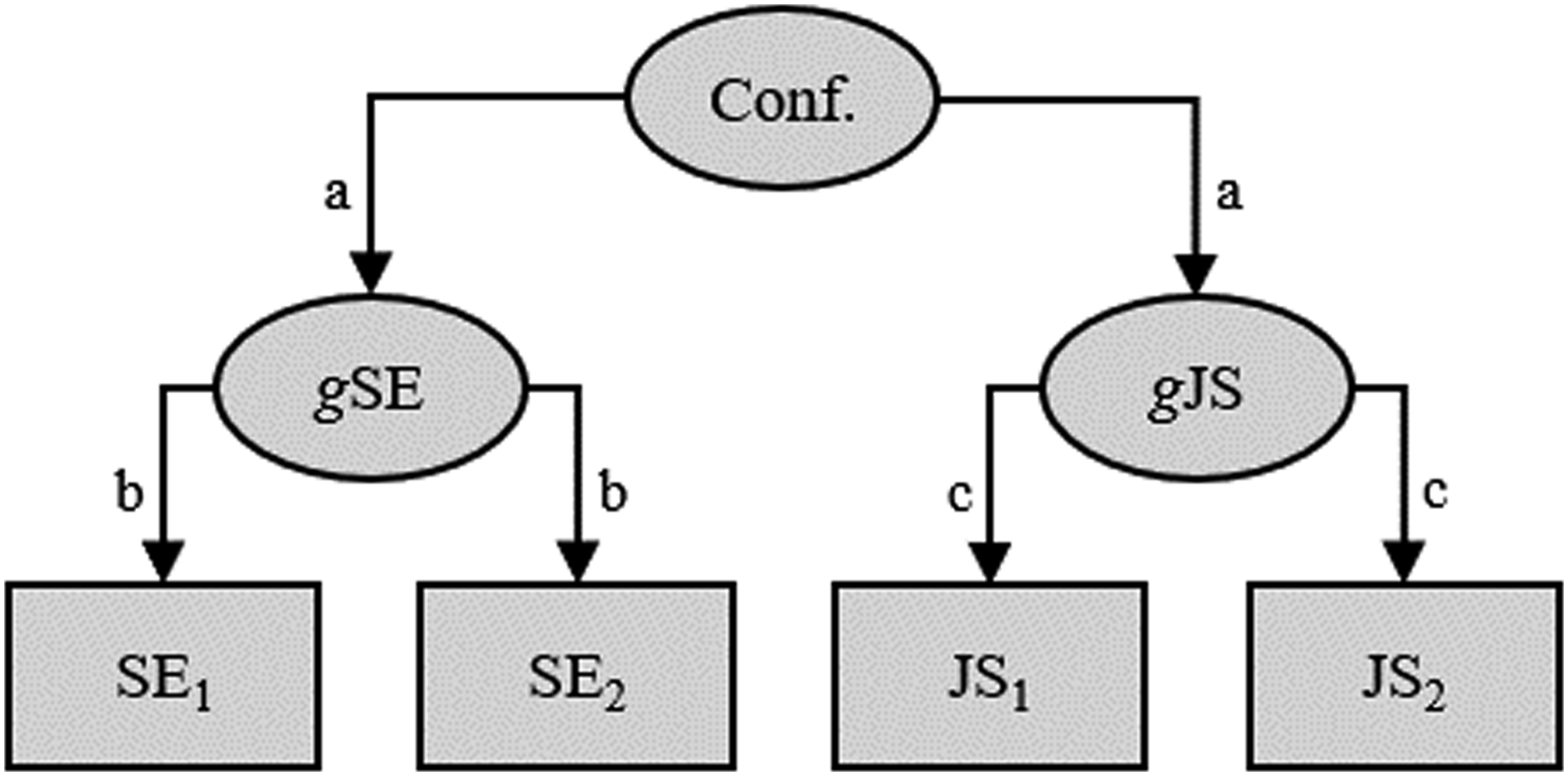
If we assume that all three standardized effects a, b, and c in Figure 3 were between (but did not include) 0 and 1, both the numerator and the denominator in equation (4) would also be between (but not include) 0 and 1, and the expected standardized effect of initial self-esteem on subsequent job satisfaction while adjusting for initial job satisfaction would be positive (>0), even if data was generated by a model with no true increasing prospective effect of self-esteem on job satisfaction. In Figure 3, the labelled parameters stand for: (a) the effect of a common confounder on general self-esteem and general job satisfaction; (b) the effect of general self-esteem on measured self-esteem at time 1 and time 2; and (c) the effect of general job satisfaction on measured job satisfaction at time 1 and time 2.

(2a) A hypothesis of a true increasing prospective effect predicted a negative effect of initial self-esteem on initial job satisfaction when adjusting for subsequent job satisfaction. This effect was predicted to be negative because among individuals with the same subsequent job satisfaction, the lower the initial job satisfaction, the larger the increase in job satisfaction between measurements. For example, if a group with high initial self-esteem and a group with low initial self-esteem had the same average subsequent job satisfaction (e.g. 0), we would expect a lower average initial job satisfaction for those with high initial self-esteem (e.g. −.5) compared with those with low initial self-esteem (e.g. .5) as this would mean a more positive change in job satisfaction between measurements for those with high initial self-esteem (0 – (−.5) = .5) compared with those with low initial self-esteem (0 – .5 = −.5).

(2b) Contrarily, a hypothesis of spuriousness predicted this effect to be positive. For example, if data is generated as in Figure 3, without any true prospective effects between self-esteem and job satisfaction, the expected standardized effect of initial self-esteem on initial job satisfaction while adjusting for subsequent job satisfaction (see above for expected correlations) equals

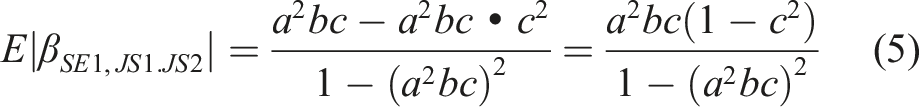
E | β_{S E 1, J S 1 . J S 2} | = \frac{a^{2} b c - a^{2} b c ∙ c^{2}}{1 - {(a^{2} b c)}^{2}} = \frac{a^{2} b c (1 - c^{2})}{1 - {(a^{2} b c)}^{2}}

(5)

Consequently, if data is generated as in Figure 3, without any true prospective effects between self-esteem and job satisfaction, the standardized effect of initial self-esteem on initial job satisfaction while adjusting for subsequent job satisfaction (equation (5)) is expected to be the same as the standardized effect of initial self-esteem on subsequent job satisfaction while adjusting for initial job satisfaction (equation (4)), that is, a positive value (>0). It can be noted that if data is generated as in Figure 3, equations (4) and (5) also give the expected effect of subsequent self-esteem on initial job satisfaction while adjusting for subsequent job satisfaction.

(3a) A hypothesis of a true increasing prospective effect predicted a positive effect of initial self-esteem on the subsequent satisfaction – initial satisfaction difference as this would mean a more positive change in job satisfaction between measurements for those with high initial self-esteem compared with those with low initial self-esteem.

(3b) Contrarily, a hypothesis of spuriousness predicted this effect to be either close to zero (if the cross-lagged correlation between initial self-esteem and subsequent satisfaction was approximately equally strong as the concurrent correlation between initial measures) or negative (if the cross-lagged correlation was weaker than the concurrent correlation, see equation (3)). For example, if data is generated as in Figure 3, without any true prospective effects between self-esteem and job satisfaction, and we plug the expected correlations (see above) into equation (3), we receive

E | β_{S E 1, J S 2 - J S 1} | = \frac{a^{2} b c - a^{2} b c}{\sqrt{2 (1 - c^{2})}} = \frac{0}{\sqrt{2 (1 - c^{2})}} = 0

(6)

Consequently, if data is generated as in Figure 3, without any true prospective effects between self-esteem and job satisfaction, the standardized effect of initial self-esteem on the subsequent job satisfaction – initial job satisfaction difference is expected to be zero. However, it is also possible that measurements at the same occasion were affected by some common state-factor (e.g. simultaneous, but temporary, elevation of both self-esteem and job satisfaction due to acceptance of a submitted manuscript), which would result in a stronger concurrent compared with cross-lagged correlation (i.e. r_SE1,JS1 > r_SE1,JS2). In that case, as r_SE1,JS2 - r_SE1,JS1 < 0, the expected standardized effect of initial self-esteem on the subsequent job satisfaction – initial job satisfaction difference would, according to equation (3), be negative.

We conducted a random effects meta-analysis for each of the six effects in Table 2 for each of the six domains of work experience, except for employment status where available data only allowed three analyses, that is, 33 meta-analyses in total. If more than one effect size for the same aspect of work experience was available from the same study, the effect sizes were aggregated with a multilevel approach. Analyses were conducted on Fisher’s z-transformed standardized regression effects, but these were inverted back to non-transformed effects for presentations. Analyses were conducted with R 4.1.3 statistical software (R Core Team, 2022) employing the metafor package (Viechtbauer, 2010). Data, a list of studies included in the meta-analyses, forest-plots, and an analysis script are available at the Open Science Framework at https://osf.io/p2ect/.

Results

The meta-analytic findings are presented in Table 3. In some cases, estimated effects exhibited statistically significant and high degree of heterogeneity, as estimated by Cochran’s Q and I², which estimates percentage of variation across effects attributable to heterogeneity rather than random variance. Every significant prospective effect of initial work experience on subsequent self-esteem while adjusting for initial self-esteem (j1.s2.s1), and vice versa (s1.j2.j1), was accompanied by a significant effect with the same sign (positive or negative) of initial work experience on initial self-esteem while adjusting for subsequent self-esteem (j1.s1.s2) and of initial self-esteem on initial work experience while adjusting for subsequent work experience (s1.j1.j2), respectively. Moreover, significant adjusted prospective effects were accompanied by either non-significant unadjusted effects, or effects with the opposite sign, of initial work experience on subsequent change in self-esteem (j1.s2-s1) and of initial self-esteem on subsequent change in work experience (s1.j2-j1), respectively. This combination of signs of effects suggested that the prospective effects were spurious due to a correlation between the predictor and residuals in the initial measurement of the outcome and regression to the mean rather than truly increasing or decreasing (see Table 2).

Table 3.

Meta-Analytically Estimated Standardized Regression Effects Between Aspects of Work Experience and Self-Esteem.

Effect¹	K	NE	N	Estimate (95% CI)	Q (df)	I² (95% CI)
j = Employment status
j1.s2.s1	10	11	42,372	.05 (.03; .08)*	72.15 (9)*	2.83 (0; 76.96)
j1.s1.s2	10	11	42,372	.05 (.02; .08)*	73.18 (9)*	38.95 (0; 90.21)
j1.s2-s1	10	11	42,372	.00 (−.04; .03)	98.19 (9)*	31.62 (0; 86.83)
j = Income
j1.s2.s1	9	9	13,461	.05 (.03; .07)*	11.93 (8)	30.50 (0; 86.74)
j1.s1.s2	9	9	13,461	.06 (.04; .08)*	7.03 (8)	10.76 (0; 73.07)
j1.s2-s1	9	9	13,461	−.01 (−.03; .02)	13.60 (8)	37.59 (0; 88.50)
s1.j2.j1	7	7	7,534	.05 (.01; .09)*	16.67 (6)*	65.40 (14.75; 94.03)
s1.j1.j2	7	7	7,534	.04 (.01; .06)*	4.16 (6)	.00 (0; 76.92)
s1.j2-j1	7	7	7,534	.01 (−.02; .04)	11.78 (6)	44.41 (0; 93.29)
j = Job resources
j1.s2.s1	5	6	2,563	.02 (−.02; .06)	3.24 (4)	.00 (0; 88.63)
j1.s1.s2	5	6	2,563	.06 (.01; .10)*	5.81 (4)	.00 (0; 85.86)
j1.s2-s1	5	6	2,563	−.03 (−.09; .03)	8.93 (4)	6.63 (0; 90.38)
s1.j2.j1	5	6	2,782	.11 (.06; .15)*	5.03 (4)	4.57 (0; 92.07)
s1.j1.j2	5	6	2,782	.11 (.06; .15)*	14.88 (4)*	.00 (0; 86.81)
s1.j2-j1	5	6	2,782	.00 (−.05; .04)	9.90 (4)	.00 (0; 91.22)
j = Job satisfaction
j1.s2.s1	10	11	13,684	.05 (.01; .09)*	36.30 (9)*	.00 (0; 71.80)
j1.s1.s2	10	11	13,684	.09 (.06; .12)*	17.23 (9)	.00 (0; 67.96)
j1.s2-s1	10	11	13,684	−.03 (−.05; −.01)*	13.90 (9)	18.75 (0; 84.76)
s1.j2.j1	13	15	14,374	.09 (.06; .11)*	19.73 (12)	.00 (0; 37.77)
s1.j1.j2	13	15	14,374	.13 (.10; .17)*	108.18 (12)*	.00 (0; 69.50)
s1.j2-j1	13	15	14,374	−.03 (−.06; .00)	52.24 (12)*	.00 (0; 68.39)
j = Job stressors
j1.s2.s1	3	3	1,304	−.02 (−.08; .03)	.42 (2)	.00 (0; 86.87)
j1.s1.s2	3	3	1,304	−.07 (−.12; −.02)*	.11 (2)	.00 (0; 50.80)
j1.s2-s1	3	3	1,304	.04 (−.02; .09)	.10 (2)	.00 (0; 44.34)
s1.j2.j1	4	4	1,770	−.09 (−.15; −.03)*	5.10 (3)	42.02 (0; 95.85)
s1.j1.j2	4	4	1,770	−.10 (−.15; −.06)*	1.63 (3)	.00 (0; 84.54)
s1.j2-j1	4	4	1,770	.01 (−.05; .06)	3.39 (3)	22.65 (0; 92.53)
j = Job success
j1.s2.s1	4	5	3,790	.03 (−.02; .08)	5.53 (3)	.00 (0; 92.04)
j1.s1.s2	4	5	3,790	.13 (.02; .23)*	15.61 (3)*	9.29 (0; 94.05)
j1.s2-s1	4	5	3,790	−.06 (−.09; −.02)*	4.24 (3)	23.01 (0; 96.57)
s1.j2.j1	6	6	3,360	.08 (.02; .14)*	11.78 (5)*	57.34 (0; 94.58)
s1.j1.j2	6	6	3,360	.14 (.01; .27)*	34.20 (5)*	92.02 (76.75; 98.92)
s1.j2-j1	6	6	3,360	−.02 (−.07; .02)	9.37 (5)	35.34 (0; 96.01)

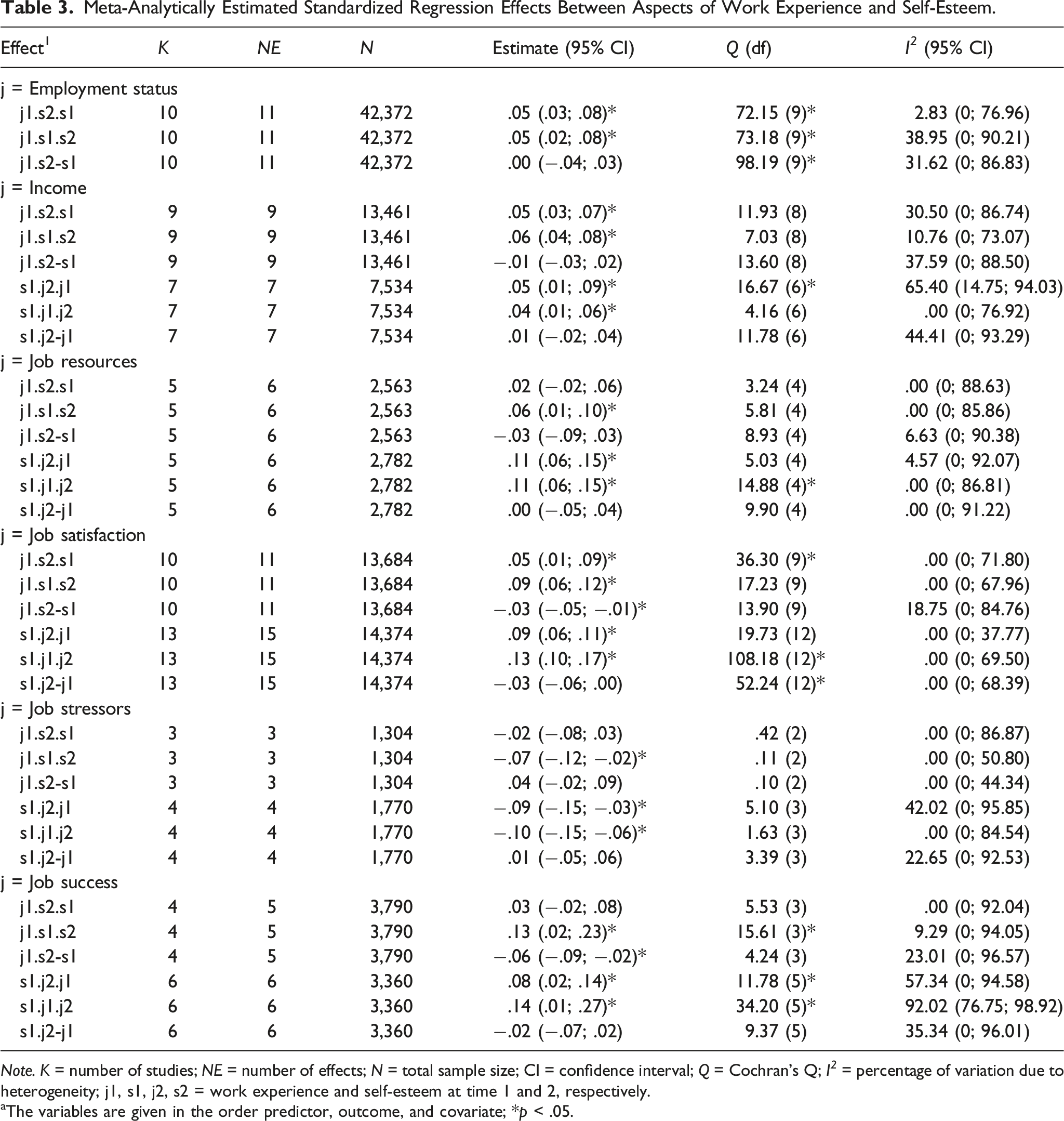
Note. K = number of studies; NE = number of effects; N = total sample size; CI = confidence interval; Q = Cochran’s Q; I² = percentage of variation due to heterogeneity; j1, s1, j2, s2 = work experience and self-esteem at time 1 and 2, respectively.

^aThe variables are given in the order predictor, outcome, and covariate; *p < .05.

Spuriousness of the effects is illustrated in Figure 4 with predicted job satisfaction and self-esteem. High initial job satisfaction predicted a subsequent increase in self-esteem if adjusting for initial self-esteem (panel A), and vice versa (panel D). Contrarily, high initial job satisfaction predicted a subsequent decrease in self-esteem if adjusting for subsequent self-esteem (panel B), and vice versa (panel E). Unadjusted effects predicted high initial self-esteem followed by a slight decrease in self-esteem for those with high initial job satisfaction (panel C), and vice versa (panel F).

Figure 4.

Predicted initial and subsequent self-esteem (a–c) and job satisfaction (d–f) for individuals with high (Z = 1), average, and low (Z = −1) initial job satisfaction and self-esteem, respectively, when conditioning on average initial (a and d) and average subsequent (b and e) degree of the outcome, and when not conditioning (c and f).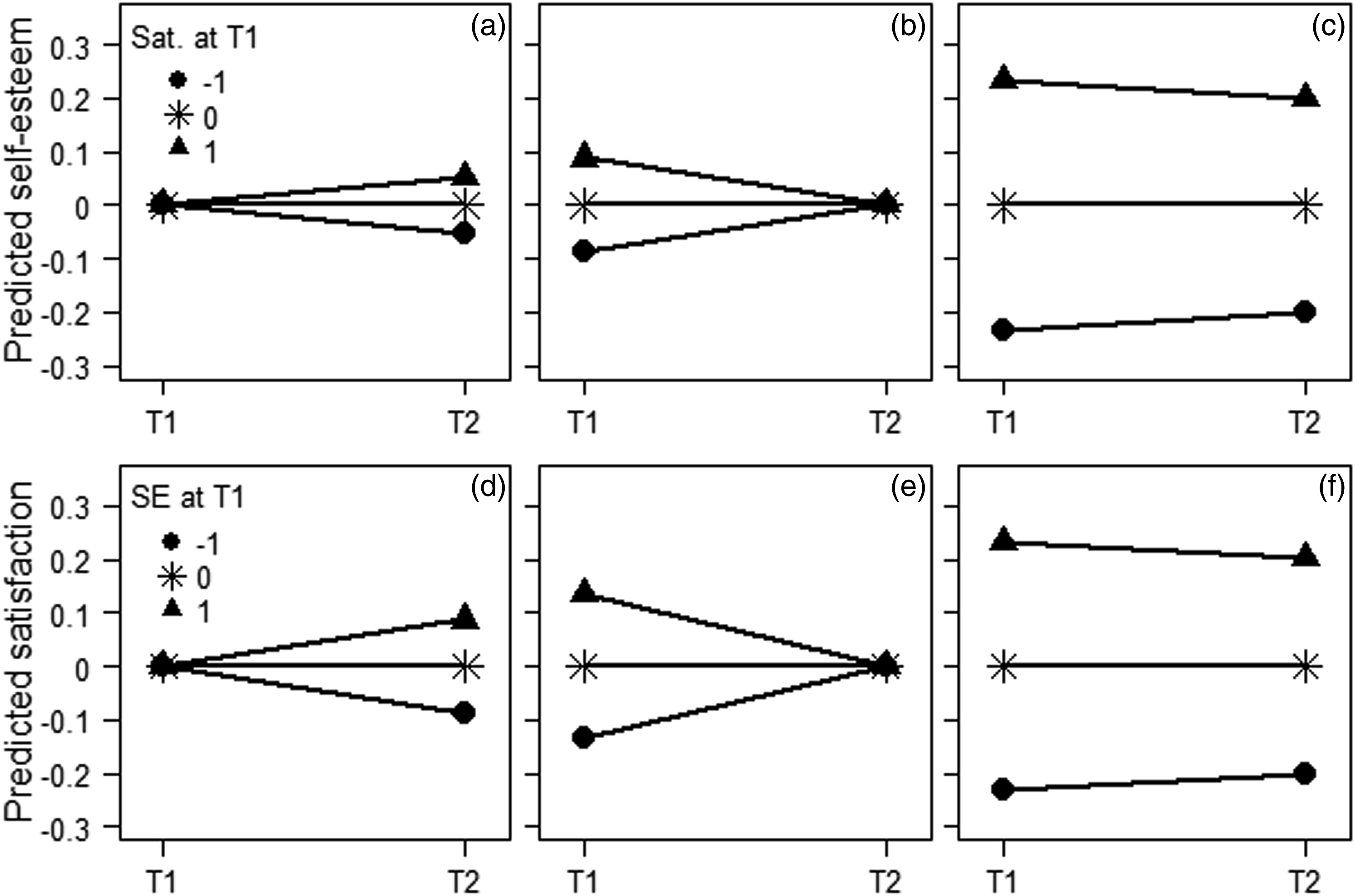

Discussion

The present meta-analytic reanalyses found prospective effects between work experiences and self-esteem to be spurious, probably due to a correlation between the predictor and residuals in the initial measurement of the outcome and regression to the mean. Effects of initial work experience on subsequent self-esteem while adjusting for initial self-esteem, and vice versa, suggested, as noted by Krauss and Orth (2022), a positive feedback loop where high self-esteem and favourable work experiences reinforced each other. However, effects of initial work experience on initial self-esteem while adjusting for subsequent self-esteem or on the unadjusted subsequent change in self-esteem, and vice versa, suggested, contrarily, no or even undermining influences between favourable work experiences and self-esteem. These contradictory findings indicated that the effects were probably spurious.

As an example, picture two individuals, A and B, with the same initial job satisfaction but A having higher initial self-esteem compared with B. Due to a positive association between job satisfaction and self-esteem, which could be due to confounding by a third variable, we may suspect that A has received a lower satisfaction score than she should, that is, experienced a negative residual, or that B has received a higher score than she should, that is, experienced a positive residual. However, as residuals tend to regress toward a mean value of zero between measurements, we should expect a more positive, but spurious, subsequent change in job satisfaction for A compared with B.

In more technical terms, if data is generated as in Figure 3, there are no true reciprocal effects between self-esteem and job satisfaction. Expected correlations between initial self-esteem and general/true job satisfaction, between initial self-esteem and initial job satisfaction, and between general/true and initial job satisfaction would equal a²b, a²bc, and c, respectively. If we plug these values into the equation for partial correlation (Cohen et al., 2003), the expected partial correlation between initial self-esteem and general/true job satisfaction while adjusting for initial job satisfaction would equal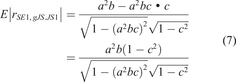

E | r_{S E 1, g J S . J S 1} | = \frac{a^{2} b - a^{2} b c ∙ c}{\sqrt{1 - {(a^{2} b c)}^{2}} \sqrt{1 - c^{2}}} = \frac{a^{2} b (1 - c^{2})}{\sqrt{1 - {(a^{2} b c)}^{2}} \sqrt{1 - c^{2}}}

(7)

If we assume that all three effects a, b, and c in Figure 3 are between (but do not include) 0 and 1, both the numerator and denominator in equation (7) would also be between (but not include) 0 and 1 and, consequently, the expected partial correlation between initial self-esteem and general/true job satisfaction while adjusting for initial job satisfaction would be a value between (but not include) 0 and 1. Moreover, as residual = observed score – true score, if the partial correlation between initial self-esteem and general/true job satisfaction while adjusting for initial job satisfaction is positive (between 0 and 1), the partial correlation between initial self-esteem and the residual in the measurement of job satisfaction while adjusting for initial job satisfaction would be negative (between −1 and 0). Consequently, we would expect, as mentioned above, a more positive, but spurious, subsequent change in job satisfaction for those with high initial self-esteem compared with those with the same initial job satisfaction but with lower initial self-esteem.

There is an ongoing debate whether, and when, it is more appropriate to analyze longitudinal data with ANOVA (corresponding to analyzing difference scores, as in Figure 4, panels C and F) or ANCOVA (corresponding to analyzing residualized values on the outcome, as in Figure 4, panels A, B, D, and E) (e.g. Kim & Steiner, 2021; Köhler et al., 2021; Lord, 1967; Lüdtke & Robitzsch, 2020; Van Breukelen, 2006). In the present case, if siding with ANOVA, the conclusion would be that there were no reciprocal effects between self-esteem and work experiences (with two exceptions, the effects on difference scores in Table 3 are non-significant).

However, it has been argued that if data is generated as in the model in Figure 5 (which assumes a true effect of X on Y2 when adjusting for Y1 and unobserved confounders), an unbiased estimate of the effect of X on the Y2-Y1 difference would require that the effect of unobserved confounders (UC) on Y1 equal the sum of the effect of these unobserved confounders on Y2 and the effect of UC on Y1 multiplied by the effect of Y1 on Y2 (i.e. that u1 = u2 + u1 × yy). This condition has been characterized as a stable effect of unobserved confounders with respect to Y1 and Y2 or as the common trend assumption (Lüdtke & Robitzsch, 2020). More generally, the common trend assumption states that change in the outcome variable (e.g. job satisfaction) between two measurements would be the same among treated (e.g. individuals with high initial self-esteem) and non-treated (e.g. individuals with low initial self-esteem) in the absence of treatment effect (Kim & Steiner, 2021). Furthermore, unbiased estimated effects on difference scores require no dynamic causal relationships, that is, effects of Y1 on X, which would mean that parameter yx in Figure 5 would be required to be zero (Lüdtke & Robitzsch, 2020).

Figure 5.

A hypothetical data generating model where unobserved confounders (UC) affect a predictor X and an outcome variable Y measured on two occasions (Y₁ and Y₂). Initial value on Y has an effect on X and both Y₁ and X have an effect on Y₂. Adapted from Lüdtke and Robitzsch (2020).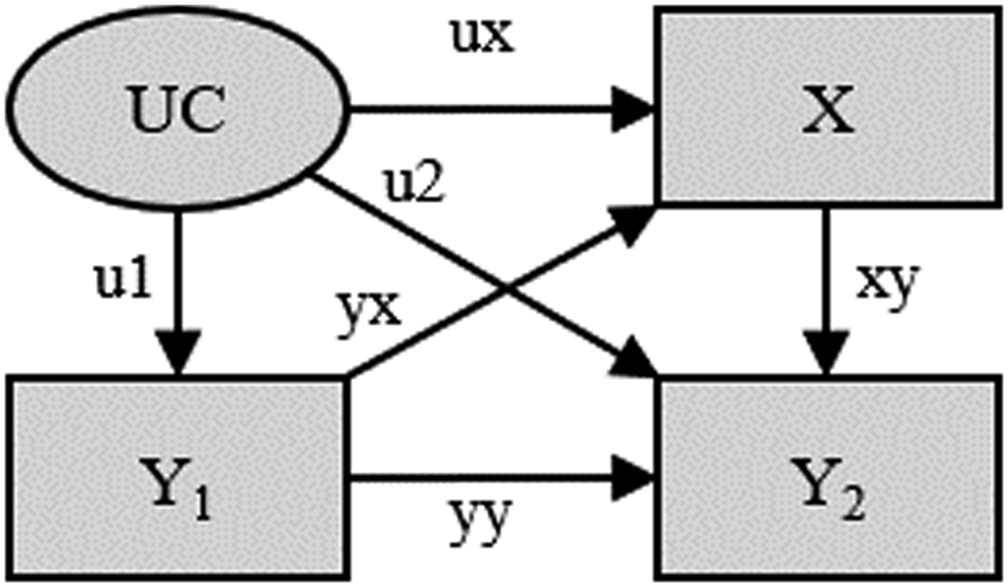

We can, of course, not guarantee that the assumptions of common trends and no dynamic causal relationships were met in all studies included in the meta-analysis by Krauss and Orth (2022) and in the present reanalysis. Consequently, it would be justified to doubt the present negative findings of no effects of self-esteem on work experience difference scores and vice versa (at least if data in the included studies were generated as in the model in Figure 5, which assumes a true effect of X on Y2 when adjusting for Y1 and unobserved confounders). However, weak evidence for negative findings do not automatically translate to strong evidence for positive findings. As an analogy, a negative indication by a suboptimal pregnancy test does not prove pregnancy.

If not trusting the findings from the difference-score ANOVA models, we may turn to the two ANCOVA models. These indicated simultaneous reinforcing and degrading reciprocal prospective effects between self-esteem and work experiences. However, we do not think that it would be tenable to conclude that self-esteem and work experiences had simultaneous reinforcing and degrading prospective effects on each other. Instead, we note that findings agreed with a situation where data have been generated without any true reciprocal effects between self-esteem and work experiences (as illustrated in Figure 3) and conclude that the observed reciprocal effects were probably spurious due to a correlation between the predictor and residuals in the initial measurement of the outcome and regression to the mean.

The model in Figure 3 is hypothetical and we can, of course, not know the true data generating model. However, neither could Krauss and Orth (2022) know that their meta-analytic data had been generated by a model including a true reciprocal reinforcing effect between self-esteem and work experiences. The model in Figure 3, without any true prospective effects, agreed better than claims by Krauss and Orth with the empirical findings of apparently simultaneous reinforcing and degrading prospective effects. Consequently, we believe that our conclusion of spurious prospective effects due to a correlation between the predictor and residuals in the initial measurement of the outcome and regression to the mean is better supported than Krauss and Orth’s conclusion of reinforcing prospective effects.

Some of our estimations differed slightly from those by Krauss and Orth (2022). For example, our meta-analytic estimation of the effect of initial self-esteem on subsequent job resources when adjusting for initial job resources was β = .11 (95% CI: .06; .15), while the corresponding value in Krauss and Orth was β = .10 (95% CI: .05; .15). This discrepancy could be due to slight differences in exactly how the meta-analytic estimations were carried out (there are some degrees of freedom involved in these analyses). Such small differences could also be due to rounding. We used correlations made available by Krauss and Orth, but we do not know how many decimal places they used for the estimated regression effects that were meta-analyzed. It should be noted that it is very unlikely that these small discrepancies could explain the paradoxical and probably spurious findings in the present reanalyses. As a sensitivity check, we can note, for example, that the non-weighted mean estimated effect of initial self-esteem on initial job resources when adjusting for subsequent job resources was β = .11 (95% CI: .04; .18), while the corresponding sample size weighted mean was β = .10 (95% CI: .04; .16). These values are very close to the meta-analytically estimated effect of β = .11 (95% CI: .06; .15). As argued above, for a true prospective increasing effect of self-esteem on job resources, this effect would be expected to be negative. It would be very surprising if a meta-analysis found a significant negative effect when the average effect is significantly positive.

We have conducted several reanalyses of meta-analyses with estimations of prospective cross-lagged effects while adjusting for a prior measure of the outcome variable (Sorjonen & Melin, 2023a, 2023b, 2023c, 2023d, 2023e, 2023f; Sorjonen et al., 2022a, 2022b; Sorjonen at al., 2023a; Sorjonen et al., 2022c; Sorjonen et al., 2023b). A recurrent message in our reanalyses is that adjusted cross-lagged effects seldom prove anything over and above a cross-sectional association combined with less than perfect reliability in measurements. This limitation is not alleviated by aggregating several cross-lagged effects in a meta-analysis. Moreover, the cross-sectional association could be due to confounding by a third variable, for example, a general positivity-negativity trait. This limitation of cross-lagged effects, as of correlations in general, is important for researchers to bear in mind in order not to overinterpret findings, something that appears to have happened to Krauss and Orth (2022). The continued output of studies with uncritical use of cross-lagged panel analyses suggests that knowledge of this limitation is lacking in the research community. Hence, continued reiteration of this fact is warranted. We recommend researchers to conduct analyses with a reversed treatment of time, as we have done here, in order to discriminate between “not yet disproven” and spurious increasing or decreasing prospective effects.

Limitations

The present reanalyses suffered from some of the same limitations as the original study by Krauss and Orth (2022). For example, 29 of 30 included samples were from a Western cultural context, with the remaining sample from Japan. Hence, it is unclear if the present main finding, that prospective effects between self-esteem and work experiences appear to be spurious due to a correlation between the predictor and residuals in the initial measurement of the outcome and regression to the mean, is generalizable to other cultural contexts.

The measurements of self-esteem and work experiences in the included studies may not always have been optimal. Moreover, we did not consider possibly moderating effects of age and sex composition of the samples, time lag between measurements, etc. However, it is important to bear in mind that such factors were constant across the analyzed models. Consequently, such factors cannot explain why the models indicated incongruent simultaneous reinforcing and undermining effects between self-esteem and work experiences.

It has been argued that analyses of data from three or more waves of measurement with, for example, random intercept cross-lagged panel models (RI-CLPM, Hamaker et al. (2015)) allow stronger inferences about causality compared with analyses of data from two waves of measurement with a traditional cross-lagged panel model (however, see Sorjonen et al. (2023c) for indications that findings from RI-CLPM may be spurious in a similar way as findings from traditional CLPM). See, for example, Lüdtke and Robitzsch (2022), Orth et al. (2021), and Usami et al. (2019) for overviews of models that can be used to analyze longitudinal data. However, in the present study, we analyzed meta-analytic data from two waves of measurement because that was the data used in the reanalyzed meta-analysis by Krauss and Orth (2022). It is possible that studies with data from many waves of measurement, hence allowing stronger inference, would show prospective effects between self-esteem and work experiences that would be more difficult to refute as spurious. The point of the present reanalysis is not primarily to claim that true prospective effects between self-esteem and work experiences do not exist. The main point is, rather, that the existence of such prospective effects has not been proven by the meta-analysis by Krauss and Orth (2022).

Conclusions

The present reanalysis of a meta-analysis by Krauss and Orth (2022) found incongruent simultaneous reinforcing and undermining prospective cross-lagged effects between self-esteem and work experiences. Consequently, the prospective effects appeared to be spurious due to a correlation between the predictor and residuals in the initial measurement of the outcome and regression to the mean rather than, as suggested by Krauss and Orth, due to a positive feedback loop where high self-esteem and favourable work experiences reinforced each other. It is important for researchers to be aware of the limitations of cross-lagged effects in order not to overinterpret findings.

Footnotes

Acknowledgements

We thank Krauss and Orth (2022) for making their meta-analytic data, reanalyzed in the present study, available at the Open Science Framework at .

Declaration of conflicting interests

The author(s) declared no potential conflicts of interest with respect to the research, authorship, and/or publication of this article.

Funding

The author(s) received no financial support for the research, authorship, and/or publication of this article.

Open science statements

(1) Data, a list of studies included in the meta-analyses, forest-plots, and an analysis script are available at the Open Science Framework at https://osf.io/p2ect/; (2) Our hypotheses were not preregistered; (3) We did not conduct any power analyses and sample sizes were given by the studies included in the meta-analysis by ; (4) The meta-analytic data analyzed in the present reanalyses have previously been analyzed by Krauss and Orth (2022); (5) In the present reanalyses, we included prior measures of the outcome variable, self-esteem and work experience, as covariates. We did this in order to follow the procedure by Krauss and Orth (2022) and because this is common practice in cross-lagged panel analyses; (6) As it was not vital for the objective of the present study and in order to save space, we do not report basic descriptive statistics for the studies included in the present re-meta-analysis. Some information, for example, on the sex composition and mean age of participants in the included studies, is available in Krauss and Orth (2022).

ORCID iD

Kimmo Sorjonen

References

Castro-Schilo

Grimm

K. J.

(2018). Using residualized change versus difference scores for longitudinal research. Journal of Social and Personal Relationships, 35(1), 32–58. https://doi.org/10.1177/0265407517718387

Cohen

West

S. G.

Aiken

L. S.

(2003). Applied multiple regression/correlation analysis for the behavioral sciences (3rd ed.). Lawrence Erlbaum Associates.

Eriksson

Häggström

(2014). Lord’s paradox in a continuous setting and a regression artifact in numerical cognition research. PLoS One, 9(4), Article e95949. https://doi.org/10.1371/journal.pone.0095949

Glymour

M. M.

Weuve

Berkman

L. F.

Kawachi

Robins

J. M.

(2005). When is baseline adjustment useful in analyses of change? An example with education and cognitive change. American Journal of Epidemiology, 162(3), 267–278. https://doi.org/10.1093/aje/kwi187

Guilford

J. P.

(1965). Fundamental statistics in psychology and education (4th ed.). McGraw-Hill.

Hamaker

E. L.

Kuiper

R. M.

Grasman

R. P. P. P.

(2015). A critique of the cross-lagged panel model. Psychological Methods, 20(1), 102–116. https://doi.org/10.1037/a0038889

Kim

Steiner

P. M.

(2021). Gain scores revisited: A graphical models perspective. Sociological Methods & Research, 50(3), 1353–1375. https://doi.org/10.1177/0049124119826155

Köhler

Hartig

Schmid

(2021). Deciding between the covariance analytical approach and the change-score approach in two wave panel data. Multivariate Behavioral Research, 56(3), 447–458. https://doi.org/10.1080/00273171.2020.1726723

Krauss

Orth

(2022). Work experiences and self-esteem development: A meta-analysis of longitudinal studies. European Journal of Personality, 36(6), 849–869. https://doi.org/10.1177/08902070211027142

10.

Lord

F. M.

(1967). A paradox in the interpretation of group comparisons. Psychological Bulletin, 68(5), 304–305. https://doi.org/10.1037/h0025105

11.

Lüdtke

Robitzsch

(2020). ANCOVA versus change score for the analysis of nonexperimental two-wave data: A structural modeling perspective. Preprint, 12 September. PsyArXiv. https://doi.org/10.31234/osf.io/5zdmes

12.

Lüdtke

Robitzsch

(2022). A comparison of different approaches for estimating cross-lagged effects from a causal inference perspective. Structural Equation Modeling: A Multidisciplinary Journal, 29(6), 888–907. https://doi.org/10.1080/10705511.2022.2065278

13.

Orth

Clark

D. A.

Donnellan

M. B.

Robins

R. W.

(2021). Testing prospective effects in longitudinal research: Comparing seven competing cross-lagged models. Journal of Personality and Social Psychology, 120(4), 1013–1034. https://doi.org/10.1037/pspp0000358

14.

R Core Team . (2022). R: A language and environment for statistical computing. R Foundation for Statistical Computing. URL. https://www.R-project.org/

15.

Sorjonen

Ingre

Melin

Nilsonne

(2022b). Questioning the reciprocal effects model of academic self-concept and achievement: A reanalysis of a meta-analysis of longitudinal studies and a simulation. Preprint, 6 October. PsyArXiv. https://doi.org/10.31234/osf.io/qd4bj

16.

Sorjonen

Ingre

Melin

Nilsonne

(2022a). Prospective associations between self-esteem and quality of social relations may be spurious: Reanalysis of a meta-analysis of longitudinal studies. Preprint, 26 December. PsyArXiv. https://doi.org/10.31234/osf.io/kusft

17.

Sorjonen

Melin

(2023a). Prospective associations between social support and posttraumatic stress disorder may be spurious: A re-meta-analysis of longitudinal studies and a simulation. Journal of Affective Disorders, 340, 174–180. https://doi.org/10.1016/j.jad.2023.08.014

18.

Sorjonen

Melin

(2023b). Spurious prospective associations between unemployment and wellbeing: Reanalysis of a meta-analytic cross-lagged panel analysis. Preprint, 23 March. PsyArXiv. https://doi.org/10.31234/osf.io/b3pgh

19.

Sorjonen

Melin

(2023c). Spurious prospective effect of perfectionism on depression: Reanalysis of a meta-analytic cross-lagged panel analysis. Preprint, 20 April. PsyArXiv. https://doi.org/10.31234/osf.io/rfs3u

20.

Sorjonen

Melin

(2023d). Spurious prospective effect of self-efficacy on academic performance: Reanalysis of a meta-analytic cross-lagged panel analysis. Preprint, 10 march. PsyArXiv. https://doi.org/10.31234/osf.io/qgcu5

21.

Sorjonen

Melin

(2023e). Spurious prospective effects between general and domain-specific self-esteem: A reanalysis of a meta-analysis of longitudinal studies. Preprint, 25 April. PsyArXiv. https://doi.org/10.31234/osf.io/w5sf8

22.

Sorjonen

Melin

(2023f). Spurious prospective effects of mindfulness on anxiety and depressive symptoms: Reanalysis of a meta-analytic cross-lagged panel analysis. Preprint, 5 May. PsyArXiv. https://doi.org/10.31234/osf.io/c34w8

23.

Sorjonen

Melin

Ingre

(2019). Predicting the effect of a predictor when controlling for baseline. Educational and Psychological Measurement, 79(4), 688–698. https://doi.org/10.1177/0013164418822112

24.

Sorjonen

Melin

(2023a). Spurious prospective effects between work experiences and self-esteem: A reanalysis of a meta-analysis of longitudinal studies. Preprint, 12 April. PsyArXiv. https://doi.org/10.31234/osf.io/n9aj3

25.

Sorjonen

Nilsonne

Ingre

Melin

(2022c). Questioning the vulnerability model: Prospective associations between low self-esteem and subsequent depression ratings may be spurious. Journal of Affective Disorders, 315, 259–266. https://doi.org/10.1016/j.jad.2022.08.003

26.

Sorjonen

Nilsonne

Melin

(2023b). Spurious peer influence: Reanalysis of a meta-analysis of longitudinal studies. Preprint, 24 February. PsyArXiv. https://doi.org/10.31234/osf.io/szkt8

27.

Sorjonen

Nilsonne

Melin

Ingre

(2023c). Uncertain inference in random intercept cross-lagged panel models: An example involving need for cognition and anxiety and depression symptoms. Personality and Individual Differences, 201(4), 111925. https://doi.org/10.1016/j.paid.2022.111925

28.

Usami

Murayama

Hamaker

E. L.

(2019). A unified framework of longitudinal models to examine reciprocal relations. Psychological Methods, 24(5), 637–657. https://doi.org/10.1037/met0000210

29.

Van Breukelen

G. J. P.

(2006). ANCOVA versus change from baseline had more power in randomized studies and more bias in nonrandomized studies. Journal of Clinical Epidemiology, 59(9), 920–925. https://doi.org/10.1016/j.jclinepi.2006.02.007

30.

Viechtbauer

(2010). Conducting meta-analyses in R with the metafor package. Journal of Statistical Software, 36(3), 1–48. https://doi.org/10.18637/jss.v036.i03