Sage Journals: Discover world-class research

Abstract

This article is part of a Journal of Biological Rhythms series exploring analysis and statistics topics relevant to researchers in biological rhythms and sleep research. The goal is to provide an overview of the most common issues that arise in the analysis and interpretation of data in these fields. In this article on time series analysis for biological rhythms, we describe some methods for assessing the rhythmic properties of time series, including tests of whether a time series is indeed rhythmic. Because biological rhythms can exhibit significant fluctuations in their period, phase, and amplitude, their analysis may require methods appropriate for nonstationary time series, such as wavelet transforms, which can measure how these rhythmic parameters change over time. We illustrate these methods using simulated and real time series.

Keywords

time-frequency analysis wavelet transform biological rhythms mathematical analyses circadian rhythms

Measuring the period and other rhythmic parameters of biological rhythms can often be quite challenging. What methods for assessing rhythms work best can depend on the type of data (e.g., locomotor activity, body temperature, bioluminescence recordings, etc.) as well as on the length of recording, sampling rate, waveform, and rhythmic properties of the particular time series. When time series are quite noisy with fluctuating period and amplitude, their analysis may require methods appropriate for nonstationary time series. We recommend starting with simpler methods and then progressing to more complex methods when needed. The advice given in the first article of this series (Bianchi et al., 2017) absolutely holds here as well: Make a habit of plotting data. Particularly when time series data are noisy or cover only a few cycles, period and phase estimation methods can easily produce poor results if not handled carefully. Visual checking to ensure that results are consistent with the data will guard against erroneous conclusions. Applying two or more independent methods and comparing the results can also catch potential problems.

In the second article of this series, Klerman et al. (2017) provide an overview of common methods and issues involved in longitudinal analysis of biological rhythms data, particularly when the data can be “folded” into day-length windows and overlapped for analysis. In this article, we consider alternative methods that can work well for time series with fluctuations in period, phase, and amplitude. We also discuss preprocessing of time series to remove trend as well as testing for significant rhythmicity before proceeding to estimate period and phase. We demonstrate methods that can be useful for a deeper analysis of nonstationary time series (i.e., records for which the rhythmic parameters such as period, amplitude, and phase might not be constant over the duration of the record). For a discussion of nonstationary time series arising in circadian research, see Refinetti (2004).

Methods appropriate for analysis of microarray data and other situations where only 1 or 2 cycles are available will not be addressed here; see Wu et al. (2016) for appropriate methods. This article will focus on methods appropriate to time series containing at least 3 full cycles (preferably more), where the data were collected from a single individual over time. Increasing the number of cycles present in the time series has a much greater effect in improving period estimates than does increasing the sampling rate (Cohen et al., 2012), so generally try to collect as many cycles of good quality data as possible.

Preprocessing of Time Series Data

Cleaning the data is always a first important step. Identify missing values in the time series and determine how to treat them. If only a few values are missing, impute them using some appropriate method (Enders, 2010). Also identify outlier values, for instance, effects of cosmic rays on bioluminescence data. Extreme outlier values should be replaced by more moderate values (e.g., treat them as missing values and impute them using some appropriate method). If there are many missing values or the sampling rate is not uniform, methods such as the Lomb-Scargle periodogram (Glynn et al., 2006) that do not require uniform sampling may be needed for estimating period. There are also newer wavelet lifting methods designed to work well for estimating period in the presence of missing or irregularly sampled data (Knight et al., 2012; Hamilton et al., 2017).

Trend Removal

If the time series exhibits a significant underlying trend, removing that trend before proceeding with testing for rhythmicity and measuring rhythmic parameters can often greatly improve the results. The goal in removing trend is to produce a steady baseline about which the time series oscillates, without distorting the period or phase of the oscillations. Options include subtracting a running average over a window at least the length of the expected period, subtracting a linear or low-degree polynomial fit to the entire time series, convolving with a filter (Levine et al., 2002), or applying a discrete wavelet transform (Leise and Harrington, 2011). Filter and transform-based methods tend to perform better with longer records that cover more than a few cycles. Polynomial fits for detrending purposes should involve only first- or second-degree polynomials; using a higher degree runs the risk of altering the properties of the rhythm itself.

Consider the example shown in Figure 1 of a noisy sinusoid with a nonlinear trend. Subtracting a second-degree polynomial fit to the data removes most of the underlying trend, while a higher degree polynomial can significantly distort the rhythm, as shown in Figure 1B. Applying a discrete wavelet transform does a better job of centering the cycles about zero but will require a loss of information at the left and right edges (to minimize edge effects, the transform should be applied to the time series starting and ending at peaks or troughs). The discrete wavelet transform can also be used to reduce noise and smooth the time series. Generally, filtering and transform-based methods work better on long records where losing some data at the start and end of the record is not problematic. For short time series with only a few cycles, subtracting a linear fit (first-degree polynomial) is typically adequate for purposes of most methods that require a detrended (or zero-centered) time series.

Figure 1.

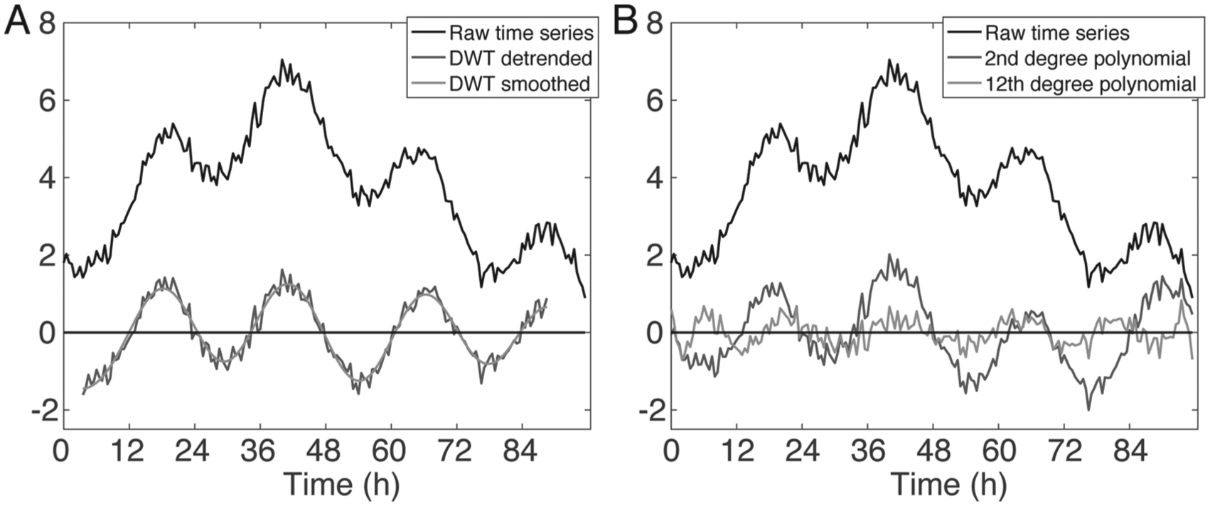
Example of a noisy sinusoid with period slightly less than 24 h and a nonlinear trend. Noise is normally distributed with mean zero and standard deviation equal to 20% of the sinusoid’s amplitude. (A) The raw time series before and after cleaning by a discrete wavelet transform (DWT), as described by Leise and Harrington (2011). (B) The raw time series before and after subtracting a fitted second-degree polynomial and 12th-degree polynomial, demonstrating that using higher order polynomials to remove trend can detrimentally alter the underlying rhythm.

Testing for Rhythmicity

Determining whether a noisy time series exhibits significant rhythmicity can be quite challenging, especially if the times series is relatively short in duration. Spikes of random noise can give a misleading appearance of rhythmicity, while stochastically fluctuating cycle lengths can cause a rhythmicity test to be negative even though a rhythm is indeed present. Commonly used rhythmicity tests include autocorrelation (Dowse, 2009), Fisher’s test for significant periodicity (Wichert et al., 2004), the Lomb-Scargle periodogram (Glynn et al., 2006), and other tests related to the discrete Fourier transform, such as that described by Leise et al. (2012). A related idea is the robustness or strength of rhythmicity, allowing a more nuanced view than whether a time series is rhythmic or arrhythmic. Methods for measuring the strength of rhythmicity include the rhythmicity index, the goodness of fit for sinusoids or other curves, and the proportion of energy associated with each frequency or frequency band in Fourier and wavelet transform methods.

Autocorrelation is the simplest of these methods and can be an excellent first method to obtain quick results on the quality of rhythms in the data if sampling is uniform and there are no missing observations. For best results, remove trend as described in the previous section before calculating the autocorrelation. The underlying idea is to compare the time series to shifted versions of itself; shifting a rhythmic time series by a full period should result in a high positive correlation. The peak value is the rhythmicity index, which will equal 1 for a perfectly periodic time series and be near zero for pure uncorrelated noise. For longer time series, the second peak in autocorrelation may provide a better index (Dowse, 2009). This rhythmicity index can be used as a simple measure of rhythmicity that is independent of waveform. Autocorrelation can also be used to detect rhythmicity but tends to be poor at this job because the test is really to determine whether the time series is significantly different from random uncorrelated noise, not whether it is rhythmic. See Figure 2 for examples of autocorrelation applied to noisy sinusoidal time series. If the signal-to-noise ratio is high, the autocorrelation function itself will appear rhythmic with the peak value (rhythmicity index) well above the significance line; in this case, the lag corresponding to the peak in autocorrelation will provide a reasonably accurate period estimate (although other methods may provide a better estimate). A low signal-to-noise ratio tends to reduce the rhythmicity index and the accuracy of the resulting period estimate, and pure noise will yield autocorrelations fluctuating about zero, a sign of arrhythmicity. Note that the rhythmicity index does not depend on the amplitude of the oscillation per se but rather on the signal-to-noise ratio. It also depends how consistently the cycle repeats itself, as changes in cycle length and waveform from cycle to cycle will decrease the rhythmicity index.

Figure 2.

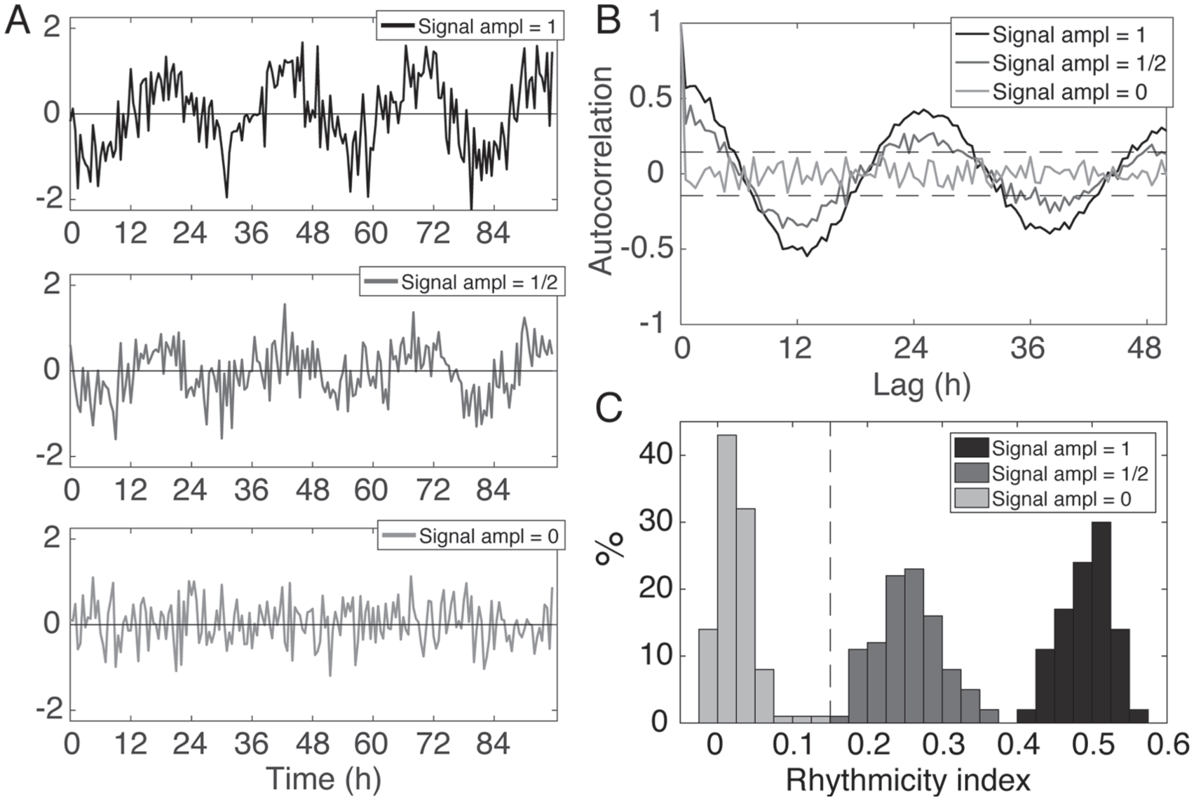
Autocorrelation applied to noisy time series. (A) Three examples of noisy time series that are the sum of a sinusoid with the indicated amplitude plus normally distributed noise with mean zero and standard deviation 0.5. (B) Graph of the autocorrelation (correlogram) for each time series. (C) Distribution of rhythmicity indices for 100 time series for each amplitude value. The dashed line indicates the α = 0.05 threshold for time series to be significantly different from noise.

Another prominent method is the Fourier periodogram, which requires many cycles to give accurate period estimates and so is often not useful for the shorter time series available in circadian research. However, it can provide an effective test for circadian rhythmicity in some situations through Fisher’s g statistic. This test indicates whether the maximum peak in the Fourier periodogram is significant, assuming the times series is composed of a sinusoidal component plus white noise (Wichert et al., 2004). For improved performance, the Fourier periodogram should be computed using a window function, such as a Blackman-Harris window, which tapers the ends of the time series to reduce edge effects. In practice, Fisher’s g statistic may not perform well if the waveform deviates from sinusoidal or the assumption of additive white noise is violated. White noise has a uniform frequency spectrum, but noise in biological data sometimes follows an inverse power law distribution (e.g., as observed by Leise et al. 2012), which provides an alternative to Fisher’s g statistic under that assumption. This alternative method tests whether the power associated with the dominant period is significantly larger than that for the background noise based on a regression line in the log-log plot of the discrete Fourier transform.

The Lomb-Scargle periodogram can provide both a test of significant rhythmicity and a period estimate (Glynn et al., 2006). Furthermore, it does not require uniform sampling in time and is robust to missing data, unlike most of the other methods discussed here (although note that fitting to curves such as sinusoids also does not require uniform sampling). The Lomb-Scargle periodogram assumes a periodic signal plus normally distributed white noise and is based on a least-squares fit of sinusoids to the data, in contrast to the Fourier periodogram that assumes a fixed set of frequencies. The associated statistic tests whether a peak in the Lomb-Scargle periodogram is due to chance or indicates significant rhythmicity at that period.

Taking waveform into account when selecting a rhythmicity test is important. If the waveform is similar to sinusoidal, then tests based on the discrete Fourier transform or fitting to sinusoids are likely to be appropriate. However, if the waveform differs from sinusoidal, such as activity data often do, these methods may not perform well. For instance, the Fourier transform of a square wave has power widely distributed across frequencies, rather than an isolated dominant peak at the period value, which can lead to misleading results for Fourier-based rhythmicity tests. A method like autocorrelation that is independent of waveform may be preferred in this situation.

A multiple testing procedure to control the false discovery rate should be applied if testing a large set of samples for significant rhythmicity. One such procedure attributable to Benjamini and Hochberg is described by Wichert et al. (2004) for controlling the false discovery rate at level q for a set of N samples, as follows. Order the p values resulting from whatever rhythmicity test was applied in increasing order: p₍₁₎, p₍₂₎, . . . , p_(N). Find the largest integer n for which p_(n) ≤ nq/N. A sample from the set is considered significantly rhythmic if p ≤ p_(n), where n is that largest integer.

See Figure 3 for these methods applied to SCN cell time series from (Liu et al., 2007). Observe that the percentage of cells judged significantly rhythmic (Figure 3C) can vary considerably depending on the method used. The rhythmicity indices shown in Figure 3D suggest that while WT cells tend to exhibit stronger rhythms than the Per1^–/– cells, there is a great deal of variability across cells in each group. One reason for the differing rhythmicity results across methods in Figure 3C is that deficits in rhythmicity vary greatly across cells. Tests differ in their sensitivity to issues like decaying amplitude, changes in waveform, and nonwhite or nonadditive noise. Furthermore, an individual cell can exhibit considerable variability in its rhythmic properties. The rhythmic time series shown in Figure 3A has a large change in amplitude as well as minor fluctuations in cycle length. For time series exhibiting both high levels of noise and large variations in period and amplitude from cycle to cycle, there may be no clean separation between clearly rhythmic cells and clearly arrhythmic cells. Where to draw the line between rhythmic and arrhythmic is difficult and depends on the test used. A more complete overview of the quality of the rhythms can be obtained by examining the distribution of some measure of the strength of rhythmicity across each group, such as the rhythmicity index, the goodness of fit for sinusoids or other appropriate waveforms, or the proportion of energy associated with the dominant frequency or frequency band in Fourier and wavelet transform methods.

Figure 3.

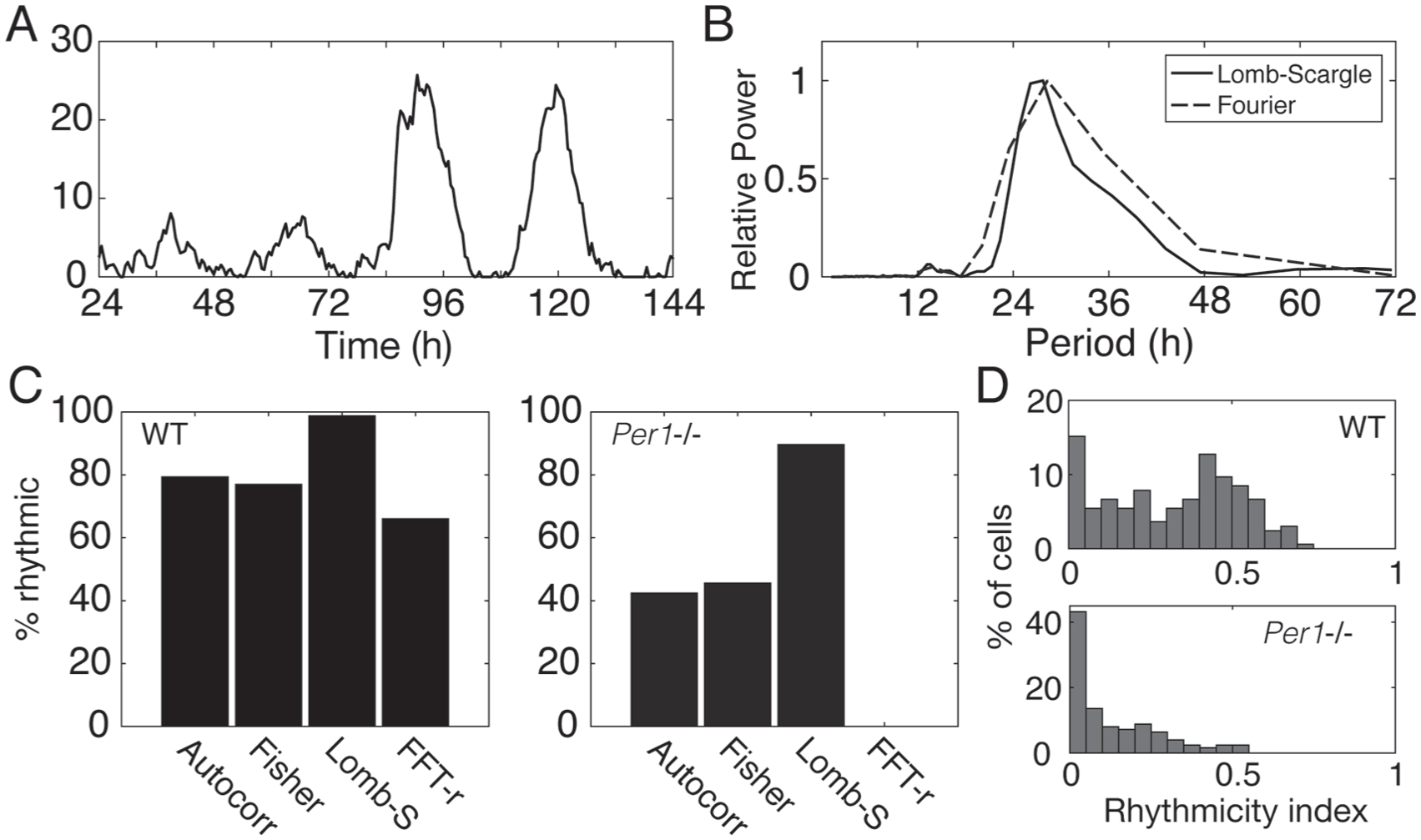
Rhythmicity tests applied to mPer2^Luc recordings of dissociated WT and Per1^–/– SCN neurons from Liu et al. (2007). (A) Example of a rhythmic WT SCN time series. (B) Lomb-Scargle and Fourier periodograms of the 5-day-long time series in A. (C) Percentage of cells in each group judged significantly rhythmic by 4 different methods: autocorrelation, Fisher’s g statistic, Lomb-Scargle periodogram, and an alternative test (FFT-r) based on regression of the log-log plot of the FFT (Leise et al., 2012). The multiple testing procedure described in the text was applied with q = 0.05. Lomb-Scargle gives the highest percent rhythmic for both groups of cells, and the FFT-r gives the lowest, with none of the mutant cells deemed rhythmic by that test. (D) Distribution of rhythmicity index for each group of cells, indicating strength of rhythmicity. Mean ± standard deviation is 0.31 ± 0.22 for WT and 0.09 ± 0.19 for Per1^–/– SCN neurons.

Measuring Period, Phase, and Amplitude

A wide range of methods have been developed for the purpose of estimating the period, phase, and amplitude of biological rhythms, including fitting sinusoids or other curves appropriate to the typical waveform of the time series, such as 1- or 2-component cosinor (Cornélissen, 2014), as well as the Fourier periodogram (Welch, 1967), the Lomb-Scargle periodogram (Glynn et al., 2006), and MESA (Dowse, 2009). Also see Refinetti et al. (2007) and Zielinski et al. (2014) for reviews of period estimation methods. Whatever the method, accuracy in estimating period, phase, and amplitude depends on both the number of cycles and the sampling rate. Increasing the number of cycles present in the time series tends to have a much greater effect in improving period estimates than does increasing the sampling rate, and uncertainty in the estimates tends to be high if the time series covers only a few cycles (Cohen et al., 2012). The highest frequency that can be detected is the Nyquist frequency, which equals half the sampling rate. For example, if samples are taken twice an hour, then 1 hour is the shortest period that can be detected.

The methods mentioned above cannot measure changes in period or other rhythmic parameters over time. To calculate how oscillations vary over time, time-frequency methods should be applied, which include spectrograms and discrete and continuous wavelet transforms (Leise, 2015) and other transforms such as the Hilbert transform (Boashash, 1992), empirical mode decomposition and the Hilbert-Huang transform (Huang, 2014), and nonlinear mode decomposition (Iatsenko et al., 2015). See Torrence and Compo (1998), Selesnick et al. (2005), and Quotb et al. (2011) for general guides to wavelet analysis. Further applications of wavelets include computation of phase relationships and coherence between 2 oscillations (Grinsted et al., 2004) and of phase-amplitude interactions between circadian and ultradian components of a times series (Thengone et al., 2016). Here we will focus on illustrating basic wavelet-based methods to assess nonstationary circadian time series exhibiting fluctuations in period, phase, and amplitude.

The discrete wavelet transform decomposes a time series into components associated with different frequency bands, determined by the sampling rate (Percival and Walden, 2000). Nonlinear and empirical mode decompositions similarly decompose a time series into distinct components using different methods (Huang, 2014; Iatsenko et al., 2015); these methods do not produce the same results as a discrete wavelet transform but can be similar in nature. The waveform of the components produced by a wavelet transform depends on the wavelet used, while the waveform associated with empirical mode decomposition is determined by the time series itself. Figure 4 provides an example of a long PER2::LUC recording of a mouse fibroblast that exhibits fluctuations in amplitude and period (mice expressing PER2::LUC bioluminescence provide a means to measure intracellular Period2 clock gene expression; Welsh et al., 2004). Figure 4B compares the circadian components found by applying a discrete wavelet transform and nonlinear mode decomposition.

Figure 4.

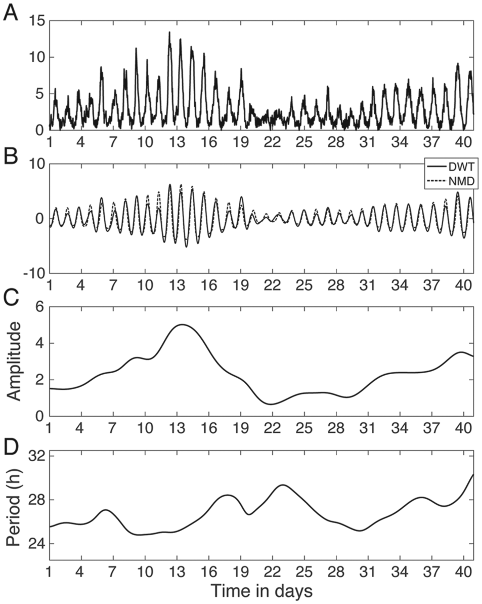
Methods for nonstationary time series applied to a rhythm in clock gene expression. (A) PER2::LUC recording of a mouse fibroblast in photons per minute from Leise et al. (2012). (B) The circadian components found by two methods, a discrete wavelet transform (DWT) and nonlinear mode decomposition (NMD). An analytic wavelet transform was also applied to obtain the amplitude, shown in C, and the period, shown in D, varying over time, calculated as described by Leise and Harrington (2011).

A continuous wavelet transform provides information about what frequencies are most dominant at each time point and so can be used to estimate amplitude, period, and phase varying over time (Mallat, 2009). A continuous wavelet transform using an analytic wavelet function can produce particularly good results (Lilly and Olhede, 2010). Figure 4C shows the amplitude of the fibroblast example over time, and Figure 4D shows the period changing over time, as estimated by an analytic wavelet transform. As an example of a wavelet method applied to activity data, Figure 5 shows the analytic wavelet transform of a female mouse wheel-running record, displaying a clear 5-day pattern of fluctuation in period, phase, and amplitude. The strongest band in the scalogram in Figure 5B is around a 24-h period, but also note the 5-day pattern in the region between 12 and 18 h caused by the scalloping pattern in nighttime activity.

Figure 5.

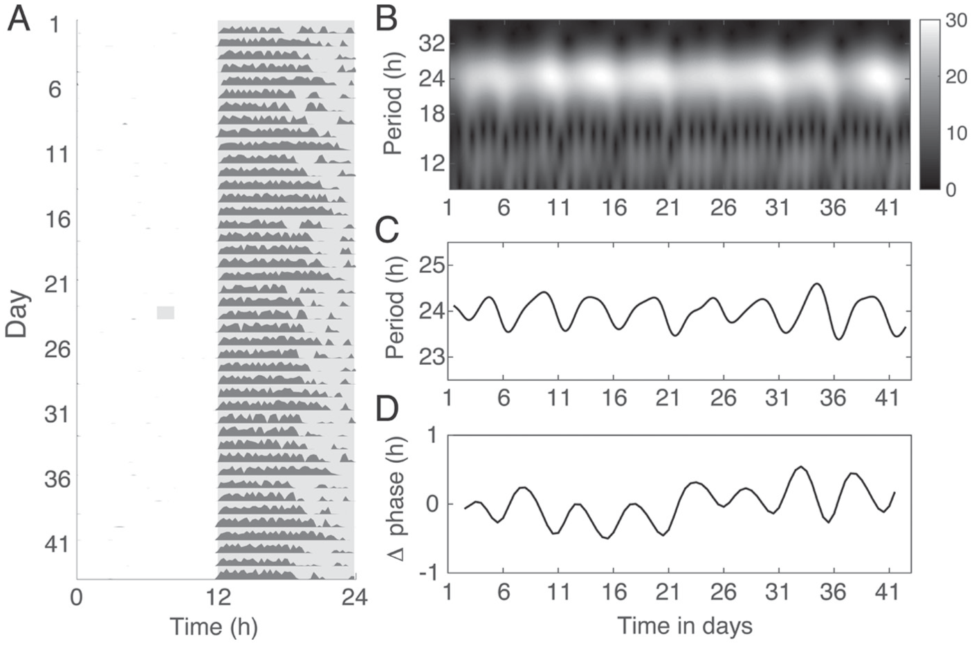
Methods for nonstationary time series applied to a wheel-running record of a female mouse. (A) Actogram displaying activity of a female mouse under a 12:12 light-dark cycle from the study described by Leise and Harrington (2011). (B) Scalogram of an analytic wavelet transform applied to the activity record, revealing a 5-day pattern in period (C) and phase (D) due to the estrous cycle. The grayscale value in the scalogram indicates the amplitude of the rhythm, in wheel revolutions per minute, calculated as described by Leise and Harrington (2011).

Concluding Remarks

Methods to extract period, phase, and amplitude over time can be delicate calculations, sensitive to missing data and other disruptions in the record. While some time-frequency methods like continuous wavelet transforms find the “instantaneous frequency” at each time point, the estimate actually incorporates information from a time frame typically at least 3 days wide (period cannot be estimated from a single data point!). Therefore these methods tend to produce the most useful results about circadian rhythms from records that are at least 5 days long with no missing data. In general, other more traditional methods should be applied first to obtain a general sense of the rhythmic properties of the data before turning to the more nuanced but also more finicky time-frequency methods like wavelet transforms.

The author maintains a website providing MATLAB scripts for applying the wavelet transforms and some other analyses described in this article: http://www3.amherst.edu/~tleise/CircadianWaveletAnalysis.html.

References

Bianchi

Phillips

AJK

Wang

Klerman

(2017) Statistics for sleep and biological rhythms research: from distributions and displays to correlation and causation. J Biol Rhythms 32:7-17.

Boashash

(1992) Estimating and interpreting the instantaneous frequency of a signal, I: fundamentals. Proc IEEE 80:520-538.

Cohen

Leise

Welsh

(2012) Bayesian statistical analysis of circadian oscillations in fibroblasts. J Theor Biol 314:182-191.

Cornélissen

(2014) Cosinor-based rhythmometry. Theoretical Biology and Medical Modelling 11:16.

Dowse

(2009) Analyses for physiological and behavioral rhythmicity. Methods Enzymol 454:141-174.

Enders

(2010) Applied Missing Data Analysis. New York: Guilford Press.

Glynn

Chen

Mushegian

(2006) Detecting periodic patterns in unevenly spaced gene expressiontime series using Lomb–Scargle periodograms. Bio-informatics 22:310-316.

Grinsted

Moore

Jevrejeva

(2004) Application of the cross wavelet transform and wavelet coherence to geophysical time series. Nonlinear Process Geophys 11:561-566.

Hamilton

Nunes

Knight

Fryzlewicz

(2017) Complex-valued wavelet lifting and applications. Technometrics.

10.

Huang

(2014) Hilbert-Huang Transform and Its Applications. Singapore: World Scientific.

11.

Iatsenko

McClintock

Stefanovska

(2015) Nonlinear mode decomposition: a noise-robust, adaptive decomposition method. Phys Rev E 92:032916.

12.

Klerman

Wang

Phillips

AJK

Bianchi

(2017) Statistics for sleep and biological rhythms research: longitudinal analysis of biological rhythms data. J Biol Rhythms 32:18-25.

13.

Knight

Nunes

Nason

(2012) Spectral estimation for locally stationary time series with missing observations. Stat Comput 22:877-895.

14.

Leise

Wang

Gitis

Welsh

(2012) Persistent cell-autonomous circadian oscillations in fibroblasts revealed by six-week single-cell imaging of PER2::LUC bioluminescence. PLoS One 73:e33334.

15.

Leise

(2015) Wavelet-based analysis of circadian behavioral rhythms. Methods Enzymol 551:95-119.

16.

Leise

Harrington

(2011) Wavelet-based time series analysis of circadian rhythms. J Biol Rhythms 26:454-463.

17.

Levine

Funes

Dowse

Hall

(2002) Signal analysis of behavioral and molecular cycles. BMC Neurosci 3:1.

18.

Lilly

Olhede

(2010) On the analytic wavelet transform. IEEE Trans Inf Theory 56:4135-4156.

19.

Liu

Welsh

Tran

Zhang

Meeker

Takahashi

(2007) Intercellular coupling confers robustness against mutations in the SCN circadian clock network. Cell 129:605-616.

20.

Mallat

(2009) A Wavelet Tour of Signal Processing: The Sparse Way. Burlington, MA: Academic Press.

21.

Percival

Walden

(2000) Wavelet Methods for Time Series Analysis. New York: Cambridge University Press.

22.

Quotb

Bornat

Renaud

(2011) Wavelet transform for real-time detection of action potentials in neural signals. Front Neuroeng 4:7.

23.

Refinetti

(2004) Non-stationary time series and the robustness of circadian rhythms. J Theor Biol 227:571-581.

24.

Refinetti

Cornélissen

Halberg

(2007) Procedures for numerical analysis of circadian rhythms. Biol Rhythm Res 38:275-325.

25.

Selesnick

Baraniuk

Kingsbury

(2005) The dual-tree complex wavelet transform. IEEE Signal Process Mag 22:123-151.

26.

Thengone

Gagnidze

Pfaff

Proekt

(2016) Phase-amplitude coupling in spontaneous mouse behavior. PloS One 11:e0162262.

27.

Torrence

Compo

(1998) A practical guide to wavelet analysis. Bull Am Meteorol Soc 69:61-78.

28.

Welch

(1967) The use of fast Fourier transform for the estimation of power spectra: a method based on time averaging over short, modified periodograms. IEEE Transactions on Audio and Electroacoustics 15:70-73.

29.

Welsh

Yoo

S-H

Liu

Takahashi

Kay

(2004) Bioluminescence imaging of individual fibroblasts reveals persistent, independently phased circadian rhythms of clock gene expression. Curr Biol 14:2289-2295.

30.

Wichert

Fokianos

Strimmer

(2004) Identifying periodically expressed transcripts in microarray time series data. Bioinformatics 20:5-20.

31.

Anafi

Hughes

Kornacker

Hogenesch

(2016) MetaCycle: an integrated R package to evaluate periodicity in large scale data. Bioinformatics 32:3351-3353.

32.

Zielinski

Moore

Troup

Halliday

Millar

(2014) Strengths and limitations of period estimation methods for circadian data. PloS One 9:e96462.

Analysis of Nonstationary Time Series for Biological Rhythms Research

Abstract

Keywords

Preprocessing of Time Series Data

Trend Removal

Testing for Rhythmicity

Measuring Period, Phase, and Amplitude

Concluding Remarks

References