Evaluation of Five Methods for Genome-Wide Circadian Gene Identification

Abstract

Identification of circadian-regulated genes based on temporal transcriptome data is important for studying the regulation mechanism of the circadian system. However, various computational methods adopting different strategies for the identification of cycling transcripts usually yield inconsistent results even for the same dataset, making it challenging to choose the optimal method for a specific circadian study. To address this challenge, we evaluate 5 popular methods, including ARSER (ARS), COSOPT (COS), Fisher’s G test (FIS), HAYSTACK (HAY), and JTK_CYCLE (JTK), based on both simulated and empirical datasets. Our results show that increasing the number of total samples (through improving sampling frequency or lengthening the sampling time window) is beneficial for computational methods to accurately identify circadian transcripts and measure circadian phase. For a given number of total samples, higher sampling frequency is more important for HAY and JTK, and the longer sampling time window is more crucial for ARS and COS, as testified on simulated and empirical datasets from which circadian signals are computationally identified. In addition, the preference of higher sampling frequency or the longer sampling time window is also obvious for JTK, ARS, and COS in estimating circadian phases of simulated periodic profiles. Our results also indicate that attention should be paid to the significance threshold that is used for each method in selecting circadian genes, especially when analyzing the same empirical dataset with 2 or more methods. To summarize, for any study involving genome-wide identification of circadian genes from transcriptome data, our evaluation results provide suggestions for the selection of an optimal method based on specific goal and experimental design.

The circadian system, controlling many biological processes with 24-h period length by regulating thousands of rhythmically expressed genes in most organisms from photosynthetic prokaryotes to humans (Panda et al., 2002), is crucial to the health and survival of diverse organisms for temporally coordinating internal biological processes with external environmental cycles (Bell-Pedersen et al., 2005). Periodically expressed circadian genes are essential components in the circadian system. To systematically explore the regulation mechanism of the circadian system, attempts have been made on genome-wide identification of circadian oscillating genes based on temporal transcriptomic data (Harmer et al., 2000; Panda et al., 2002; Storch et al., 2002). Experimental design and computational methods are 2 important factors that affect the accuracy of identified circadian genes (Wijnen et al., 2005). Due to differences in these 2 factors, circadian genes in the same tissue identified by different studies are often inconsistent (Doherty and Kay, 2010; Ptitsyn and Gimble, 2011). Through designing experiments with high-density temporal profiling (Hughes et al., 2007; Hughes et al., 2009; Vollmers et al., 2009; Atwood et al., 2011), such inconsistency may be greatly reduced. Accordingly, for a given sampling pattern, the inconsistency is contributed primarily by computational methods for circadian gene identification, since different methods adopting different strategies often yield different numbers of circadian genes. Considering the increasing number of circadian-omics studies in recent years (Reddy et al., 2006; Feng et al., 2011; Dallmann et al., 2012; Eckel-Mahan et al., 2012; Koike et al., 2012), it is of critical significance to accurately identify circadian signals based on systematic evaluation of existing related methods.

Over the years, more than a dozen methods have been proposed for computationally identifying circadian transcripts (Doherty and Kay, 2010), which can be roughly classified into 4 categories: spectral analysis, sinusoidal fits, autocorrelations, and Kruskal-Wallis statistic (Wijnen et al., 2005). Among these 4 categories, spectral analysis and sinusoidal fits methods are widely used for analyzing circadian transcriptome data (Doherty and Kay, 2010), while the autocorrelations method (requiring at least 2 full days of data) and the Kruskal-Wallis statistic method (basing on multiple independent time course experiments) (Wijnen et al., 2005) are not popularly used. The spectral analysis method decomposes the expression pattern into oscillating modes using Fourier transformation and selects those with the highest spectral signal at the frequency (dominant frequency) corresponding to 24-h as circadian transcripts. The representative method for this category is Fisher’s G-test (FIS) (Wichert et al., 2004), which estimates the significance of the dominant frequency with Fisher’s G-statistic. The sinusoidal fits method compares the fitness between the expression pattern of each transcript and a series of sinusoidal curves altering in period lengths and phases, and it calculates period length and phase of each circadian transcript from its best-matched curve. COSOPT (COS) (Straume, 2004), HAYSTACK (HAY) (Mockler et al., 2007; Michael et al., 2008), and JTK_CYCLE (JTK) (Hughes et al., 2010) are representatives of sinusoidal fits methods. COS calculates the goodness of fit between experimental data and cosine curves, which has been a typical sinusoidal fits method since the first circadian transcriptome study (Harmer et al., 2000). HAY matches the expression pattern of each transcript to definite rhythmic models, including sinusoidal and nonsinusoidal curves (Mockler et al., 2007). JTK imports a nonparametric test for detecting periodic signals from circadian-omics datasets (Hughes et al., 2010). In addition, ARSER (ARS) combines autoregressive spectral analysis and harmonic regression (sinusoidal fits) for detecting rhythmic signals and extracting associated parameters (period length, phase, mean expression level, and amplitude) of each circadian transcript (Yang and Su, 2010).

Although there are multiple methods available, the power of different methods in the identification of circadian genes is unknown, making it challenging to choose the optimal method from extant methods for a specific circadian transcriptome study (Doherty and Kay, 2010). To address this challenge, we evaluate COS, HAY, JTK, FIS, and ARS on a number of simulated datasets as well as on empirical datasets, aiming to examine their performances at different cases in aid of method selection for circadian-omics studies. We also present future directions and possible improvements for better identification of circadian genes based on our comparative results.

Materials and Methods

Simulated Datasets

To estimate the performance of 5 methods in separating periodic from nonperiodic signals and recovering the circadian phase and amplitude, we simulated multiple datasets with different parameter combinations. Periodic profiles belonging to different datasets differ in curve shapes, amplitudes, noise levels, or sampling patterns. Simulated curve shapes in this study could be classed into 2 groups based on whether the peak value of each curve varies along time (Suppl. Fig. S1): stationary shape (including cosine, cosine2, cosine peak, sine triangle, and sine square periodic curves) and nonstationary shape (including cosine linear-down, cosine exp-down, cosine damp, and cosine damp&exp-down periodic curves), whose functions are shown in Supplementary Table S1. In simulations, 3 scenarios of simulated amplitude were used under a fixed standard deviation (SD = 1) of normally distributed noise: low amplitude level (uniformly distributed between 1 and 2), median amplitude level (uniformly distributed between 2 and 3), and high amplitude level (uniformly distributed between 3 and 5). Four sampling patterns were used in simulations, which vary in temporal sampling frequency and sampling time window length—namely, 2 full days (0-47 h), with sampling at 1-h (1 h/2 days), 2-h (2 h/2 days), and 4-h (4 h/2 days) intervals, and 1 full day (0-23 h) with sampling at a 2-h (2 h/1 day) interval. Each simulated dataset contains 1000 periodic profiles, with defined curve shape, amplitude, noise level, and sampling pattern, and with/without 1000 nonperiodic profiles.

For comparing the performance of 5 methods in identifying stationary periodic profiles at different amplitudes and the accuracy of recovering amplitudes, 1 group of datasets responding to 3 scenarios of amplitudes (low, median, and high; sampling pattern is 4 h/2 days) was generated (Suppl. Table S2). For comparing 5 methods in identifying stationary periodic profiles under different sampling patterns and in recovering circadian phases, another group of datasets corresponding to 4 sampling patterns (1 h/2 days, 2 h/2 days, 4 h/2 days, and 2 h/1 day; amplitude = 2 and SD = 1) was synthesized (Suppl. Table S2). In addition, a third group of datasets was produced for comparing the performance of 5 methods in identifying nonstationary periodic profiles (amplitude = 2 and SD = 1) under the 4 h/2 days and 2 h/1 day sampling patterns. The last group of datasets was simulated to test the preferable stationary curve shape of each method by fixing on amplitude (amplitude = 2), sampling pattern (1 h/2 days), and not including any noise (SD = 0). In each simulated dataset, the period length of all periodic profiles was 24 h, and phases were uniformly distributed across the period length. Flat curves and linear curves were used as nonperiodic profiles in datasets (except Dataset Group 4) containing stationary periodic profiles and nonstationary periodic profiles, respectively. The detailed information for generating simulated periodic and nonperiodic profiles is shown in Supplementary Tables S1 and S2.

Evaluation Based on Simulated Datasets

Considering that only ARS contains a detrending step in its design, we evaluated 5 methods in identifying circadian signals and measuring circadian parameters mainly based on simulated datasets containing stationary periodic profiles. The period range was set between 20 and 28 h (between 20 and 24 h for JTK in analyzing simulated datasets under the 2 h/1 day sampling pattern). It was impossible to predefine the period range in applying FIS, and we filtered its output results by period length and retained those period lengths within a defined period range (between 20 and 28 h) for further analysis. It was not necessary to predefine the period range in applying HAY for period lengths of its used periodic models within our period range. The receiver operating characteristic (ROC) curve was used for measuring the sensitivity and specificity of each method in identifying circadian signals (Fawcett, 2006), and the area under the ROC curve (AUC) was calculated with similar steps as mentioned in Fawcett (2006).

To compare the accuracy of different methods at measuring circadian phase and amplitude of circadian profiles identified (p < 0.05) by each method, we calculated the delta phase (dPHA; predicted phase minus expected phase) and delta amplitude (dAMP; predicted amplitude minus expected amplitude). Lower absolute values of dPHA or dAMP indicate better performance. We also compared the bias of each method at measuring circadian phase and amplitude by calculating the percentage of positive (negative) dPHA and dAMP, respectively. If 55% or more of the dPHA or dAMP for a method analyzing 1 dataset was positive (negative), we thought this method had the tendency of overestimating (underestimating) the circadian phase or amplitude of studied periodic profiles. To examine the curve shape preference of each method, p-values of periodic profiles given by each method were transformed to specific scores, which were the logarithms to base 10 of responding p-values. If a studied method prefers one shape curve, it will give lower scores to periodic profiles of this curve shape than others. The ranges between minimum score and maximum score of all studied periodic profiles given by each method were evenly divided into 20 sections, and the bin width was the length of each section. Then we summed up the number of scores equal to the minimum score or located within each of the 20 sections and showed results with histograms.

Empirical Datasets

We downloaded 1 empirical dataset (GSE11923 based on MOE4302 microarray) from NCBI GEO (http://www.ncbi.nlm.nih.gov/geo/), a collection of RNA samples from mouse liver (Hughes et al., 2009), at a 1-h resolution from CT18 to CT65 (1 h/2 days sampling pattern). We named this dataset as the F1T2 dataset, where F1 stands for 1-h sampling frequency and T2 stands for 2 days. According to the F1T2 dataset, we resampled raw CEL files corresponding to time points from CT18 to CT65 and further obtained multiple different empirical datasets: 2 empirical datasets (F2T2_CT18/19 datasets) under the 2 h/2 days sampling pattern, 4 empirical datasets (F4T2_CT18/19/20/21 datasets) under the 4 h/2 days sampling pattern, and 2 empirical datasets (F2T1_CT18/19 datasets) under the 2 h/1 day sampling pattern (Suppl. Table S3). For example, the F2T2_CT18 dataset is composed of raw CEL files corresponding to even time points from CT18 to CT64. Following the steps of annotating probe sets with RefSeq loci described in Wu et al. (2012), we obtained a collection of 15,734 RefSeq loci represented on the MOE4302 chip. The intensity values of probe sets from raw CEL files were extracted with the same steps as in Wu et al. (2012). To get the expression values of genes presented on the chip, we also averaged intensity values from multiple probe sets aligned to the same RefSeq loci. The logarithm to base 10 of intensity value was taken as the gene expression value, and the cutoff value for separating nonexpressed and expressed genes was set at 1.45 for MOE4302, similar to the method described in Wu et al. (2012). For evaluating the performance of different methods in analyzing empirical datasets, we used 104 liver circadian benchmark genes extracted from the literature (Wu et al., 2012) and 113 noncircadian benchmark genes (Suppl. Table S4). The noncircadian benchmark genes were composed of 2 parts: 11 literature-supported genes mentioned in Wu et al. (2012) and 102 self-defined tissue-temporal constantly expressing genes irrelevant to the reported circadian-associated biological process (Yan et al., 2008).

Comparison of Empirical Datasets

In applying 5 methods on expression profiles extracted from raw CEL files, the period range was set between 20 and 28 h for ARS, COS, and JTK (between 20 and 24 h in analyzing F2T1_CT18/19 datasets), while there was no period range parameter in HAY and FIS. To evaluate the computational efficiency of each method, we sampled 5000 expression profiles with the 1 h/2 days, 2 h/2 days, and 4 h/2 days sampling patterns from a total of 45,101 expression profiles extracted from the F1T2 dataset and compared the running time of each method for each case.

To compare the circadian transcripts identified by multiple methods, we first filtered the period length of each transcript reported by FIS and retained those within a defined period range (between 20 and 28 h). The false discovery rate (FDR) was used and calculated (Benjamini and Hochberg, 1995) based on p-values of circadian transcripts given out by each method. Then we calculated overlapped transcripts identified by multiple methods from F1T2 or F2T2_CT18 datasets at FDR < 0.05 and showed the results with a Venn diagram. We further compared the performance of 5 methods in identifying circadian benchmark genes. All the rhythmic transcripts (not considering the significance of each probe set at this step) identified from empirical datasets were annotated as circadian genes according to our criterion as previously described (Wu et al., 2012). For multiple rhythmic probe sets annotated to the same RefSeq locus, we selected the probe set with the lowest p-value for representing this gene. For FIS, circadian genes were further filtered by period lengths of representative circadian transcripts and retained those within the defined period range (between 20 and 28 h). The FDR was further calculated (Benjamini and Hochberg, 1995) based on the p-value of the representative probe set. At a given FDR level, we compared the performance of multiple methods through calculating their Matthew’s correlation coefficient (MCC)–like values using 104 circadian and 113 noncircadian benchmark genes. MCC-like values were calculated with similar steps as described in Baldi et al. (2000), where the true positive (TP) and false positive (FP) were respectively the number of circadian and noncircadian benchmark genes identified by each method from 1 empirical dataset at the given FDR level, and the false negative (104-TP) and true negative (113-FP) were calculated accordingly. A higher MCC-like value means better performance. Last, we drew expression profiles of top 20 circadian benchmark genes (sorted by p-value of the representative circadian probe set) identified by each method from the F1T2 dataset at FDR < 0.05 and examined whether each method had a preference for identifying circadian genes with a specific expression profile shape.

Results

We tabulate the general information of 5 methods—namely, FIS, COS, HAY, JTK, and ARS—in Table 1. Circadian phase and amplitude are 2 important parameters of circadian genes. ARS, COS, and JTK are capable of directly providing the phases of circadian transcripts, whereas HAY has no explicit relevant information and requires further extraction from the best-matched model, and FIS is unable to yield such information. Regarding the latter parameter, only ARS, COS, and JTK are able to produce an estimate of the amplitude. We further compare their computational running time when analyzing 5000 probe sets (accounting for approximately 11% of total probe sets on the MOE4302 chip) with 3 different temporal sampling resolutions over 2 full days. Overall, FIS and JTK are much faster than the rest of the methods. COS, JTK, and ARS require more computational running time when analyzing datasets with more samples, whereas FIS and HAY have nearly no difference in running time at analyzing datasets with different numbers of samples. Below, we evaluate these 5 methods by examining several important associated parameters based on both simulated and empirical datasets.

Table 1.

Summary of 5 Methods for Identifying Circadian Transcripts.

						Running Time (min) c
Name	Reference	Category	Availability a	Phase Call b	Amp Call	1 h/2 d d	2 h/2 d	4 h/2 d
Fisher’s G test (FIS)	Wichert et al., 2004	Spectral analysis	Available upon request to the author	NA	NA	0.4	0.3	0.3
COSOPT (COS)	Straume, 2004	Sinusoidal fits	Available upon request to the author	Direct	Direct	97.9	46.1	23.0
HAYSTACK (HAY)	Mockler et al., 2007	Sinusoidal fits	http://haystack.mocklerlab.org	Indirect	NA	16.1	17.8	16.2
JTK_CYCLE (JTK)	Hughes et al., 2010	Sinusoidal fits	Available upon request to the author	Direct	Direct	5.8	1.5	0.6
ARSER (ARS)	Yang and Su, 2010	Combined spectral analysis and sinusoidal fits	http://bioinformatics.cau.edu.cn/ARSER	Direct	Direct	570.2	27.3	7.4

a.

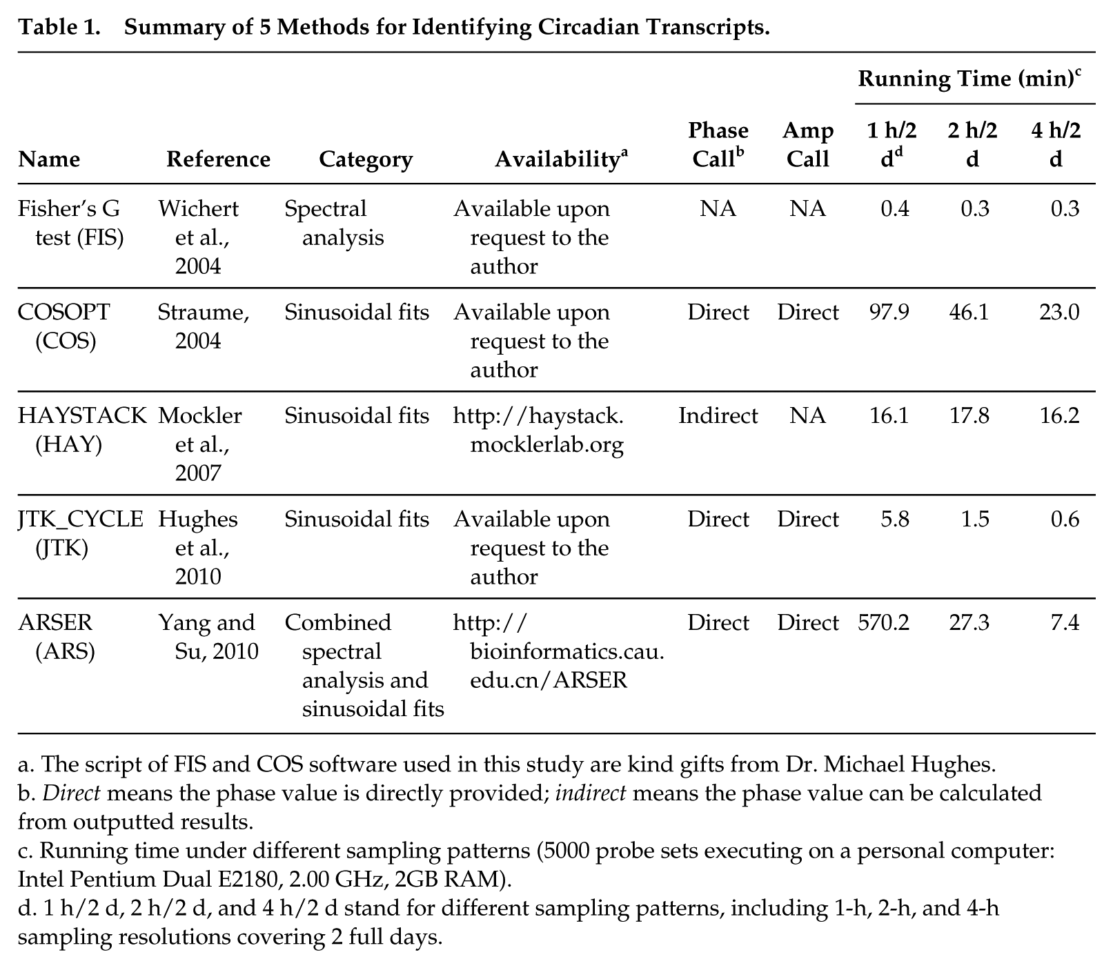
The script of FIS and COS software used in this study are kind gifts from Dr. Michael Hughes.

b.

Direct means the phase value is directly provided; indirect means the phase value can be calculated from outputted results.

c.

Running time under different sampling patterns (5000 probe sets executing on a personal computer: Intel Pentium Dual E2180, 2.00 GHz, 2GB RAM).

d.

1 h/2 d, 2 h/2 d, and 4 h/2 d stand for different sampling patterns, including 1-h, 2-h, and 4-h sampling resolutions covering 2 full days.

Testing on Simulated Datasets

Sensitivity and specificity

To examine the sensitivity and specificity of 5 methods in distinguishing circadian from noncircadian signals, we use the ROC curve. The AUC represents the power of correctly identifying circadian transcripts. We test the performance of each method in analyzing stationary periodic profiles (cosine, cosine2, cosine peak, sine triangle, and sine square) at different amplitudes (low, median, and high amplitude; Figure 1). As the amplitude varies from low to high, all examined methods tend to present increasingly better power in identifying periodic profiles (Figure 1). For example, the AUC of ARS in identifying cosine2 periodic profiles is 0.792 at the low amplitude, 0.917 at the median amplitude, and 0.960 at the high amplitude, respectively. At the same amplitude level, cosine and triangle curves are relatively easier to be identified (Figure 1) by different methods compared with the cosine2 curve.

Figure 1.

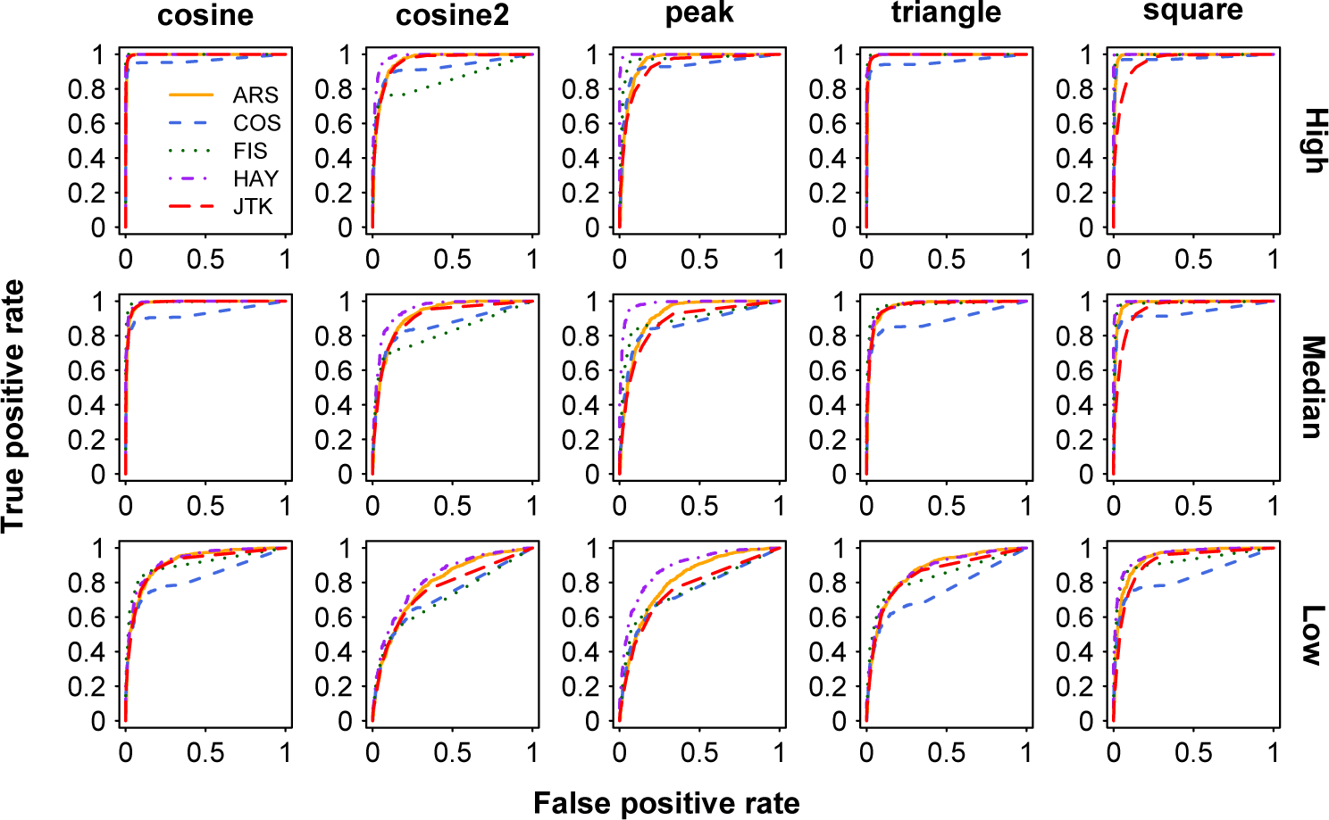
ROC curves for identification of stationary periodic profiles at 3 levels of amplitudes. The shapes of 5 periodic profiles are shown in columns and 3 levels of amplitudes are in rows. High, median, and low amplitude represent amplitude normally distributed between 1 and 2, between 2 and 3, and between 3 and 5, respectively. The SD of noise is 1, and sampling pattern of each periodic profile is 4 h/2 days. Color available in the online version of this article.

In addition, we use different sampling patterns and examine their influence on the power of different methods when fixing the amplitude and noise level (see Materials and Methods). Within the same time window length (2 full days), each method is able to identify any shape of periodic profiles at 1-h and 2-h sampling resolutions (all AUCs are larger than 0.933) by comparison with the 4-h sampling resolution. At a given sampling frequency (e.g., 2-h sampling resolution), all examined methods yield increasing performance in identifying periodic signals when the sampling time window increases from 1 day to 2 days. For example, the AUC of JTK for identifying triangle periodic profiles is 0.936 under 2 h/1 day and 0.997 under 2 h/2 days, respectively. As demonstrated above, more samples generated by increasing sampling frequency or lengthening sampling time window are beneficial for each method in correctly identifying rhythmic signals, which is consistent with previous findings (Deckard et al., 2013). We further test whether higher sampling frequency and longer sampling time window have different influences on each method. When the number of samples is fixed at 12, we use 2 sampling patterns for this test: 2 h/1 day and 4 h/2 days. We find that HAY and JTK tend to perform a little better (a little larger mean value of AUCs; except the cosine2 curve) at 2 h/1 day than at 4 h/2 days, whereas ARS, COS, and FIS yield obviously worse performances at 2 h/1 day than at 4 h/2 days (Figure 2). When identifying triangle periodic profiles under the 4 h/2 days and 2 h/1 day sampling patterns, taking HAY and COS, for example, the AUC of HAY increases from 0.949 to 0.956, while the AUC of COS decreases from 0.856 to 0.649. In addition to stationary periodic profiles, we also examine the higher frequency or longer sampling time window preference on nonstationary periodic profiles and obtain similar results (Suppl. Fig. S2).

Figure 2.

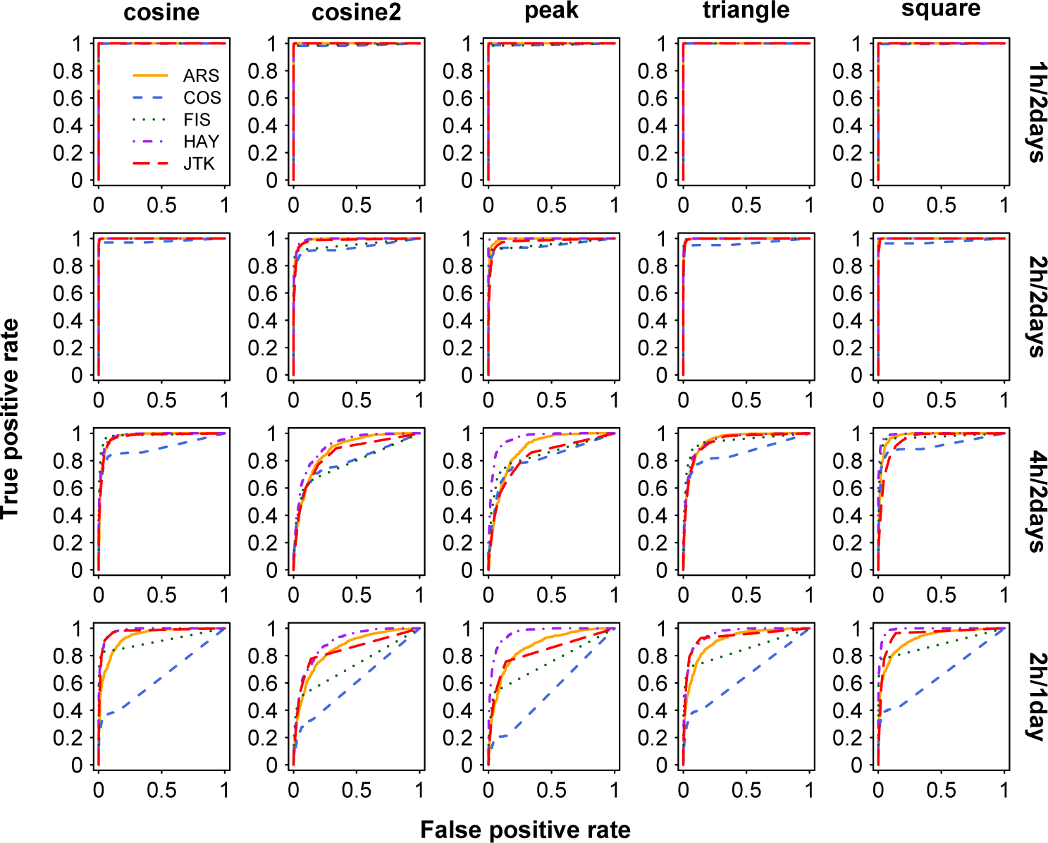
ROC curves for identification of stationary periodic profiles under 4 sampling patterns. The shapes of 5 periodic profiles are shown in columns and 4 sampling patterns are in rows. The amplitude of each periodic profile is 2, and the SD of noise is 1. Color available in the online version of this article.

Circadian phase and amplitude

Since circadian genes with similar phase may be operated under a common regulatory mechanism, accurate calculation of circadian phase is vital for understanding the circadian system and exploring potential mechanisms. We use the delta phase (dPHA) to examine the accuracy of each method in phase prediction with various sampling patterns. For a given time window length (2 full days) and amplitude level (amplitude = 2), all tested methods give more accurate phases (lower means of the absolute values of dPHA) under the 1 h/2 days and 2 h/2 days sampling pattern than under the 4 h/2 days sampling pattern (Figure 3), for nearly all shapes of periodic profiles (except HAY in analyzing square periodic profiles). At the same sampling frequency (2-h sampling resolution), all tested methods exhibit better performance in phase prediction (Figure 3) when increasing the sampling time window length (except JTK in analyzing peak and cosine2 periodic profiles) from 1 day to 2 days. When the number of samples (4 h/2 days and 2 h/1 day sampling pattern) is fixed (Figure 3), JTK achieves more accurate circadian phases of periodic profiles at higher sampling frequency (2 h/1 day), whereas ARS and COS perform better at the longer sampling time window (4 h/2 days). For example, considering triangle periodic profiles, the means of the absolute values of dPHA under the 4 h/2 days and 2 h/1 day sampling patterns are 1.31 and 0.97 for JTK, 1.08 and 1.31 for ARS, and 1.03 and 1.15 for COS, respectively. It is noted that all tested methods are not good (means of the absolute values of dPHA are larger than 1.10) at predicting phases of cosine2 periodic profiles and always underestimate them (more than 65% of medians of dPHA are below 0). Intriguingly, JTK usually overestimates circadian phase for noncosine2 periodic profiles (more than 56% of medians of dPHA are above 0).

Figure 3.

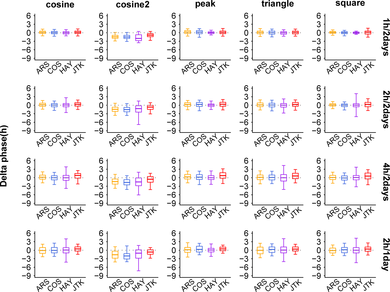
Evaluation of 5 methods at predicting phase. The shapes of 5 periodic profiles are shown in columns and 4 sampling patterns are in rows. The boxes depict data between the 25th and 75th percentiles with central horizontal lines representing the median values and with whiskers showing the 5th and 95th percentiles. Gray dashed line indicates that delta phase (dPHA, predicted phase minus expected phase) is zero (indicating correct prediction). In calculating dPHA, we use only those periodic profiles with significant p-values (p < 0.05). Color available in the online version of this article.

Regarding amplitude estimation, we use delta amplitude (dAMP) based on simulated datasets containing 5 stationary curves with varying amplitude levels under the same sampling pattern (4 h/2 days). With an increase of amplitudes, the performance of each method becomes worse at amplitude estimation, as indicated by larger dAMP (except COS in analyzing cosine periodic profiles; Suppl. Fig. S3). For a specific amplitude level, amplitudes of cosine periodic profiles are relatively easier to estimate (lower means of the absolute values of dAMP) by different methods compared with square profiles (Suppl. Fig. S3).

Testing on Empirical Datasets

We apply all 5 methods in empirical datasets, investigate their overlapped circadian transcripts after correcting the FDR, and evaluate their performance in the identification of circadian genes. In addition, we specifically study the top 20 circadian benchmark genes identified by each method and explore their detailed expression profiles.

Overlapped circadian probes

The number of circadian transcripts identified by different methods varies greatly (FDR < 0.05; Suppl. Fig. S4). Specifically, HAY and FIS derive a total of 40,020 and 5443 circadian transcripts from the 1 h/2 days empirical dataset, respectively. Higher frequency of temporal sampling (within the same time window length) is beneficial in reducing the controversy of circadian transcripts identified by different methods. There are 3759 mutual circadian transcripts (9.4% of all circadian transcripts) identified by 5 methods in the 1 h/2 days empirical dataset (Figure 4A). Interestingly, the same count is also obtained by 4 non-HAY methods (Figure 4B), which accounts for about 36.4% among all circadian transcripts identified by them. Likewise, in the 2 h/2 days empirical dataset, all 5 methods and 4 non-HAY methods yield 507 mutual circadian transcripts that account for about 1.4% and 10.2% of all circadian transcripts identified by 5 and 4 methods, respectively (Figure 4C and 4D).

Figure 4.

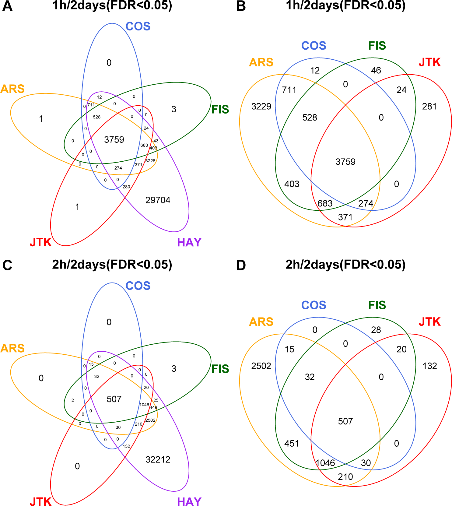
Illustration of overlapped circadian transcripts identified by different methods. Venn diagrams display the relationship of identified circadian transcripts under the 1 h/2 days sampling pattern among 5 (A) or 4 (B) methods and under the 2 h/2 days sampling pattern among 5 (C) or 4 (D) methods at FDR < 0.05. Color available in the online version of this article.

Performance of identifying circadian genes

We further evaluate their performance at identifying circadian genes from datasets under different sampling patterns based on 104 liver circadian and 113 noncircadian benchmark genes (Suppl. Table S4). To synchronously take into account circadian and noncircadian benchmark genes identified by each method at a given FDR level, we use the MCC-like value. MCC-like value ranges from −1 to 1, with larger MCC-like values representing better performance.

Consistent with the results based on simulation datasets, more samples obtained by increasing sampling frequency or lengthening the sampling time window (Figure 5 and Suppl. Fig. S5) are advantageous for each method. For example, COS, FIS, and JTK show better performance (higher means of MCC-like values; Figure 5A and 5B) in analyzing empirical datasets under the 1 h/2 days than the 2 h/2 days sampling patterns at FDR < 0.05. Under the same threshold, HAY presents worse performance, as indicated by much lower mean MCC-like value, than COS, FIS, and JTK (Figure 5A and 5B), and ARS exhibits worse performance (lower means of MCC-like values; Figure 5A and 5B) in analyzing empirical datasets under the 1 h/2 days than the 2 h/2 days sampling pattern. The worse performances of ARS and HAY are presumably due to inclusion of more noncircadian benchmark genes identified by them. At a more stringent threshold (FDR < 5e-5), the MCC-like value of HAY is high, and ARS shows higher MCC-like values in analyzing the empirical dataset under the 1 h/2 days than the 2 h/2 days sampling pattern (Suppl. Fig. S5A and S5B), which is comparable with the results by the rest of the 3 methods at FDR < 0.05. With a fixed number of total samples (12 in count), FIS and JTK exhibit better performance at a higher sampling frequency, as testified by larger MCC-like values in the 2 h/1 day than in the 4 h/2 days empirical dataset (Figure 5C and 5D). ARS shows better performance with a longer sampling time window (Figure 5C and 5D). Considering that HAY and COS always show high false-positive and false-negative rates, respectively, when a stricter FDR threshold (FDR < 0.001; Suppl. Fig. S5C and S5D) for HAY and a looser FDR threshold for COS (FDR < 0.5; Suppl. Fig. S5E and S5F) are used to redo this analysis, we find that HAY and COS prefer higher sampling frequency and the longer sampling time window, respectively. The higher sampling frequency or longer sampling time window preference of ARS, COS, HAY, and JTK is consistent with the result obtained from simulated datasets, while FIS shows results opposite to those based on simulated datasets (discussed below). As noted, MCC-like values of 5 methods at the same FDR level vary dramatically, and thus one should be cautious in selecting a specific significance level when comparing circadian genes from different methods.

Figure 5.

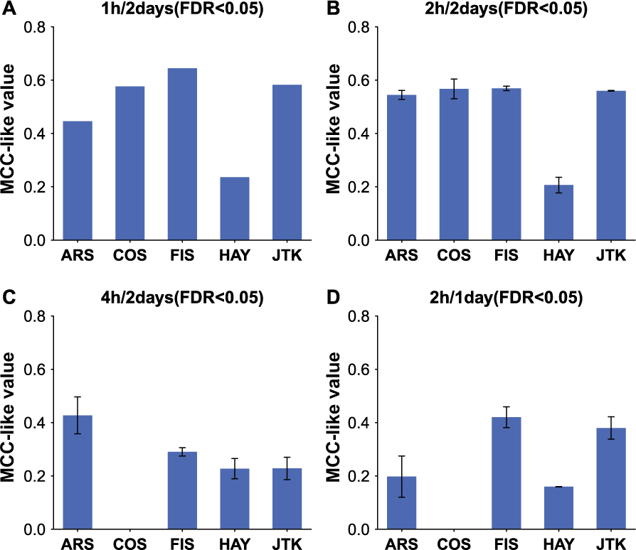
Estimating the performance of multiple methods at identifying circadian genes. The performance of each method in identifying circadian genes from empirical datasets under the 1 h/2 days (A), 2 h/2 days (B), 4 h/2 days (C), and 2 h/1 day (D) sampling patterns is measured by MCC-like value at FDR < 0.05. A larger MCC-like value indicates better performance. If multiple empirical datasets are under the same sampling pattern, we show the average MCC-like value with standard deviation.

Preferable periodic curve shapes

We investigate expression profiles of top 20 circadian benchmark genes identified by 5 methods from the 1 h/2 days empirical dataset (Figure 6). All circadian benchmark genes are ordered according to p-values of their representative circadian probe sets. In cases where several circadian genes receive the same score, we order them by their RefSeq loci ID. Among the top 20 identified circadian benchmark genes at FDR < 0.05, 6 genes (Elovl3, Insig2, Nampt, Nr1d2, Rorc, and Tef) are detected in common by all methods (although p-values given by different methods may differ from each other). Agreeing with a previous report (Deckard et al., 2013), one method always gives lower p-values for its preferable periodic curve shape, which we can see from expression profiles of method-specifically identified circadian benchmark genes. Shapes that are very similar to cosine peak curves (Fkbp5, Lpin1, Usp2, and Ccrn41) appear in JTK-specifically identified top 20 circadian benchmark genes. These results conform well to results obtained from simulated datasets—that is, JTK gives lower p-values to peak periodic profiles (Suppl. Fig. S6). Additionally, among the top 20 circadian benchmark genes, we find that expression profiles of circadian genes (Hlf, Acot4, Acot3, and Ppara) specially identified by COS appear to be noisier than those only identified by other methods.

Figure 6.

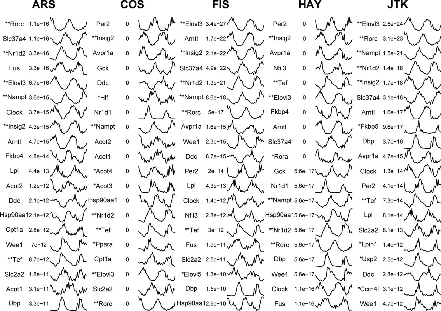
Expression profiles of top 20 circadian benchmark genes identified by each method. Methods are shown in 5 main columns, with each column divided into 3 subcolumns showing gene symbol, p-value, and expression profile, respectively. Each expression profile is normalized by its median expression value among all time points. *Method-specific identified circadian benchmark genes. **Common circadian benchmark genes identified by 5 methods.

Discussion

Here we explored the characteristics of 5 popular methods by evaluating their performance in identifying circadian signals based on both simulated and empirical datasets. FIS is fastest in terms of running time, which may be at the cost of lacking a phase call (Wichert et al., 2004). Among the rest of the 4 methods that provide a phase call in a direct or indirect manner, JTK is the fastest, probably due to high efficiency of statistics calculation in its design (Hughes et al., 2010) and the small number (no more than 216) of rhythmic models used for identifying circadian transcripts. HAY employs relatively small and equal numbers (360 in count) of periodic models, which may result in its running time being insensitive to sample numbers. Unlike JTK and HAY, COS incorporates a very large number (101,000 in count) of periodic models (Harmer et al., 2000; Straume, 2004), accordingly provoking the sensitivity of running time to sample numbers (about 2-fold difference in running time between 1-h and 2-h sampling resolution over 2 full days; Table 1). ARS takes much more time (about 20-fold larger; Table 1) in analyzing 5000 transcripts under the 1 h/2 days than the 2 h/2 days sampling pattern, which is presumably due to nonlinear increment of peaks in the spectrum of transcripts from the 2-h to 1-h sampling resolution.

In addition to running time, we also investigated characteristics of 5 methods in analyzing periodic profiles varying in amplitudes and sampling patterns. It should be mentioned that low, median, and high amplitudes in this study are relative to a fixed noise level (SD = 1). When the noise level is changed, the values of low, median, and high amplitudes will change proportionally. We found that each method shows equal AUC when both amplitude of periodic profiles and SD of noise are set to 1 or 2 (data not shown). Sampling pattern is fundamentally determined by 2 factors: sampling frequency and sampling time window length. When fixing one factor, increasing the other one will yield more samples. Consistent with previous results (Deckard et al., 2013), sufficient samples are beneficial for improving the performance of each method in identifying periodic signals. Interestingly, under the fixed number of total samples, higher sampling frequency is more important for HAY and JTK, while the longer sampling time window is more crucial for ARS and COS, which are consistently observed from both simulated and empirical datasets. The specific preference of each method on high sampling frequency and long sampling time window may be caused by the difference of algorithm design in detecting rhythmic signals. In detail, ARS uses autoregressive spectral analysis in detecting periodic components from time-series profiles. Time points covering more cycles may be more crucial for improving the performance of autoregressive spectral analysis.

FIS prefers the longer sampling time window in simulated datasets but shows higher sampling frequency preference in empirical datasets. This inconsistency may be caused by a period length filtering step in applying FIS. Period length filtering has significant influence on analyzing periodic profiles at lower amplitudes. For example, 972 peak periodic profiles (total of 1000 with the 4 h/2 days sampling pattern) at high amplitudes remained, whereas only 649 at low amplitudes remained after the period length filtering step (without setting a significance threshold). Therefore, this step may have different influences on identifying simulated periodic profiles at median amplitudes and circadian benchmark genes (usually at significantly high amplitudes), which lead to the inconsistent results between simulated and empirical datasets.

All methods can estimate period length of identified circadian transcripts, whereas not all can present the other 2 circadian parameters—circadian phase and amplitude. Although FIS does not provide circadian phase, it should be mentioned that it does not mean that methods applying Fourier analysis cannot calculate circadian phase. According to our results (Figure 3 and Supp. Fig. S3), each method can hardly estimate the correct circadian phase and amplitude. The estimation of these circadian parameters may be a side effect in the algorithm design of studied methods. Therefore, attention should be paid to using the circadian phase and amplitude presented by each method in circadian transcriptome studies.

In a typical circadian transcriptome study, the p-value or FDR threshold, conventionally set at 0.05, is often used for selecting circadian genes. HAY and COS always identify more and less circadian transcripts than others (Figure 4 and Suppl. Fig. S4), which may be associated with their higher false-positive and false-negative rates at a given FDR threshold. These results imply that attention should be paid when applying the same threshold for different methods in selecting circadian genes, especially for HAY and COS. Furthermore, as previously reported (Deckard et al., 2013), each method has its own defined rhythmic signals. Thus, they may show preference for a specific shape of periodic profiles, suggesting that it is beneficial to determine periodic patterns of interest before selecting the optimal one from multiple methods.

Although our comparative study offers potentially important insights on selecting an appropriate method for identifying circadian genes, there are limitations in our work. First, due to restricted literatures, the circadian and noncircadian benchmark genes are relatively limited. Second, the simulation conducted here is not comprehensive; expression patterns of simulated periodic transcripts may be too simple compared with expression patterns of real circadian genes, and thus we cannot exclude the possibility of introducing bias arising from simulation. Third, we compared the performance of 5 methods in genome-widely identifying circadian genes at the organism level and did not evaluate them in identifying a smaller group of circadian genes at the cell line level.

To summarize, in a circadian study, it is advisable to increase the number of total samples, which, as demonstrated here, is not only helpful at accurately identifying circadian transcripts (Figures 2, 4, and 5) but also beneficial in correctly estimating circadian phase (Figure 3). For any dataset with a given sampling pattern, it is of crucial significance to select an optimal one from different methods according to their diverse characteristics. Moreover, our results suggest that caution should be paid in setting a common threshold for each method in selecting circadian genes, especially when applying 2 or more methods to the same dataset. We also suggest that future developments of methods for identifying circadian genes include advancing computational efficiency, adding a direct phase call step, using point estimation in measuring circadian parameters, and improving statistical models, which may potentially provide more important insights on the circadian system as well as on its associated underlying mechanisms.