Wavelet-Based Time Series Analysis of Circadian Rhythms

Abstract

Analysis of circadian oscillations that exhibit variability in period or amplitude can be accomplished through wavelet transforms. Wavelet-based methods can also be used quite effectively to remove trend and noise from time series and to assess the strength of rhythms in different frequency bands, for example, ultradian versus circadian components in an activity record. In this article, we describe how to apply discrete and continuous wavelet transforms to time series of circadian rhythms, illustrated with novel analyses of 2 case studies involving mouse wheel-running activity and oscillations in PER2::LUC bioluminescence from SCN explants.

Circadian rhythms are characterized by approximately 24-hour cycles of some observable variables such as locomotor activity or clock gene expression. The period of some rhythms can be quite precise, for example, the cyanobacteria Synechococcus elongatus (Mihalcescu et al., 2004), but circadian oscillations can also exhibit considerable variability in period and amplitude over time. Here, we describe cases where period and/or amplitude vary over time and for which wavelet analysis provides a means to describe aspects of the data that cannot be obtained through more traditional methods. Wavelet transforms can be applied to directly measure period and amplitude as they vary over time in an activity record or bioluminescence time series. Alternatively, they can be used to eliminate noise and trend from time series to facilitate estimation of phase markers such as peak time. Wavelet methods can also be used to assess the strength of signal components lying in different frequency bands, for example, ultradian versus circadian components of an activity record. In this article, we provide a full description of this new approach with information that will allow researchers with similar requirements to apply wavelet analysis to their data.

Wavelet analysis has been previously applied to the field of chronobiology in a few instances, for example, to study ultradian activity rhythms (Poon et al., 1997; Chan et al., 2000) and to decompose Drosophila mating songs (Dowse, 2009). Price et al. (2008) and Baggs et al. (2009) used continuous wavelet transforms with ridges to analyze cell luminescence data. Etchegaray et al. (2010) used a similar wavelet analysis to analyze regulation of circadian period length by casein kinase 1δ in mouse SCN neurons. Meeker et al. (2011) applied wavelet analysis to analyze period instability in SCN neurons. Here, we provide further examples to demonstrate cases where this approach is helpful, and we provide background and methods directed toward the circadian researcher new to the application of wavelet analysis. Technical material is separated from the main text into 4 boxes: Box 1 describes nonstationary signals, Box 2 briefly reviews Fourier analysis of time series, Box 3 defines the discrete wavelet transform, and Box 4 explains the analytic wavelet transform. After a basic introduction describing wavelet analysis, we present 2 case studies to illustrate how these methods go beyond more traditional methods of analysis.

Box 1.

Nonstationary Signals

Sinusoids are the canonical periodic signals. For example, the signal

$$x(t)=A\cos \left(\frac{2\pi }{\tau }(t-t_0)\right)$$

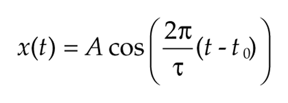
oscillates with frequency 2π/τ, equivalent to a period of τ, has amplitude A, and peaks at time t₀ (and every τ time units thereafter). In contrast, the period and amplitude of nonstationary signals vary over time. An oscillatory signal that may vary in amplitude and frequency over time has generic form

$$x(t)=a(t)\cos \theta (t).$$

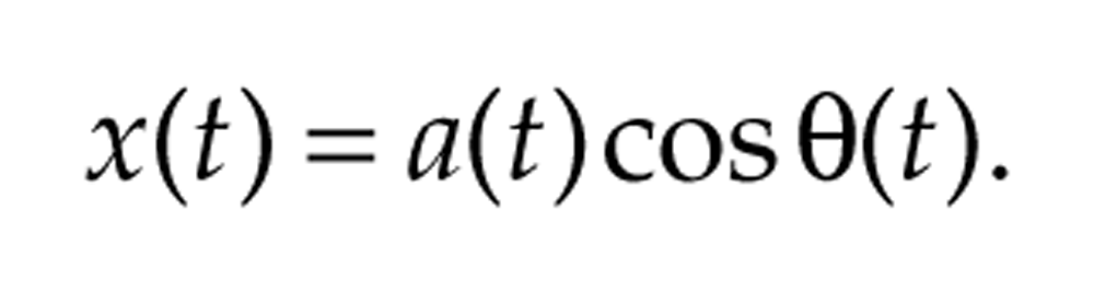
For instance, the frequency of the signal

$$x(t)=A\cos \left(\frac{2\pi }{{\tau }_c}t+\frac{{\tau }_m\Delta f}{2\pi }\sin \left(\frac{2\pi }{{\tau }_m}t\right)\right)$$

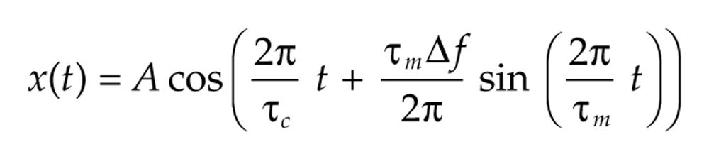
varies around a central frequency of 2π/τ _c by ±Δf every τ _m time units. The instantaneous frequency of such signals is the derivative θ′(t) of the phase function. In the case of a fixed frequency signal with θ(t) = 2πt/τ, the derivative is 2π/τ, and so the instantaneous frequency agrees with the usual definition of frequency. We can also vary the amplitude a(t) over time, for example,

$$x(t)=\left(A+\Delta A\cos \left(\frac{2\pi }{{\tau }_m}t\right)\right)\cos \left(\frac{2\pi }{t}\left(t-t_0\right)\right).$$

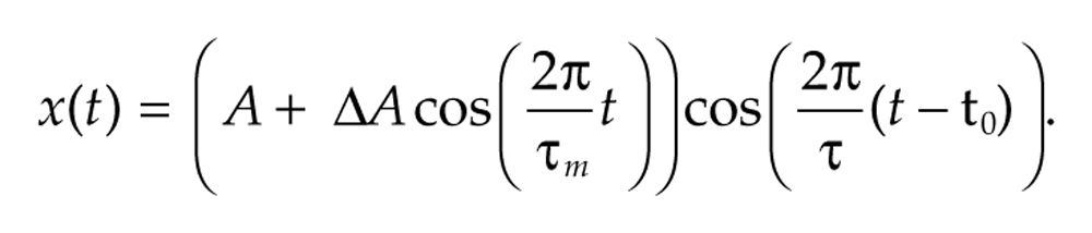
See chapter 4 of Mallat (2009) for more details.

Box 2.

The Discrete Fourier Transform (DFT)

A central objective of discrete Fourier and wavelet analysis is to express a signal as a sum of waveforms. Fourier analysis utilizes cosines and sines of different frequencies, conveniently expressed mathematically as e²π ^ikt = cos2πkt + isin2πkt, where $i=\sqrt{-1}$ . Suppose a signal x = {x_k} is created by measuring some quantity every Δt hours for a total of N measurements labeled x₀, x₁, . . ., x _{N – 1}, so that x_n corresponds to time t = nΔt/N. The DFT coefficient X_k of x is defined to be

$${\text{X}}_k={\displaystyle \sum _{n=0}^{N-1}{x}_n{e}^{-2\pi ikn/N}.}$$

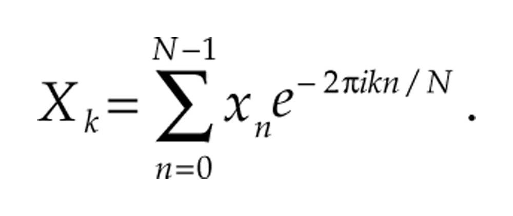
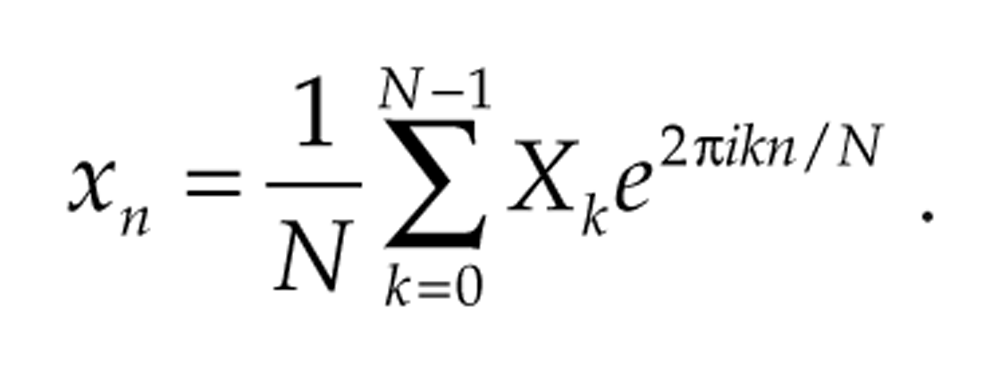
The fast Fourier transform (FFT) is a very efficient algorithm used to compute the DFT of signals for which N is a power of 2, but the DFT may be applied to signals of any length N. The adjusted Fourier coefficient X_k/N is the amplitude associated with component e²π ^ikt ; that is, the DFT allows us to decompose the original signal into a sum of sinusoidal components:

$$x_n=\frac{1}{N}{\displaystyle \sum _{k=0}^{N-1}{X}_k{e}^{2\pi ikn/N}.}$$

The sinusoidal functions of Fourier analysis are excellent for determining what frequencies are present in a signal, but because sinusoids oscillate at a fixed frequency for all time, they cannot be used to assess how the period of a signal varies over time. Figure 1 illustrates these ideas. For more details, see chapter 3 of Mallat (2009).

Box 3.

The Discrete Wavelet Transform (DWT)

Wavelet transforms typically involve waveforms that have finite support, that is, are nonzero on a finite length interval, in contrast to cosines and sines that oscillate for all time. Whereas the DFT decomposes a signal x into a sum of sinusoids at particular frequencies, the DWT splits x into components called wavelet details and smooths that are associated with different frequency bands. This is accomplished by repeatedly applying a high-pass wavelet filter (HPF) to generate wavelet coefficients W_j,k and a low-pass scaling filter (LPF) to generate scaling coefficients V_j,k. See Figure 2 for graphs of the wavelet and scaling filters used in this article.

The wavelet coefficients W_j,k yield the level j wavelet detail D_j, and the scaling coefficients V_j,k yield the level j wavelet smooth S_j, via application of the inverse DWT. The original signal x is the sum of the wavelet details D₁, . . ., D_J plus the final wavelet smooth S_J, where J is the number of levels computed. Figure 2 illustrates this process for J = 3. The wavelet detail D_j corresponds to a frequency band with period range 2 ^j Δt to 2 ^j +¹Δt time units, where the signal x was created by sampling every Δt time units. Hence, each level is associated with a scale twice as long as the previous level’s. The wavelet smooth S_J is obtained by repeated smoothing via the LPF and so forms the trend of the signal. Together, the wavelet details and smooth form a multiresolution analysis (MRA) of the signal, exemplified in Supplementary Figure S2 for bioluminescent signals. We use a translation-invariant DWT (also known as a stationary or maximal overlap DWT) that does not downsample like the regular form of the DWT. For more information, see Percival and Walden (2000).

Box 4.

The Analytic Wavelet Transform (AWT)

In contrast to the DWT that uses a pair of real-valued filters, the AWT involves a complex-valued wavelet function ψ(t) that corresponds to a frequency band determined by its DFT, as illustrated in Figure 3 for the Morse wavelet function. The AWT of a signal x(t) at time t and scale s is defined to be

$$\text{W}(t,s)={\displaystyle \underset{-\infty }{\overset{\infty }{\int }}\frac{1}{s}}{\psi }^{*}\left(\frac{u-t}{s}\right)x(u)du,$$

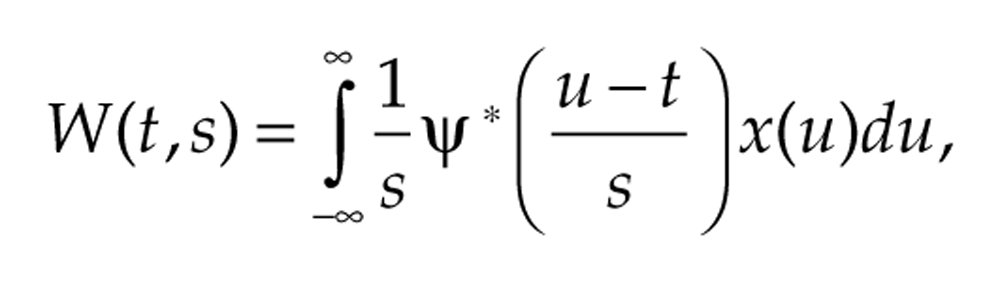
where the asterisk denotes the complex conjugate (reverses the sign of the imaginary part). Essentially, the wavelet transform correlates the given signal x(t) with wavelet functions that have been translated to be centered at time t and scaled by a factor s (thereby altering the period). At a given time t, we identify the period of the signal by finding the scale that maximizes the wavelet transform (hence, the correlation) between the signal and the scaled wavelet. This is the idea behind the wavelet ridge, which estimates the instantaneous frequency and amplitude of the signal at each time point. Wavelet ridge curves run along local maxima with respect to s (for each fixed t) of the absolute value of the AWT and thereby indicate the signal’s instantaneous frequency and analytic amplitude at each time point, as shown in Supplementary Figure S5 for 2 examples. We use bandpass normalization, as described in Lilly and Olhede (2009), so that |W(t, s)| can be directly interpreted as amplitude. The transform essentially finds the correlation between the signal and the wavelet function, and the ridge curve identifies the waveforms that have the greatest correlation with the signal. The scale s can be interpreted as frequency via ω = ϕ/s or as period via τ = 2πs/ϕ, where ϕ is the mean frequency of the wavelet function ψ(t). The AWT also yields phase information because each complex number z = reⁱθ encodes both amplitude r and phase angle θ.

Another way to understand what the AWT does is to examine the transform’s action in the frequency domain, in the same way we examine how filtering works in Supplementary Figure S1. We can reformulate the definition of W(t, s) to work in the frequency domain rather than in the time domain:

$$\text{W}(t,s)=\frac{1}{2\pi }{\displaystyle \underset{-\infty }{\overset{\infty }{\int }}\frac{1}{s}}{\psi }^{*}(s\omega )\text{X}(\omega )e^{i\omega t}d\omega$$

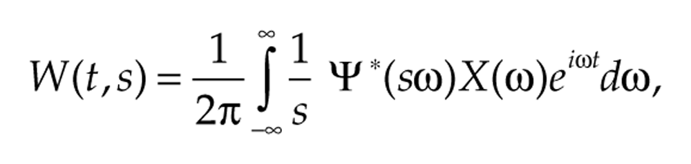
where X(ω) and Ψ(ω) are the Fourier transforms of x(t) and ψ(t), respectively. This says that the AWT is in effect multiplying the signal’s frequency spectrum by the wavelet function’s Fourier transform Ψ (Fig. 3). Changing s shifts Ψ(sω) along the frequency axis, and the ridge location corresponds to the value of s that maximally matches Ψ(sω) with the signal’s frequency profile X(ω). See Lilly and Olhede (2010), Selesnick et al. (2005), and chapter 4 of Mallat (2009) for further information about the AWT.

Introduction to Wavelet Analysis

Accurate determination of period length is critical for most circadian studies. Common techniques including the Fourier periodogram, sine wave fitting, maximum entropy spectral analysis (MESA), and autocorrelation-based methods assume that the intrinsic period and amplitude do not change over time, as is true for stationary time series. These methods yield good results for most experimental data when applied appropriately, with the best choice of method depending on the characteristics of the particular time series. The resolution of the Fourier periodogram, which is essentially the discrete Fourier transform (DFT), depends on the number of cycles contained in the data and so requires a relatively long record (typically at least 10 cycles). Autocorrelation yields a period estimate with resolution that depends on the sampling interval and is best applied to records with at least 4 cycles and a short sampling interval. MESA has finer resolution than the Fourier periodogram and works reasonably well even for short, noisy time series as long as the period and amplitude do not vary significantly over time. Unlike the previous 3 methods, sine wave fitting is not restricted to a grid of periods and can be applied to short time series (3 or more cycles for good results), but it is more sensitive to variations in period and amplitude. See Levine et al. (2002) and Dowse (2009) for further details on these commonly used methods for circadian data.

While performing well in many circumstances, traditional methods can be unreliable when applied to data with significant variation in amplitude and period across cycles, that is, nonstationary time series (Box 1), and none of them measures how the period may be changing over time within a time series. Because circadian data are often nonstationary (Refinetti, 2004), these traditional methods may be inadequate in some cases, and wavelet-based approaches may prove more effective for determining period length as well as offering a means of measuring variability in period and amplitude within a time series.

Wavelet analysis, similar to Fourier analysis, attempts to express a signal as a sum of component waveforms. Whereas the waveforms in Fourier analysis are sines and cosines of a set of fixed frequencies (Box 2 and Fig. 1), wavelet transforms allow us to decompose a signal in a more flexible manner. In addition to being the method of choice for analyzing nonstationary time series, wavelet analysis has some advantages over traditional methods; for example, wavelet methods do not require removal of noise or trend to accurately measure period. In fact, the discrete wavelet transform (DWT) can itself be a very effective tool to remove trend and noise from a time series by focusing on a desired frequency band, thereby facilitating clear and accurate identification of phase markers such as peaks. The DWT decomposes a time series into components corresponding to different frequency bands in a time-localized manner (Box 3, Fig. 2, and Suppl. Fig. S2), thereby isolating the circadian component to effectively remove trend and noise (Suppl. Fig. S3) as well as partitioning the variance of a time series according to the frequency band (Suppl. Fig. S4). In contrast, a type of complex-valued continuous wavelet transform called the analytic wavelet transform (AWT) directly measures period and amplitude varying over time in a time series (Box 4).

Figure 1.

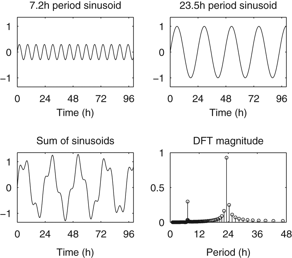
Example of the DFT applied to a simple oscillatory signal. We sum 2 sinusoids with periods of 7.2 hours and 23.5 hours to obtain a signal x. The DFT coefficients’ magnitudes, |X_k|/N, give the amplitude of the sinusoids with frequencies k/N, whose sum will equal the signal x (in this example, N = 1024) (see Box 2). The 2 peak DFT coefficients closely match the periods and amplitudes of the 2 sinusoids, but with “leakage” around the peak frequency due to the DFT frequency corresponding to 23.3 hours, slightly different from the signal’s period of 23.5 hours. The resolution of the DFT depends on the number of cycles present in the signal; if the signal’s peak frequency does not exactly match one of the DFT’s frequencies, the DFT must use a combination of nearby frequencies to match the signal.

Figure 2.

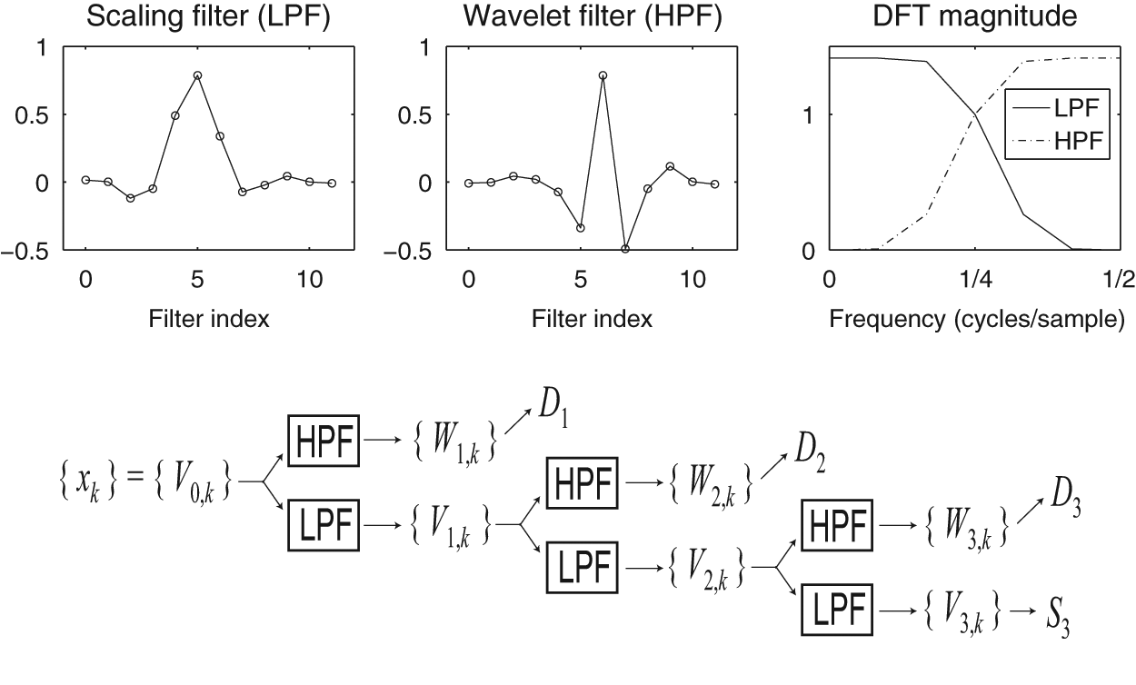
Filters associated with the DWT and the pyramid algorithm used to compute the DWT. Shown here are the Daubechies least-asymmetric wavelet and scaling filters of length 12, along with their DFTs. The wavelet filter is a high-pass filter (HPF) with a DFT magnitude greatest for high frequencies, and the scaling filter is a low-pass filter (LPF) with a DFT magnitude greatest for low frequencies. In the DFT graph, frequency is given in terms of cycles per sample, where the highest possible discernible frequency is one cycle per 2 samples (i.e., signal alternates values at every other time point). The scaling filter acts by multiplying the signal’s DFT by the LPF DFT, thereby retaining only the low-frequency content of the signal. This complements the action of the wavelet filter, which multiplies the signal’s DFT by the HPF DFT, thereby retaining only the high-frequency content. The pair of filters are applied repeatedly as shown in the diagram to yield wavelet coefficients W_j,k (used to generate wavelet detail D_j) and scaling coefficients V_j,k (used to generate wavelet smooth S_j). See Box 3 for further details.

Figure 3.

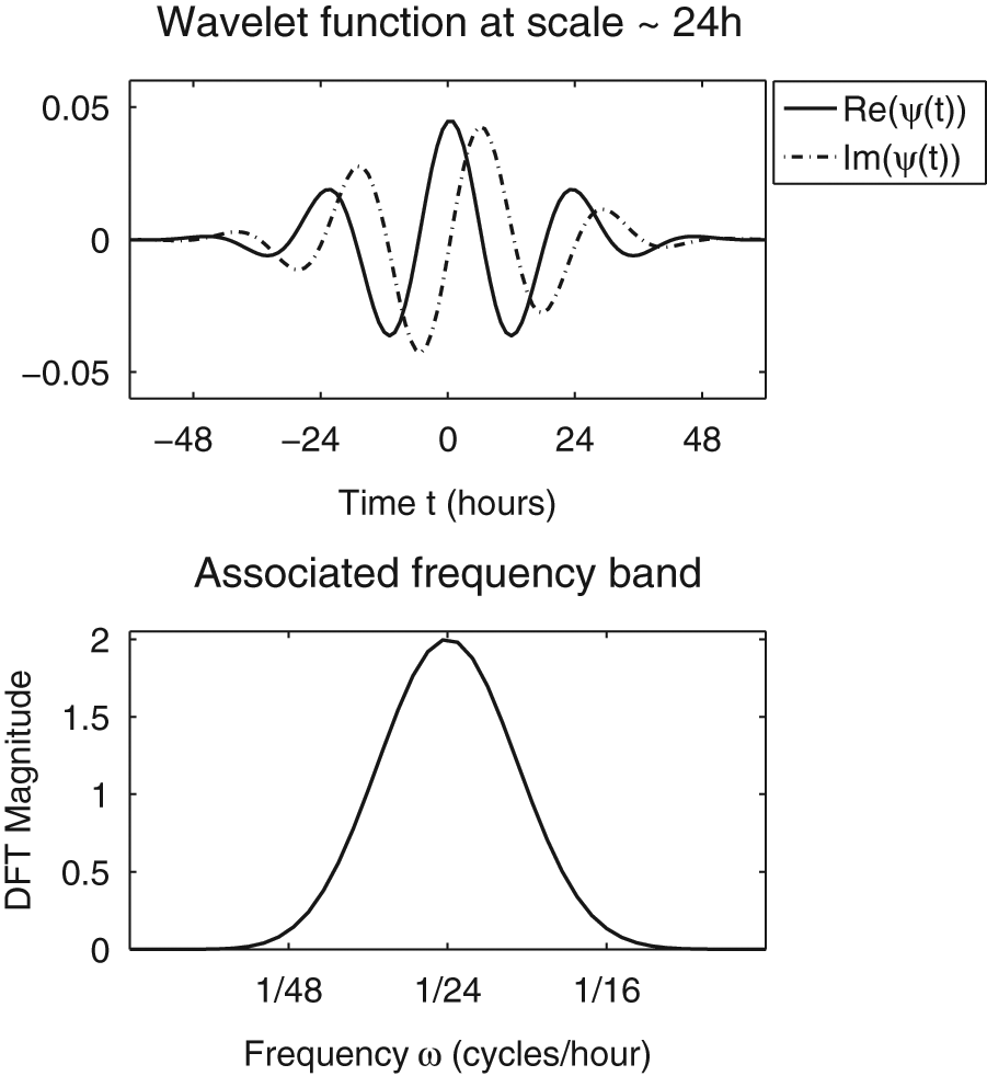
Morse wavelet function (with β = 7 and γ = 3) and its frequency band, used in the analytic wavelet transform in this article. The Morse wavelet function is complex valued, that is, has both real and imaginary parts, allowing it to extract both amplitude and phase information from the signal, which real-valued transforms cannot do. For more details, see Box 4.

Wavelet functions are not periodic, so each wavelet function involves a band of frequencies rather than a single frequency, as illustrated in Figure 3. In switching from Fourier analysis, with its precise frequency determination but lack of time localization, to wavelet analysis, we gain time localization at a cost of some loss of precision in frequency. Because of this “smearing” of frequency content in wavelet functions, we refer to the scale of a wavelet. Each scale corresponds to a frequency band rather than to a single frequency. Large scales correspond to low frequencies (equivalently, long periods) and can be associated with the general trend of a signal, while very small scales correspond to high frequencies and are often associated with high-frequency noise.

The underlying idea behind using wavelet transforms like the AWT to measure period is as follows: Take a wavelet filter (for a discrete transform) or a wavelet function (for a continuous transform), and translate it along the time axis to center it at the time point of interest. Rescaling the wavelet allows us to assess a wide range of frequencies. Compute the correlation between each rescaled wavelet and the time series, and choose the scale that yields the largest correlation. We associate this scale with the mean frequency of the scaled wavelet’s frequency band, thereby allowing us to assign a period to the time series at that time point. The AWT is particularly good for visualizing fluctuations in period as well as in amplitude. The AWT coefficients indicate the correlation between the scaled wavelets and the time series at each time point, often graphed as a heat map with a ridge marking maxima (highest correlation), thereby indicating the period of the time series at each point, as illustrated for simple examples in Supplementary Figure S5. Note that as a consequence of the fact that wavelets are associated with a frequency band rather than a single frequency, the AWT will not distinguish frequencies that are too close relative to the wavelet function’s frequency spread. MESA (Dowse, 2009) can be applied to test whether a signal involves clustered frequencies, as this method can be effective at resolving closely spaced frequencies.

Wavelet methods have application beyond direct period measurement. A multiresolution analysis (MRA) uses the DWT to decompose a signal into components called details associated with different frequency bands and a smooth that can be treated as the trend (Box 3, Fig. 2, and Suppl. Fig. S2). The underlying idea here is to repeatedly apply a wavelet filter to extract details at different scales, while a scaling filter smoothes the signal (analogous to a running average). This method can be used to remove noise and trend to yield a clean signal for examining phase markers such as peaks, for example, in bioluminescence time series. In this manner, the DWT can enhance commonly used methods such as peak picking or sine wave fitting by optimally removing noise and trend from time series, as shown in Supplementary Figure S3. The MRA also partitions the energy of the signal with respect to scale, which can be used to characterize a rhythm or as a rhythmicity criterion by assessing what proportion of the rhythm’s energy lies in a circadian range. Energy in this context equals the variance of the detrended time series; see Supplementary Section S.2 for a rigorous definition and Supplementary Figure S4 for cell data examples. Strong, coherent circadian rhythms are characterized by their energy being concentrated in the frequency band containing the period of the rhythm. This is analogous to how Ko et al. (2010) used the DFT to generate a rhythmicity criterion for SCN neurons by examining the proportion of power in the peak circadian frequency.

Wavelet transforms are powerful tools for assessing rhythmic data, but like the Fourier transform, they must be applied properly to yield valid results. Both Fourier and wavelet methods require time series to be of a minimum length to estimate period with good precision. A particular issue with wavelet transforms and other filtering methods is that of edge effects (distortions in the transformed or filtered signal near its beginning and end). When a wavelet transform is applied at a time t that is near the beginning or end of a time series, the wavelet function or filter runs off the edge, and we must choose a way of extending the time series to fully overlap. Common choices are to pad each end with zeros or with the mean value of the time series. Other choices that can reduce edge effects are to apply periodic boundary conditions (joining the ends to wrap around) or reflection boundary conditions (reflecting about each end) after adjusting the time series to start and end at peaks or troughs. A consequence of artificially extending the time series in any of these ways is that the wavelet transform will be distorted near the edges. It is best to ignore regions exhibiting edge effects, typically at least 1.5 days on each end for frequencies in the circadian range, unless careful measures are taken to minimize boundary distortions. This implies that the data series must cover substantially more than 3 days for wavelet methods to be useful in measuring circadian periods.

We present 2 case studies to illustrate the application of wavelet transforms to circadian data. Case study #1 uses the DWT to characterize the differences between wheel-running rhythms in LD and LL and subsequent effects on SCN PER2::LUC rhythms, while case study #2 applies the AWT to measure period and amplitude modulation in wheel-running activity of a female mouse due to the estrous cycle.

Case Study #1: Wheel Running and Per2::Luc Expression in LD and LL

Background

Constant light disrupts circadian activity rhythms in mice, fragmenting activity bouts, reducing activity levels, and lengthening period (Daan and Pittendrigh, 1976). Ohta et al. (2005) reported that individual SCN neurons in animals housed under constant light continue oscillating but are desynchronized. We expected that constant light would provide a condition under which period and amplitude of the circadian rhythm would vary, so that this would be a case where wavelet analysis would allow greater insight than more traditional methods that assume a stationary signal. We applied wavelet methods to compare activity and bioluminescence records from mPer2^Luc mice under LD 12:12 and LL conditions (see Fig. 4 for representative samples).

Figure 4.

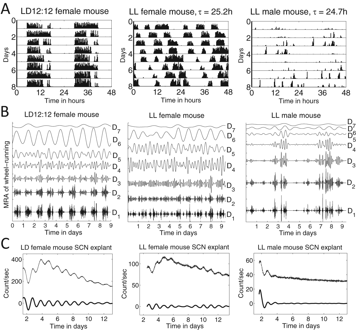
Representative examples of mice under LD 12:12 and LL conditions. (A) Double-plotted wheel-running records with 15-minute bins; periods were computed by MESA after subtracting the mean value. (B) Corresponding MRAs of the wheel-running records in A (smooth S₇ not shown); within each MRA, each detail has mean zero and is plotted with the same axis scaling, so magnitudes can be directly compared. (C) PER2::LUC bioluminescence of SCN explants from the mice whose activity records are shown in A, where graphs display both the raw signal and the signal with noise and trend removed via DWT.

Results

As shown in Figure 5A, activity of mice entrained to LD tends to be greater than activity in LL; the mean activity of male mice under LL is significantly different from that of male mice in LD and of female mice in LD or LL (multiple comparison test, F = 7.5, p < 0.001). To further characterize patterns in wheel running during LD and LL of male and female mice, we used the DWT to partition the energy between ultradian and circadian scales, as described in Supplementary Section S.2 and Supplementary Figure S4. Figure 5B shows the proportion of energy associated with each wavelet detail of mouse wheel-running MRAs (see Fig. 4B for representative samples). Activity in LD has most of its energy in the wavelet detail corresponding to a circadian range of periods (in this example, D₆), while mice in LL display more fragmented activity, with energy distributed among the ultradian scales. Activity under LD 12:12 is characterized by strong consolidation, with energy in the wavelet detail D₆ (corresponding to a circadian range of periods) significantly greater under LD than LL (multiple comparison test, F = 53, p < 0.001). In LL, female mouse activity is distributed among D₃ to D₆, while male mouse activity tends to be fragmented and so predominantly in D₁ to D₃. The period of activity of mice during LL was 25.0 ± 0.3 hours (mean ± standard deviation, MESA; mean period of males and females not significantly different).

Figure 5.

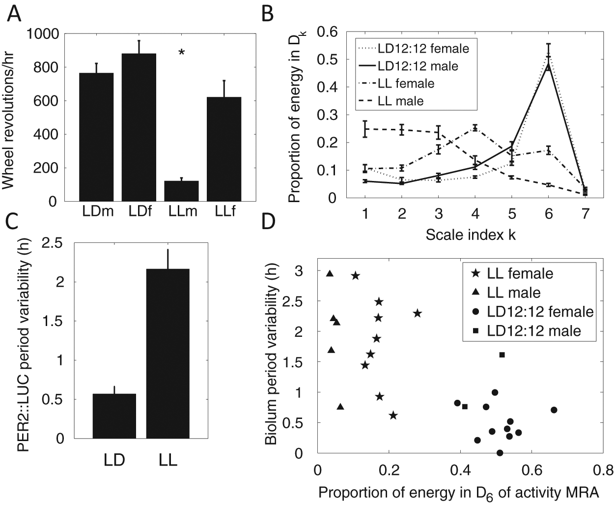
(A) Mean wheel-running activity under LD and LL conditions for male and female mice. Bars show mean ± standard error. (B) Scale-based characterization of wheel-running activity under LD 12:12 and LL for male and female mice (23 LD 12:12 females, 8 LD 12:12 males, 9 LL females, 5 LL males). Error bars indicate mean ± standard error. (C) Period variability of PER2::LUC bioluminescence rhythms in SCN explants, calculated as the standard deviation of 5 consecutive peak-to-peak times following LL and LD conditions. Bars indicate mean ± standard error. (D) Graph showing PER2::LUC period variability versus the proportion of energy lying in the circadian component (wavelet detail D₆) of wheel-running activity. A low proportion of energy in the circadian component of wheel running indicates fragmented activity patterns.

We measured variability in period of PER2::LUC luminescence rhythms of SCN explants by applying a DWT to remove noise and trend (Suppl. Fig. S3), allowing clear discernment of peak times. We then used the standard deviation of 5 consecutive peak-to-peak times as the measure of period variability for each PER2::LUC record. We observed more variability in period following LL than following LD (2-sample t test for unequal variances, t = 5.6, df = 18, p < 0.001) (Fig. 5C). As shown in Figure 5D, there is a significant negative correlation between period variability in the SCN explant PER2::LUC rhythms and the proportion of energy of wheel-running activity in the circadian scale (r = −0.67, p < 0.001). That is, greater period variability in the SCN is associated with more fragmenting of wheel-running activity.

Discussion

The DWT is used here for 2 different purposes: 1) characterizing activity by calculating the energy in each wavelet detail of the wheel-running time series, and 2) removing trend and noise from bioluminescence time series to allow identification of peak times for measuring period variability. Male mice under LL are significantly less active than females and also display greater fragmenting of activity, quantified using wavelet analysis. All mice from LL showed more fragmented rhythms than mice from LD, resulting in most of the energy in activity under LL occurring in the ultradian scales (i.e., higher frequency bands). SCN explants from LL mice also exhibited greater variability in period. The correlation between variability of period in the SCN and fragmenting of locomotor activity suggests that the fragmentation of activity under LL may be partly attributable to destabilized rhythms in the SCN, consistent with the findings of Ohta et al. (2005). While some of these results may be clear by simply looking at the records, the wavelet analysis facilitates an objective quantitative evaluation of, for example, fragmenting of rhythms and variability in period, which is amenable to statistical analysis and can be applied to a wide variety of circadian data.

Case Study #2: Effects of Estrous Cycle on Wheel-Running Records

Background

The estrous cycle can affect the phase, period, and amplitude of rodent locomotor rhythms. Wollnik and Turek (1988) found that the highest amplitude and activity bout length and the shortest circadian period length occurred on the day of estrus in rats for both LD 12:12–entrained and free-running animals. Estradiol shortens the period and advances the phase of wheel running in LD 12:12–entrained ovariectomized golden hamsters (Morin et al., 1977), while progesterone blocks the effects of estradiol on locomotor rhythms (Takahashi and Menaker, 1980). Janik and Janik (2003) found that the resetting of circadian rhythms through novel wheels can induce changes in the estrous cycle of Syrian hamsters. Pilorz et al. (2009) found that wheel-running activity was highest during estrus for wild-type and Per1 mutant female mice but did not vary with the stage of the estrous cycle for Per2 mutants, and Kopp et al. (2006) observed that the second part of the proestrous night was often characterized by increased activity in young female mice. These observed effects of the estrous cycle on locomotor patterns imply that female rodent wheel-running records should be treated as nonstationary time series, and wavelet analysis offers a means of objectively quantifying the variation in period, phase, and amplitude that occurs during the 4- to 5-day estrous cycle.

Results

We examined the wheel-running record of a female mPer2^Luc mouse that was 3 months old at the start of the 20-day record shown in Figure 6A. The animal was well entrained to the LD 12:12 cycle, as indicated by the Fourier periodogram (Fig. 6B) and MESA, both showing strong peaks at 24.0 hours. However, neither the Fourier periodogram nor MESA can reveal time-varying patterns in the period of the mouse’s activity. Therefore, to assess possible fluctuations in period and amplitude over time, we applied an AWT to the wheel-running record shown in Figure 6A to yield the heat map shown in Figure 6C. The wavelet ridge is the best estimate of the instantaneous frequency and amplitude of the signal at each point (Box 4). In Figure 6D, we observe that the wavelet ridge displays a systematic 4- to 5-day variation in period and amplitude, and Supplementary Figure S6 shows the variation in phase angle over time.

Figure 6.

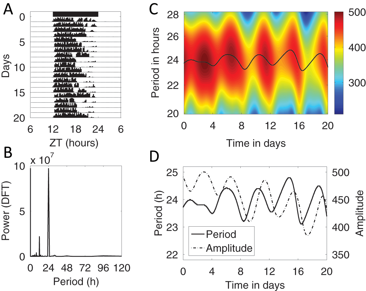
(A) Wheel-running activity of a young female mouse, double plotted with 15-minute bins, ranging from 0 to 1200 revolutions per bin. (B) Fourier periodogram of this wheel-running record. (C) Analytic wavelet transform of the wheel-running record. Color scale indicates amplitude of the activity rhythm (absolute value of AWT coefficients along the ridge, in wheel revolutions per 15-minute bin); double this value to obtain the peak activity level in units of wheel revolutions per 15-minute bin. (D) Replotted wavelet ridge curve showing period over time together with the corresponding amplitude, showing the relationship between the 5-day variation in period and amplitude of wheel running for this mouse. See Supplementary Figure S6 for a plot of the phase angle over time.

While the scalloping of activity can be discerned by the eye in some cases, the AWT provides a means of objectively quantifying the variation over time of period, amplitude, and phase that is associated with the 4- to 5-day estrous cycle. For example, Figure 6C suggests that the amplitude tends to be greatest while the period is growing shorter. We can use the wavelet ridge to more precisely quantify the relationship between period and amplitude variation. Autocorrelation yields a period of 4.1 days for the period and amplitude curves in Figure 6D, with the period rhythm leading the amplitude rhythm by 0.7 days. That is, the shortest period occurs about 0.7 days before the minimum amplitude. Similar patterns can be observed in the examples shown in Supplementary Figure S7.

Discussion

The AWT facilitates visualization as well as quantification of variation in period and amplitude over time. The wavelet ridge curve indicates the period, phase, and amplitude at each time point, thereby providing a means of quantifying changes in these circadian properties over time. In this example, the AWT reveals a 4- to 5-day variation occurring in the amplitude, period, and phase of wheel running that is consistent with the literature concerning the effects of the estrous cycle on activity patterns. The main point of this case study is that the wavelet methods provide an objec-tive way to quantify features of activity records such as recurring changes of period and amplitude. The AWT can also be applied to other types of circadian time series such as bioluminescence rhythms (Price et al., 2008; Baggs et al., 2009; Meeker et al., 2011), and a variety of wavelet functions are available that can be used to detect other types of features, for example, edge detection wavelets that can be applied to detect discontinuities such as activity onsets.

Although both are wavelet transforms, the DWT and AWT are quite different in nature and serve distinct purposes in our analyses. The DWT is real valued and systematically decomposes a signal into details and a smooth, which prove useful for removing noise and trend from a time series (by isolating the circadian component) and for characterizing rhythmicity through partitioning the energy with respect to scale. The effectiveness of the DWT in removing trend and noise can then facilitate other methods such as peak picking to yield period information, but the DWT does not itself directly measure period or amplitude. In contrast, the AWT is complex valued and can directly yield high-resolution measurements of period, phase, and amplitude over time. The difference in these transforms is due to 2 main factors: discrete versus continuous and real valued versus complex valued. The DWT is a discrete transform designed to output components corresponding to fixed frequency bands that exactly add up to the original signal, while the AWT is a continuous transform that scans a range of possible period values in order to determine the best estimate. Real-valued transforms cannot encode both phase and amplitude, as complex-valued transforms can due to the combination of real and imaginary parts (Box 4). Each approach has its advantages and drawbacks. The AWT, for example, tends to underestimate period variations because it essentially averages over several cycles, whereas the DWT/peak-picking method can yield accurate period variability estimates (as used in case study #1). See Selesnick et al. (2005) for an excellent discussion contrasting the DWT with complex-valued wavelet transforms.

Materials and Methods

Experimental Data

Mice (mPer2^Luc, both homozygous and heterozygous) were housed from birth under constant light or under LD 12:12 in standard group housing. At 6 weeks of age, mice were moved to individual cages with running wheels, and activity was monitored for 2 to 3 weeks. Mice were then euthanized with halothane anesthesia, and SCN tissue was cultured as described in Guenthner et al. (2009), with bioluminescence monitored using Lumicycle (Actimetrics, Wilmette, IL). The female mouse (mPer2^Luc heterozygous) analyzed in case study #2 was housed with a running wheel under a LD 12:12 cycle.

Data Analysis

For case study #1, we applied a translation-invariant DWT to wheel-running records with 15-minute bins, using periodic boundary conditions and starting and ending in the middle of rest intervals to minimize edge effects. We chose the Daubechies least-asymmetric filter of length 12 after verifying that longer length filters did not alter the scale energy estimates. We observed that shorter filters reduce edge effects but can yield distorted energy estimates. We also applied this DWT to PER2::LUC bioluminescence time series (10-minute time steps) to extract the circadian component (sum of D₆ and D₇, covering a period range of 11-43 hours) and then used this to determine times of peak luminescence in SCN explants for use in calculating period variability. For case study #2, we applied the AWT using a Morse wavelet function with β = 7 and γ = 3. We chose the Morse wavelet rather than the Morlet wavelet used by Price et al. (2008), Baggs et al. (2009), Etchegaray et al. (2010), and Meeker at al. (2011) because it has some technical advantages over the Morlet wavelet (Lilly and Olhede, 2010). We discarded 1.5 days from each end of the AWT coefficients to avoid edge effects. For assessment of overall period in activity rhythms, we applied MESA to the raw 15-minute binned wheel-running data after subtracting the mean.

Wavelet Software

Publicly available sources of wavelet analysis software to calculate the AWT (including ridges) are the waveclock package for the statistical program R (Price et al., 2008), which uses the Morlet wavelet and is aimed specifically at clock data, and the jlab package for MATLAB (Lilly, 2010), which includes a wider set of options and choice of Morlet or Morse wavelets. Free toolboxes of MATLAB scripts for the DWT and translation-invariant DWT include the wmtsa package written by Charles R. Cornish as a companion for Percival and Walden (2000) and the WaveLab package developed by a group at Stanford University (Buckheit et al., 2005). Data analysis in this article was done with custom scripts run in MATLAB 7.11.0 (The MathWorks, Natick, MA) that call routines from the wmtsa package and from jlab. For sample MATLAB scripts applying wavelet analysis to circadian datasets and links to MATLAB-based wavelet toolboxes, go to http://www.cs.amherst.edu/~tleise/CircadianWaveletAnalysis.html.