
Abstract
For decades, there has been a need in the fire safety science community for a reliable source of material properties and standard fire test data to accurately represent solid materials in fire models. The project described herein has made advancements in experimental data collection and property determination for a multitude of materials commonly encountered in the built environment for the purpose of making the data easily accessible and to elevate the base knowledge and tools available for all model practitioners and investigators. This article includes a description of the experimental methods, procedures, and estimated uncertainty in the measurements that have been adopted to collect the data necessary to describe common materials in the most advanced comprehensive pyrolysis models. A case study is provided in which all the experiments to characterize polycarbonate are described, analytical procedures and derived properties are presented, and validation of the properties against experimental data is presented.
Introduction
At the first International Symposium on Fire Safety Science in 1986, Howard W. Emmons summarized the state of knowledge and research needs for the future of fire science. At the time, Emmons noted, “it has become broadly accepted that the way of the future in Fire Engineering is through various levels of modeling, aided by a modern computer. 1 ” Over the past three decades, the fire safety science community has seen a significant increase in the prevalence of the use of models that require computational resources for fire research, performance-based fire protection design, and fire investigations. This increasing reliance on computers to predict the causes and effects of fires has been driven by an increase in the speed and decrease in the cost of computational resources and has occurred concurrent with increasing complexity of materials in the built environment. 2 The highest fidelity fire models that are currently available can be valuable to help engineers, investigators, and researchers to understand how a fire may evolve in a given environment to aid in design of safe spaces, test hypotheses when fires occur, and improve general understanding of fire dynamics.
While the physics of fire are well understood by scientists and fire model developers under given sets of conditions, the general application of fire modeling to simulate and predict realistic fire scenarios currently has significant limits and uncertainties. One of the major limitations on the use of fire models by the fire science community is the lack of appropriate input data for the fire models. The utility of fire models has been demonstrated in many studies, but it has been acknowledged that they can only provide useful information when the governing equations and numerical methods have been verified and validated and the input properties and parameters accurately depict the scenario to be simulated. Model practitioners must also have an understanding of the materials and products (MaP) involved in a scenario and use the appropriate property values to yield accurate conclusions.
Data for use in computational and non-computational fire models can be found in a variety of sources that have been developed since Emmons publicized the need for widely available materials property data for model inputs. 1 Despite the existence of several data sources for defining materials in fire models (see ‘Material Database History’ section), each source that has been developed until now was considered insufficient to provide the material properties, data, and background information necessary to define contemporary materials in the highest fidelity computational fire models. This determination was based on a lack of some crucial data or information on materials in each of the previous databases or a lack or maintenance or support for previous efforts. This lack of a reliable source was identified and publicized by the National Institute of Justice (NIJ (US)) Technology Working Group as well as by the Fire Protection Research Foundation 3 and the Society of Fire Protection Engineers (SFPE) 4 and led to the development of an interactive fire test data and material property database which is the subject of this article, the Fire Safety Research Institute (FSRI) MaP Database. 5 The remainder of this article presents past efforts to develop data sources for fire modelers and the philosophy adopted in the development of the MaP Database, the experimental methods used to collect all the data provided in the database, and analytical methods used to derive necessary properties from collected data. Data collected to completely characterize, parameterize a model for, and validate the model for an example material (polycarbonate) are provided throughout this work as an illustrative example.
Material database history
A variety of sources that have compiled material properties and fire test data have been developed since the inception of fire modeling. One of the earliest attempts at developing a fire test database in response to the need for inputs to the state-of-the-art predictive computational fire models is attributed to Gross, who collected data from technical reports, research publications, handbooks, and product specification sheets published over the period from 1972 to 1985. 6 Temperature-dependent thermo-physical properties were presented for a range of materials. The collection included mass loss rate (MLR) and/or heat release rate (HRR) data collected through tests in which typical combustible furniture items were burned. Accompanying these data were basic descriptions and a single photograph or drawing of the furniture items. With this publication, Gross sets a standard for presentation of a collection of data for fire model inputs, but the relative lack of images and detailed descriptions of the tested objects and materials left uncertainty in the use of the data by model practitioners.
In an attempt to standardize fire test data such that model practitioners and researchers in all countries would be able to share and access data between each other, researchers from the National Institute of Standards and Technology (NIST) and the UK Fire Research Station developed a data standard and database called the Fire Data Management System (FDMS).7–9 As proposed and executed, the FDMS was a data organization format system and a relational database that stored vector (time-dependent) and scalar (single-value) data in tabular format under standard headings. The test data that were stored in the original FDMS were primarily collected using oxygen consumption calorimetry with bench-scale samples and full-scale single-object samples. The major accomplishment of the FDMS was a detailed discussion of the functions necessary for management of fire test data to yield maximum usefulness of the data by researchers, model practitioners, and others that require access to the data. The FDMS did not incorporate, but emphasized the need for future developments that included integration between the database and computational models as well as drawings or other images of the test articles. 7
The Fire Dynamics Simulator (FDS) is an open-source computational fire model developed primarily by researchers and engineers at NIST. 10 FDS was first released to the public in 2000 and has been adopted extensively by the fire safety community for fire dynamics analyses. Modern versions of FDS include a comprehensive pyrolysis model to represent the condensed phase in fire dynamics scenarios (see ‘Validation’ section). A validation guide for FDS 11 which provides guidance on generating FDS simulation predictions to compare against experimentally measured or observed phenomena was first published in 2007 along with an online repository which was moved to GitHub in 2015. 12 The validation guide as well as the directory in the online repository includes complete parameter sets as well as experimental data for several common materials. These parameter sets may be used by model practitioners to represent the materials in computational fire models with high confidence in the resulting predictions.
The Ignition Handbook is a collection of information including scientific background on chemistry, ignition, combustion, and the characterization of the ignitability and flammability of MaP with a focus on forensic investigations. 13 Also included in the handbook are descriptions of the ignition hazard of hundreds of MaP as well as a collection of tables that provide a wide range of ignition-related properties and standard fire test results from studies conducted throughout the 1900s and early 2000s. The information collected in the Ignition Handbook is useful for general knowledge when conducting investigations, but may lack the specificity required when modeling actual fire events.
In 2005, the SP Swedish National Testing and Research Institute (currently known as the Research Institutes of Sweden (RISE)) 14 began compiling the results of standard and custom fire tests in an open-access online database. The database includes the time-dependent or temperature-dependent results of tests conducted from 1989 to 2012, ranging from milligram scale to full scale on products including upholstered furniture, cables, surface materials encountered on ships and railcars, and other products and materials from the built environment. The entries in the database include labels of up to four constituent materials, product, object, and scenario descriptions, the test method, and a reference to the published material related to the study. Although the database provides data from hundreds of tests on materials and objects, there are no images of the test articles in the database and the references are not easily retrievable, resulting in vague labels and uncertainty about the test samples.
The Forest Products Laboratory of the US Forest Service and the Fire Research Branch of the US Federal Aviation Administration (FAA) Technical Center have each published the results of cone calorimeter tests conducted on myriad wood-based and polymeric materials in open-access databases.15,16 Standard cone calorimeter data sets include the HRR per unit area (HRRPUA), MLR per unit area (MLRPUA), effective heat of combustion, specific extinction area, carbon monoxide (CO) and carbon dioxide yield, smoke production rate, and extinction coefficient as a function of time. While there is much information that cone calorimeter experiments provide to elucidate material burning behavior, the data do not necessarily allow for determination of thermo-physical properties of the material or for extrapolation to different boundary conditions that are more representative of fire-like conditions.
In 2009, the National Center for Forensic Science at the University of Central Florida,17,18 in collaboration with the University of Maryland, and funded by the NIJ began a project titled “The Creation of a Thermal Properties Database” to collect fire test data and thermal properties in an online database. The project resulted in two distinct databases that include a data set for material properties and a data set for product fire test data. The Material Thermal Properties Database includes property data from technical reports, research publications, handbooks, and text books published between 1984 and 2007, but lacks information related to mass lost during burning. The Burning Item Database provides information on the combination of the materials and mass fractions as well as typical data collected in furniture calorimeter experiments. These data were sourced from research publications that presented data collected over several decades up until 2005. In many cases, the research publications did not provide images or a complete description of the tested product or object.
The fifth edition of the SFPE Handbook 19 contains several chapters with collections of material properties and object burning data that may serve as input to fire models. Individual chapters within the handbook include data on the burning characteristics of liquid fuels, calorimetry data on assorted solid fuels, and appendices filled with tabulated thermo-physical properties and fuel properties for combustible materials. Much of the data presented in the SFPE Handbook shares sources with previously mentioned efforts and pre-date the Handbook by 40 years. These data may be useful when modeling fire scenarios, but full descriptions of the materials and objects tested are generally lacking from the handbook. This lack of specificity may lead to confusion among model practitioners and inaccurate predictions and conclusions from the models.
The University of Queensland recently developed the Cladding Materials Library 20 which provides material properties and fire test data specifically for materials used for exterior cladding. The data provided in the library are also accompanied by images of the test specimens. The stated purpose of the library is to provide a framework with which to assess the fire hazard of cladding materials in existing buildings in the state of Queensland although the presented products and data may have universal application. Composition and thermal analysis data are provided for every material, while flammability, ignition, and flame spread data are provided for a subset of materials in the library. The provided data may be useful in fire modeling specifically when exterior cladding materials are involved in the fire scenario.
The National Fire Research Laboratory (NFRL) at NIST made the Fire Calorimetry Database public in 2020. 21 The database holds calorimetry data and video from large-scale fire experiments conducted at the NFRL. In addition, a database for material properties and fire test data is currently in development by the Fire Research Division at NIST. The concept of the database was first presented in 2016, and several publications and presentations since then have described the vision and philosophy of the NIST Material Flammability Database and have publicized a selection of the data and analytical techniques used to derive material properties from the raw collected data.22–24
The past efforts to develop and maintain material property data sets that have been commonly used by fire model practitioners as well as a review of the literature which details the state of the art in material characterization have informed the development of the database that is the subject of this work. The process of determining effective material properties that accurately represent a material in a fire model is called calibration of the model, and the process may take the form of direct measurement, literature search, inference through optimization of experimental data, or a hybrid approach that incorporates aspects of all three methods. There have been several review articles published on the subject of pyrolysis model calibration, and consideration was given to all existing methodologies in development of the FSRI MaP Database.25–29
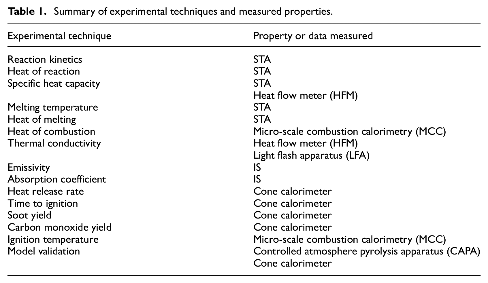
The philosophy that has been adopted in development of this database was driven by the needs of the end users of the properties and fire test data. The most complicated representations of the solid phase in high fidelity fire models, for example FDS, FireFOAM, and ANSYS Fluent, are comprehensive pyrolysis models that represent the major phenomena which drive ignition and involvement of materials in flame spread and fire growth. The comprehensive pyrolysis models require the most material properties and fire test data, but the data collected in the set of experiments required for these models may also be analyzed to yield the input parameters for lower fidelity models, for example CFAST and algebraic correlations. This fact has led to the development of a set of experimental procedures in which thermal analysis data, temperature-dependent thermo-physical properties, spectrally resolved optical properties, and bench-scale burning characteristics were measured. Providing images, a thorough description of each tested material, and all raw measured data and analysis routines were prioritized to maintain transparency of and access to the data. Table 1 provides a summary of the experimental techniques and the data and properties determined through each method.
Summary of experimental techniques and measured properties.
The material characterization methodology took on a hierarchical approach that advanced according to the scale of the sample. 29 This methodology began with experiments on samples prepared at the milligram scale to eliminate the effect of heat and mass transport on the measured quantities and to isolate the kinetics and energetics of thermal decomposition. After milligram-scale experiments, the approach advanced to experiments on gram-scale samples to quantify the effects of heat transport to and through the material. In the final stage of the presented methodology, bench-scale burning experiments were conducted to provide data that may be used to validate the entire parameter set at a realistic scale and may also be directly input into models.
The database includes material property and fire test data from the most common materials encountered in the built environment as informed by a technical panel of fire researchers, fire investigators, and fire safety engineers. 30 In its current state, the data in the database are primarily derived from thermal analysis and bench-scale experiments on individual materials. As this effort continues, there are plans to populate the database with bench-scale data on more individual materials, composite assemblies composed of characterized materials, samples representative of common consumer products, and data collected under expanded conditions (various oxygen concentrations and other experimental conditions). In addition, there are plans to incorporate data from intermediate-scale flame spread experiments as well as large-scale calorimetry data on various upholstered furniture items and other consumer goods. The intent of this database is to provide reliable input data for all fire modeling needs in an interactive format that will be available to investigators, researchers, and other model practitioners in perpetuity.
Experimental Methods
The following sections detail the experimental apparatus and procedures used to obtain material property and fire test data. The sections are presented in the general order in which the experiments were conducted according to the hierarchical methodology mentioned in the ‘Material Database History’ section.
Density
The density of all materials was determined by directly measuring the mass and volume of at least three samples. When possible, samples were prepared into prismatic geometries to make the volume measurement straightforward. After preparing prismatic samples, the samples were conditioned according to the specific protocol for each experimental method, and the volume and mass of the samples were measured.
Moisture content
The temperature and humidity at which materials are stored and have reached equilibrium prior to being tested to measure a specific property have a marked effect on the thermo-physical properties and the fire response of the material. This effect is most notable for lignocellulosic materials, but has also been observed with porous building materials, textiles, and some polymers. When possible, the moisture content of the sample material was measured prior to standard testing. For tests conducted with the heat flow meter (HFM), which is a non-destructive test, the density of the samples was measured, the tests were conducted, and then samples were stored in an oven at a temperature of 105°C for a minimum of 48 h until the mass of the sample stabilized. The resulting samples were considered to have reached equilibrium with the dry environment in the oven, and the density of the samples was measured. The difference in mass of the samples in the dried and non-dried state was attributed to absorbed water and was directly used to calculate the moisture content of the non-dried samples.
Material samples were conditioned for cone calorimeter tests in a conditioning chamber held at 50% relative humidity (RH) and 20°C for a minimum of 24 h and long enough for the mass of the samples to stabilize. The moisture content of the cone calorimeter samples was determined relative to the measured density of the dried heat flow meter samples.
The mass of each sample material was measured with respect to temperature in simultaneous thermal analysis (STA) experiments, and the sample mass for all the tested materials was expected to be stable up to the boiling point of water, so the mass of the sample lost from the beginning of the experiment to approximately 100°C was attributed to moisture loss and was directly used to determine the moisture content of the material.
STA
Thermal analysis experiments rely on the assumption that the sample is sufficiently small that thermal and mass gradients are negligible throughout the experiment, which is equivalent to the assumption that transport processes are also negligible. Thermal analysis experiments typically consist of a sample with a mass on the order of a few milligrams heated along a well-defined temperature program in a well-defined gas atmosphere. Thermogravimetric analysis (TGA) is a thermal analysis technique which involves the measurement of mass, and differential scanning calorimetry (DSC) involves the measurement of heat flow to the sample material. Both methods quantify the evolution of the measurand with respect to temperature.
A NETZSCH STA 449 Jupiter F3 Simultaneous Thermal Analyzer (STA) was used to simultaneously conduct TGA to determine the kinetics of thermal degradation and DSC to determine specific heat capacities, heat of reaction, melting temperature, heat of melting, and the heat of gasification for materials. The STA incorporated a heat flux style DSC measurement. The apparatus consists of a twin-style sample carrier with a space for a reference crucible and a sample crucible. The crucibles are placed in the same position and orientation on the carrier to ensure consistent heat flow rate measurements. A thermocouple welded to the bottom of each carrier position measures the temperature of each crucible. The carrier system is encompassed in a furnace and the apparatus incorporates mass flow controllers to maintain well-characterized gaseous composition and flow conditions while the furnace maintains a well-characterized temperature.
A recent study concluded that the sample preparation method for STA experiments may have a significant effect on the data collected and parameters derived from the data. 31 The major conclusions from the study indicated that samples must be homogeneous, representative of the material to be modeled, and achieve effective and consistent thermal contact with the surface of the crucible adjacent to the thermocouple. To this end, the material samples were prepared into powders using a cryogenic mixing ball mill which ground the samples for a minimum of 10 min. An effort was made to avoid over-grinding to prevent mechanical damage from affecting the molecular structure of the material. Powdered samples were stored in a desiccator in the presence of Drierite for a minimum of 48 h prior to STA experiments to minimize the impact of moisture on the experimental data.
The calibration procedures for the STA are detailed in the MaP Database Technical Reference Guide. 32 Tests were conducted at heating rates of 3°C min−1, 10°C min−1, and 30°C min−1 based on recommendations from the International Congress on Thermal Analysis and Calorimetry (ICTAC). 33 The crucible lid was placed on the sample crucible, and the edge of the sample crucible was marked to ensure consistent orientation of the crucible relative to the sample carrier. All the data currently in the database were collected in experiments conducted in a nitrogen atmosphere with a total flow rate of 70 mL min−1. The temperature program for the STA experiments consisted of an isotherm for 10 min at 50°C followed by a linear increase in temperature at the constant set-point heating rate to the maximum temperature set point (chosen to ensure decomposition was complete) followed by a 5-min isotherm at the final temperature. The experiment was conducted without a sample in the crucible to collect correction data which accounted for buoyancy in the mass measurement and any imbalance between heat flow to the sample and reference crucibles. The entire experiment was repeated with a sample in the crucible to collect data on the sample material. The sample preparation procedure for STA tests involved spreading a powdered sample of the material with a mass of (4.0 ± 0.1) mg evenly across the bottom of a platinum-rhodium crucible. The analysis involved subtracting the correction data from the sample data.
The data presented in the database were collected from STA tests conducted with two different types of furnaces. At the beginning of the project, all experiments were conducted using a silicon carbide (SiC) furnace, and later in the project, a platinum (Pt) furnace was used. The systematic uncertainty in the mass measured in STA experiments is ±2% for the experimental data presented in the database. The total systematic uncertainty in heat flow rate measurements made with the STA was 2.8% for experiments conducted with the Pt furnace and 6.1% for experiments in the SiC furnace. A detailed discussion of the uncertainty in STA measurements is provided elsewhere. 32
Micro-scale combustion calorimetry
A Fire Testing Technology microscale-combustion calorimeter (MCC) was used to measure the HRR of the pyrolyzate evolved during gasification of the sample material with respect to the sample temperature. The apparatus consists of a flat sample platform sized for a single crucible. Experiments were performed in general accordance with Method A described in ASTM D7309. 34 During a test, the crucible is heated in a pyrolyzer furnace that is constantly purged with nitrogen. The pyrolyzer furnace temperature is increased through a linear heating program. The evolved pyrolyzate flows to a combustion chamber which is held at 900°C and where excess oxygen is injected to ensure the pyrolyzate undergoes complete combustion. The gas effluent flows to an oxygen sensor where the decrease in oxygen concentration is measured and related to the HRR through the principle of oxygen consumption calorimetry. Sample specimens were prepared identically to those for the STA experiments to ensure the data collected in each experiment could be directly compared. Powdered samples were stored in a desiccator in the presence of Drierite for a minimum of 48 h prior to MCC experiments to minimize the impact of moisture on the experiments.
The calibration and validation procedures that were followed for the MCC prior to collecting data for the database are detailed elsewhere.32,35 A powdered sample of the material to be tested with a mass of (4.0 ± 0.1) mg was spread evenly across the bottom of the ceramic crucible. The sample and crucible mass were measured prior to testing. Tests were conducted with a heating rate of 30°C min−1 with an initial temperature of 50°C and a maximum temperature that was typically 750°C. Tests were conducted with samples in ceramic crucibles with no lids to ensure there was no added resistance to flow of pyrolyzate gases and vapors from the sample to the combustion chamber. All the data currently in the database were collected in experiments conducted in a nitrogen atmosphere with a total flow rate of 80 mL min−1. The temperature of the combustion chamber was set to 900°C, and the oxygen flow rate to the combustion chamber was 20 mL min−1. After the sample reached the maximum temperature, the sample and crucible were allowed to cool and the mass of the crucible and residue was measured to determine the char yield.
The expanded systematic uncertainty in the HRR measured with the MCC is approximately ±6.5%. The details of the derivation of this uncertainty and a discussion of the components of uncertainty are provided in a related report. 32 The expanded systematic uncertainty calculated for the MCC may be compared with an expanded repeatability (k = 2) of ±2.4% and an expanded reproducibility of ±12% in the HRR determined through an interlaboratory study.34,36
Heat flow meter
A TA Instruments FOX 200 HFM was used to measure the thermal conductivity and specific heat capacity of the materials in the database. Thermal conductivity was measured according to ASTM C518, 37 and specific heat capacity was measured according to a modified version of ASTM C1784. 38 The apparatus consists of two plates between which a 0.20 m × 0.20 m sample specimen is placed. During a test, an actuator above the upper plate moves the upper plate until contact is made between the upper plate and the sample specimen. The instrument measures the distance between the two plates as the thickness of the material. The temperature of each plate is controlled with Peltier coolers and resistance heaters. The heat flow through each plate is measured with thermopiles and the measured quantity may be related to the thermal conductivity or the specific heat capacity of the material, depending on the relationship between the set temperatures of each plate.
Samples were cut square with a side of 0.20 m and tested in the unconditioned as-received state. After testing in the as-received state, the sample specimens were dried in a convection oven at a temperature of 105°C for a minimum of 48 h until the mass of the dried samples no longer changed. If the mass of the dried samples did not change from the as-received state, it was assumed the material did not absorb moisture. The mass of each sample and the calculated density was recorded prior to each HFM test. Sample materials that could not be made into specimens with the desired outside dimensions were cut as large as possible, and the remainder of space in the HFM was filled with the same material.
The HFM was calibrated with several calibration standards procured from or that could be traced back to the NIST. NIST 1453 expanded polystyrene standard reference material (SRM) and a NIST 1450e fibrous glass board SRM were used to calibrate the instrument for thermal conductivity determination. A NIST 1450b SRM (fibrous glass board) was used to calibrate the instrument for specific heat capacity determination. The calibration procedures are detailed elsewhere. 32
ASTM C518 tests were conducted to measure the thermal conductivity. These tests consisted of setting the temperatures of the cold and hot plates such that there was a difference of 20°C and allowing the system to achieve equilibrium. When using the 1453 SRM, the first set of temperatures was 5°C and 25°C and the second set was 35°C and 55°C for the cold and hot plates, respectively. The instrument alternated between these set points three times to collect necessary statistics on the measured thermal conductivity of the sample specimen at mean temperatures of 15°C and 45°C. When the calibration from the 1450e SRM was used, the first set of temperatures was 5°C and 25°C and the second set was 55°C and 75°C for the cold and hot plates. This yielded thermal conductivity values at 15°C and 65°C.
Modified ASTM C1784 tests were conducted to measure the specific heat capacity. These tests consisted of setting both the cold and hot plates equal to the same temperature and allowing the entire system to reach thermal equilibrium. When equilibrium was achieved, both plates were adjusted to the next highest set-point temperature. The total energy required for the system to achieve equilibrium at the next set-point temperature was measured and used to calculate the volumetric heat capacity of the specimen assigned to the mean temperature between the two set-point temperatures. The set-point temperatures defined for data collected for the database were 5°C, 15°C, 25°C, 35°C, and 45°C, which yielded heat capacity values at 10°C, 20°C, 30°C, and 40°C.
A discussion of potential sources of error and uncertainty is provided in ASTM C518 37 and in the FSRI MaP Database technical reference guide. 32 Based on these discussions, the estimated expanded systematic uncertainty in HFM measurements is ±4%.
Light flash apparatus
A Netzsch light flash apparatus (LFA) 467 HT Hyperflash LFA was used to measure the thermal diffusivity of material samples at elevated temperatures. Thermal diffusivity was measured in general accordance with ASTM E1461-13.
39
These tests involved first heating a disk-shaped sample to a series of pre-determined temperature values. Once stable, the front face of the sample was subjected to a high-intensity short duration pulse of radiant energy from a Xenon light source. The temperature of the rear face of the sample was measured using a liquid nitrogen-cooled indium antimonide (InSb) infrared detector. The thermal diffusivity of the material was calculated based on the rate of temperature increase. In the simplest correlation, thermal diffusivity,
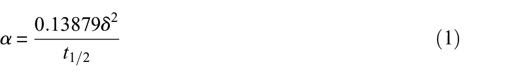
Cylindrical disks of the sample material were prepared with diameters of either 12.7 or 6.0 mm and thicknesses typically in the range of 0.5–3.0 mm were coated with approximately 5 µm of graphite to ensure that all the source infrared radiation was absorbed at the surface and that the infrared detector accurately measured the temperature at the back surface. The temperature set points used for material samples typically ranged from 50°C to the onset of decomposition. Thermally and structurally stable char samples have also been tested although the temperature range has not been standardized for the FSRI MaP Database. Experiments were conducted in triplicate on each sample at each set-point temperature.
A discussion of potential sources of error and uncertainty is provided in ASTM E1461-13. 39 Based on this discussion and guidance from the manufacturer, the estimated expanded systematic uncertainty in thermal diffusivity measurements is ±5%.
Fourier transform infrared spectrometer
A Bruker A562-G gold-coated integrating sphere (IS) accessory on a Bruker Invenio-R Fourier Transform Infrared Spectrometer (FTIR) was used in conjunction with a liquid nitrogen-cooled Mercury Cadmium Telluride (MCT) detector to measure diffuse reflection and transmission for the materials in the database. The FTIR spectrometer uses optical components and the principle of interferometry to quantify the interaction of electromagnetic radiation with materials in the infrared range with respect to the wavelength of the electromagnetic radiation. Spectral reflectance was measured in general accordance with ASTM E903. 40 Specimens for the IS experiments were cut into 0.025 m diameter cylindrical samples, and the exposed surface of the sample was unchanged from the as-received state to ensure the optical properties were representative of the materials encountered in practice.
The daily calibration and validation process is detailed elsewhere. 32 The IS experiments consisted of a series of consecutive tests in which the spectral reflectance was measured for a reference standard, followed by a spectral reflectance measurement for the sample material. The reference standard used in these experiments was a light trap that represented the lowest possible reflectance that could be practically measured at all wavelengths. Tests were conducted with the MCT detector scanning at a rate of 40 kHz for a total of 256 scans per test. Eight replicates of the series which consisted of a reference test followed by a sample test were conducted for each material to collect statistics on the optical properties of the material.
When it was apparent that the sample material was non-opaque to the incident electromagnetic radiation in the infrared range, the transmittance through the material was also measured in IS experiments. For the transmittance experiments, samples of several thicknesses of the material up to approximately 0.006 m were prepared for testing. Each sample was mounted on a sample holder that held the sample at the entrance port to the IS such that the beam passed through the sample prior to entering the IS. Prior to the sample test, a reference test was conducted with no sample in the holder. Diffuse gold surface reference objects were placed at all other ports during these experiments. These data were used to calculate the absorption coefficient of the material.
A comprehensive discussion of sources of uncertainty for IS reflectance measurements with the Bruker A562-G IS is provided by Blake et al. 41 as well as in works related to the database.32,42 To summarize these discussions, sources of systematic uncertainty include deviations from ideal geometry of the sphere and the sample that are not accounted for in theory and analysis. The total uncertainty due to these systematic components is approximately ±4%.
Cone calorimeter
Bench-scale ignition and burning experiments were conducted with a Deatak CC-2 Cone Calorimeter. The cone calorimeter is a standard test apparatus
43
that utilizes oxygen consumption calorimetry to provide data on the HRRPUA of a sample material subjected to a well-defined external heat flux and under flaming conditions. The cone calorimeter features a truncated conical heater with the bottom surface parallel to and 0.025 m above the surface of a 0.1 m square sample. The standard test features a spark igniter that ignites gaseous pyrolyzate when the concentration of gases 0.013 m from the surface of the sample exceeds the lower flammability limit. The mass of the sample is measured through the duration of the test and the gaseous effluent is pulled into a ventilation system at a well-defined flow rate. A gas sampling system measures the reduction in oxygen and increase in carbon dioxide and CO from baseline conditions over the duration of the test. A laser system measures the optical density of the effluent throughout the duration of the test, which can be directly related to the specific extinction area and smoke yield per mass of sample lost. Experiments were conducted to measure the HRRPUA,
Samples were cut into 0.1 m square specimens and stored in a conditioning chamber at 50% RH and 20°C. The mass and dimensions of the sample specimens were recorded, and pictures were taken of the specimens prior to testing. Pictures were also taken after the tests to provide context for the collected data. When layered or composite materials were tested, each layer was characterized according to the full protocol described in the previous sections to help identify and account for the data collected and phenomena observed in cone calorimeter tests. The edges of the sample specimens were wrapped with aluminum foil such that only the top surface was exposed. The sample specimen was placed on a minimum of 0.025 m thick refractory blanket insulation. Every effort was made to avoid the use of the edge frame and the retaining grid to limit unnecessary thermal mass that is difficult to represent in fire models. When samples deformed rapidly on exposure to the heater or intumesced, low mass tie wires were used to maintain the sample in place. When the tie wires were unable to keep the sample specimen in place, the retaining grid was used. When the retaining grid was required, the time to sustained ignition was verified against at least one test conducted without the retaining grid.
The cone calorimeter was calibrated according to the standard calibration procedures 43 prior to testing each day. Cone calorimeter tests were conducted in triplicate with incident heat fluxes of 25, 50, and 75 kW m−2. The sample specimen was observed throughout the test and records were made for the times at which off-gassing started, flashing was observed, sustained ignition was observed, and other pertinent phenomena were observed. The test was allowed to continue until the average MLR dropped below 2.5 gm−2s−1 for 60 s, or was allowed to progress for a maximum of 20 min if ignition never occurred and a maximum of 60 min if ignition did occur. 43
Possible sources of uncertainty and error are discussed in the MaP Database Technical Reference Guide. 32 The total expanded systematic relative uncertainty of the HRR measurement has been estimated as between 5.5% and 7%.44,45 The ASTM E1354 43 and ISO 5660-1 46 standards each report the results of interlaboratory studies on repeatability and reproducibility for the measurements made with the cone calorimeter. The published repeatability and reproducibility values are typically much larger than the estimated systematic component of the total expanded uncertainties, which indicates there is significant scatter due to variation in materials, apparatus, and user procedures.
Controlled atmosphere pyrolysis apparatus
The controlled atmosphere pyrolysis apparatus (CAPA) is a custom-built apparatus first developed at the University of Maryland which was designed to investigate the pyrolysis of solid materials under anaerobic conditions. 47 The dynamic mass of a sample and the unexposed side surface temperatures are measured when the sample is exposed to set incident radiant heat flux. This enables the determination of thermal transport properties through an inverse analysis process using characterized boundary conditions. Experiments conducted with the CAPA also result in data that may be used to validate the complete set of material properties through comparison of mass and MLR data with computational simulations of the experiment.
The CAPA geometry is axisymmetric to allow for simplified modeling and boundary conditions that were easier to represent than those of other bench-scale experiments. CAPA features a truncated conical heater, the same as that used in the cone calorimeter, placed horizontally and parallel with the exposed sample surface and 40 mm above the surface of the sample. The heater is mounted on a linear slide to allow it to be moved over the sample nearly instantaneously and is capable of producing heat fluxes of up to 80 kW m−2. The volume of gas around the sample is purged with 185 L min−1 at 293 K (SLPM) of dry nitrogen to ensure anaerobic conditions and to prevent flaming combustion. Water-cooled chamber walls provide constant temperature boundary conditions, and a black coating on the walls reduces the effect of reflected radiation on the sample. An extensive set of characterization work has been performed to understand the thermal environment to which the sample is exposed during a test.47,48 A balance records the mass of the sample as it decomposes, and an infrared camera records the temperature of the unexposed (bottom) side of the sample.
Samples were cut into 70 mm disks and stored in a desiccator at <10% RH and 23°C for a minimum of 48 h. Samples were adhered to 0.0254-mm-thick copper foil using a well-characterized epoxy to provide an oxidative barrier and consistent substrate. The bottom surface of the copper foil was coated with a high-temperature high-emissivity paint 42 for the purposes of obtaining accurate temperatures through infrared thermography. The edges of the copper foil were wrapped around a copper ring and placed within rings of Kaowool PM insulation sized so that the surface of the sample was flush with the top of the sample cup.
The mass and dimensions of the sample were measured, and photographs were taken prior to the experiment. Gas flow to the chamber was started and allowed to run for several seconds, and the balance was zeroed. The sample assembly was then placed in the chamber, and data acquisition was started. Background data were collected for 1 min before the heater was moved into place over the sample. The test was allowed to continue until mass loss ended. The heater assembly was moved away from the sample to terminate the test. Critical observations during the test were noted. Final background data were collected until the temperature of the back surface of the sample dropped below 100°C. After the test, the residual mass was recorded independent of the CAPA balance, and the post-test sample was photographed.
A comprehensive uncertainty analysis of CAPA has not been performed; however, the uncertainty of various components may be quantified. The expanded uncertainty of the heat flux set point is within
Data analysis
In each of the following sections, example data collected on a general transparent polycarbonate are provided to illustrate the analytical methods and final results of analysis for sample materials. Poly(bisphenol A carbonate), commonly known as polycarbonate, has a repeating unit with a chemical formula of
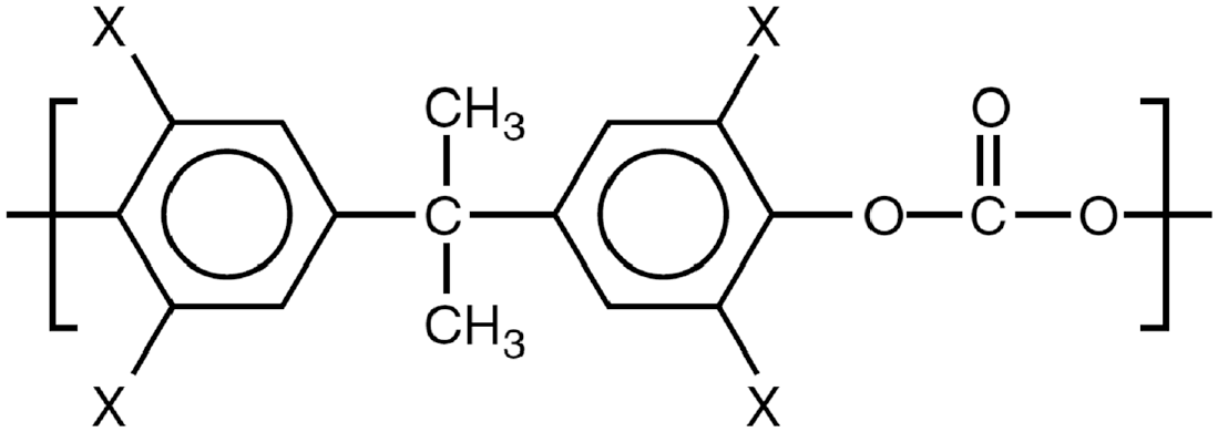
Repeating unit of polycarbonate. 49
The polycarbonate was procured as a 5.4-mm-thick extruded sheet manufactured by PALRAM with the trade name PALSUN Basic. Sample sheets of additional thicknesses were also procured for transmittance testing. According to the supplied safety data sheet, the formulation includes greater than 1% bisphenol-A by weight. The material was transparent to visible light, and the density provided by the manufacturer was 1220 kg m−3. Polycarbonate is a general polymer which is commonly found in many applications in the built environment.
Uncertainty
The data presented in tables and charts in the following sections are associated with mean values of repeated experiments and tests. Unless otherwise noted, the uncertainties presented in the following sections have been calculated as the standard deviation of repeated measurements with a coverage factor of 2 such that they encompass 95% of the expected data. For single-value quantities presented in tables, the uncertainties have been rounded according to the appropriate significant figures. The solid lines in charts are associated with the mean value of repeated measurements, and the error bars and shaded regions are representative of the aleatoric or random component of the total uncertainty; the total expanded uncertainty requires this component to be added in quadrature with the systematic uncertainty. Systematic uncertainties associated with each apparatus have been discussed in the previous sections.
Density
Mass and volume were directly measured, and no additional analysis was required to calculate a final value for density. The density of the polycarbonate samples was measured as (1220 ± 12) kg m−3. Upon heating three individual samples at 105°C for 2 days, the masses of the samples did not change, and it was concluded the material did not absorb moisture and that the samples that were tested had a moisture content of approximately 0%.
Reaction kinetics
The most common method in fire modeling to describe the temperature dependence of the MLR of a material is by adopting the definition of the reaction rate from chemistry. Chemical reaction rates are typically described using the Arrhenius equation. Equation (2) presents the general form of the reaction rate equation that is (or a modified form of which is) commonly invoked in pyrolysis models to describe the evolution of the composition of the material and its production of gaseous volatiles. The equation describes the jth reaction that involves the ith reactant. The Arrhenius reaction parameters, which include the Arrhenius pre-exponential factor
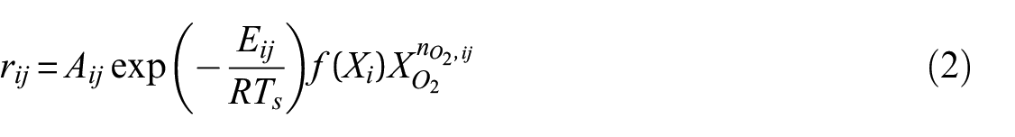
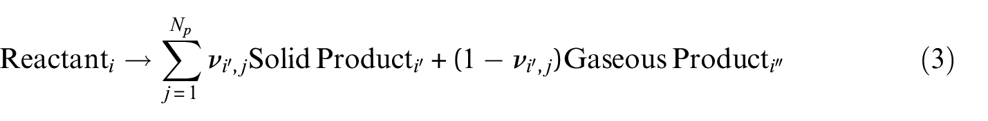
At present, oxidative pyrolysis and oxidation have not been extensively studied or quantified for the database, and all thermal analysis data were collected in a nitrogen atmosphere, which takes the volumetric oxygen concentration to zero in equation (2). It was also assumed that all reactions were of the first order. This eliminated the need to determine the reaction order without significantly affecting the curves generated with the kinetic parameters. The default reaction scheme for all materials involved sequential reactions where a single solid reactant was typically converted to a single solid product and a single gaseous product as shown in equation (3) where
Part of the argument for defining pyrolysis kinetics in fire modeling is that definition of kinetics effectively decouples the mathematical description of burning from the experimental method, ignition source, or fuel configuration. Kinetics allow the model to be truly predictive by representing the burning rate as a function of temperature only. A factor that complicates the definition of reaction kinetics is that there is no single, universally accepted, standard method in the fire modeling community to determine reaction kinetics, which can lead to a disparity between kinetic parameters determined by different investigators using disparate experimental and analytical methods. The International Association for Fire Safety Scientists (IAFSS) Working Group on measurement and Computation of Fire Phenomena (MaCFP) Condensed Phase Phenomena Subgroup has illustrated the variety of results obtained when disparate experimental and analytical methods are adopted. 50
There are many model-free methods (i.e. the form of the function
Model-based methods typically require the practitioner to define a form of the kinetic model to describe the global reaction mechanism. There are no standard model-based methods, and the majority of available methods rely on regression algorithms, optimization algorithms, or otherwise minimization of error between experimental data and model predictions. Different model-based methods have been described by Lautenberger and collegues,54,55 Bruns and Leventon, 23 and Fiola et al. 56
McKinnon et al. described an analysis whereby reaction kinetics parameters determined through several model-free and model-based methods may be displayed on a Constable plot of activation energy versus the logarithm of the Arrhenius pre-exponential factor. 57 In this approach, a model-based nonlinear-least-squares (NLS) algorithm is used to minimize the residuals between normalized mass data collected in a TGA experiment and model-predicted data. TGA data from each experiment conducted at heating rates of 3°C min−1, 10°C min−1, and 30°C min−1 were analyzed individually with the NLS algorithm as well as considering all data sets equally weighted in an objective function. When a single reaction sufficiently described the data, the kinetics were determined using model-free and model-based methods, whereas for materials described by multi-reaction schemes, only model-based methods were used.
Kinetic pairings for polycarbonate are presented in Figure 2, and the kinetic parameters determined through each method for polycarbonate are presented in Table 2. The equation for the regression line which describes the kinetic pairings is
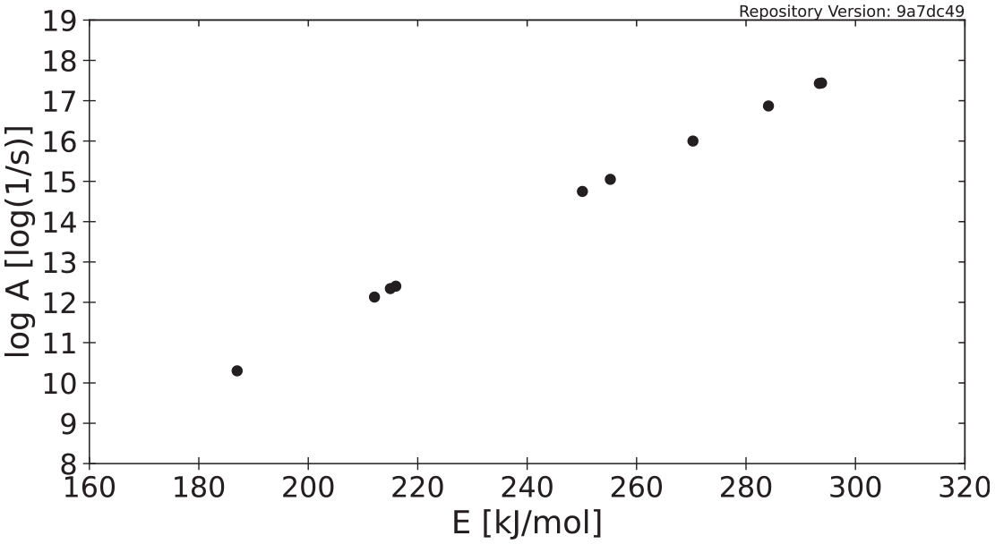
Kinetic parameters determined for polycarbonate.
Kinetic parameters determined for anaerobic decomposition of polycarbonate.
In theory, when defining a single set of kinetics in a model, any value along the line that best fits the kinetic pairs may be used to describe the temperature dependence of mass loss. In practice, this is not necessarily true, as many researchers have shown that even kinetic parameters coupled through the aforementioned relationship can display shifts in temperature and MLR magnitude.60,61 A single set of reaction kinetics may be determined for a burning scenario through an optimization procedure which accounts for the relationship between the kinetic parameters and calibration data from the pertinent experimental scale as described previously. Because of the strong linear relationship between the activation energy and the pre-exponential factor, when representing the uncertainty in the kinetic parameters, care must be taken to ensure the two parameters remain coupled and the relationship is adequately communicated.
Melting temperature
STA data may be used to determine the temperature at which materials melt or their viscosity decreases to allow dripping. By plotting MLR data on the same axes as heat flow rate data, the temperature ranges at which energetic physical transitions that correspond to no mass loss occur may be identified. Melting manifests in heat flow rate data as an endothermic curve that increases from the baseline, reaches a peak, and decreases back to the baseline. This peak is not accompanied by a change in mass. The temperature at which the heat flow rate curve deviates from the baseline is considered the onset temperature for melting, and the temperature at which the maximum endothermic heat flow is measured is considered the peak melting temperature. Both quantities are typically reported as a result of this analysis and have been provided in the database for the materials that undergo melting. The area between the melting peak curve and the heat flow rate baseline is considered the enthalpy of melting. This analytical procedure is described in ASTM E793, 62 ASTM E794, 63 and ISO 11357-3. 64
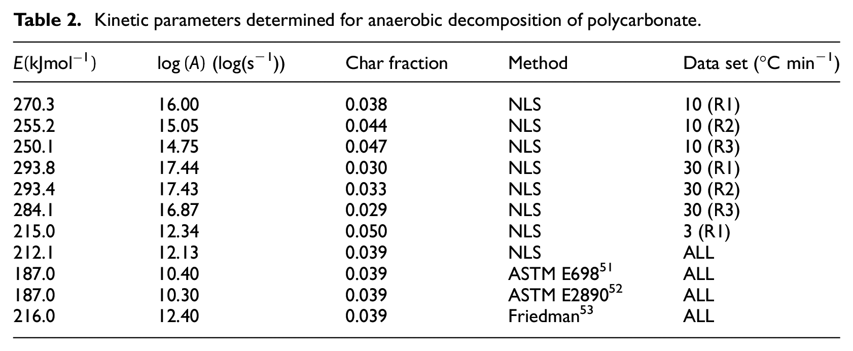
The procedure for determining the peak melting temperature, the temperature at onset of melting, and the limits of integration to determine the enthalpy of melting for the values presented in the database is a multi-step process that begins with identification of the temperature at the melting peak. The temperature at the peak was determined by finding the roots of the derivative of the heat flow rate curve with respect to temperature. After identifying the peak melting temperature, a 150°C window centered at the peak melting temperature was extracted from the heat flow rate data and an iterative polynomial fit algorithm was used with a fifth-degree polynomial to automatically draw the baseline for the extracted data. The process involved iteratively performing polynomial regression and truncating all values in the data above the regression line, which eventually eliminated the peaks and left only the baseline. An example baseline drawn for polycarbonate is provided in Figure 3. The figure also shows the normalized MLR curve collected at 10 to illustrate that the energetic peak was not associated with a change in mass.
Determination of melting temperature and enthalpy of melting for polycarbonate: (a) heat flow rate data for polycarbonate with calculated baseline and melting peak highlighted and (b) normalized MLR collected at 10°C min−1 for polycarbonate.
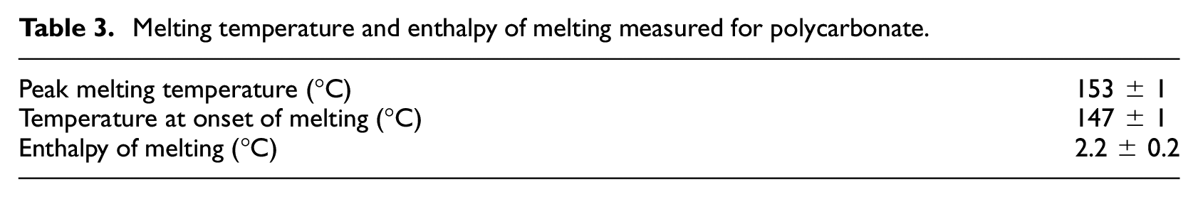
The point at which the data curve deviated from the baseline was determined as the highest temperature below the peak melting temperature at which the two curves intersected and were defined as the temperature at the onset of melting. The point at which the data curve converged back to the baseline was determined in the same way for the temperature above the peak melting temperature at which the curves intersected. The temperature at onset was defined as the lower limit of integration, and the temperature at which the data curve returned to the baseline was defined as the upper limit for the integration. The values measured and calculated for polycarbonate are presented in Table 3.
Melting temperature and enthalpy of melting measured for polycarbonate.
Specific heat capacity
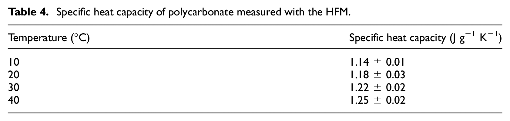
The specific heat capacity was directly measured using the HFM. The maximum sample temperature that may be achieved when measuring specific heat capacity with the HFM is 40°C. Table 4 presents the specific heat capacity measured with the HFM for polycarbonate through the available temperature range. The heat capacity increased with increasing temperature which is consistent with intuition.
Specific heat capacity of polycarbonate measured with the HFM.
Data from STA experiments may also be manipulated to calculate an apparent temperature-dependent specific heat capacity that is valid over a wider range of temperatures. The procedure for calculating the apparent specific heat capacity is a modification of the ASTM E1269
65
standard, and it stems from the energy balance on a sample in a thermal analysis experiment. Equation (4) is the representation of this energy balance. In the equation,
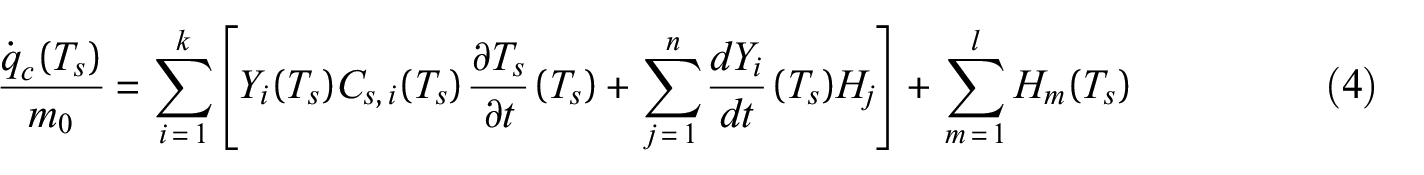
Apparent specific heat may be calculated from data collected over temperature ranges when reactions and melting do not occur. This simplification removes the second and third terms from the analysis and leaves the sensible enthalpy term on the right-hand side. Figure 4 displays the apparent specific heat capacity calculated from DSC data collected with a heating rate of 10°C min−1 over the full temperature range of the experiment and the normalized MLR over the full temperature range to aid in identification of temperature ranges where no mass loss or physical changes occurred. Dividing the measured normalized heat flow rate on the left-hand side by the heating rate
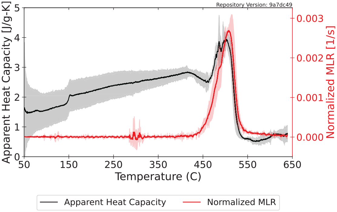
Apparent specific heat capacity plotted with normalized MLR for polycarbonate.
Figure 5 displays the specific heat capacity measured with the HFM and the apparent specific heat capacity calculated from DSC data over temperature ranges where no mass loss occurred. By plotting the data from the DSC and the HFM on the same plot, regression can be conducted to determine a curve that best describes the specific heat capacity of the virgin material from room temperature to the onset of decomposition. Typically, the line of best fit takes a linear form or that of a second-order quadratic, although other power law relationships have also been adopted in common pyrolysis models.
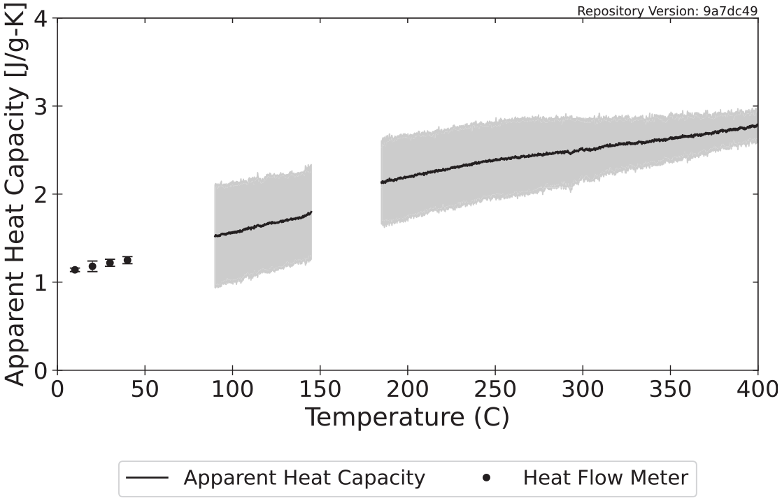
Temperature-dependent specific heat capacity calculated for polycarbonate.
Thermal conductivity
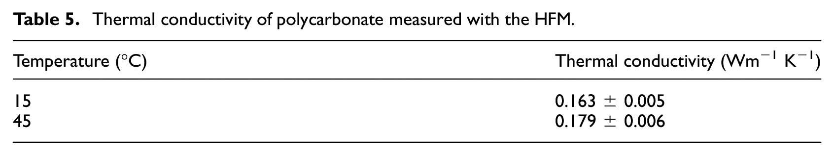
Thermal conductivity was directly measured with the HFM, and no analysis was required to calculate final values from these data. The thermal conductivity values measured with the HFM for polycarbonate are displayed in Table 5.
Thermal conductivity of polycarbonate measured with the HFM.
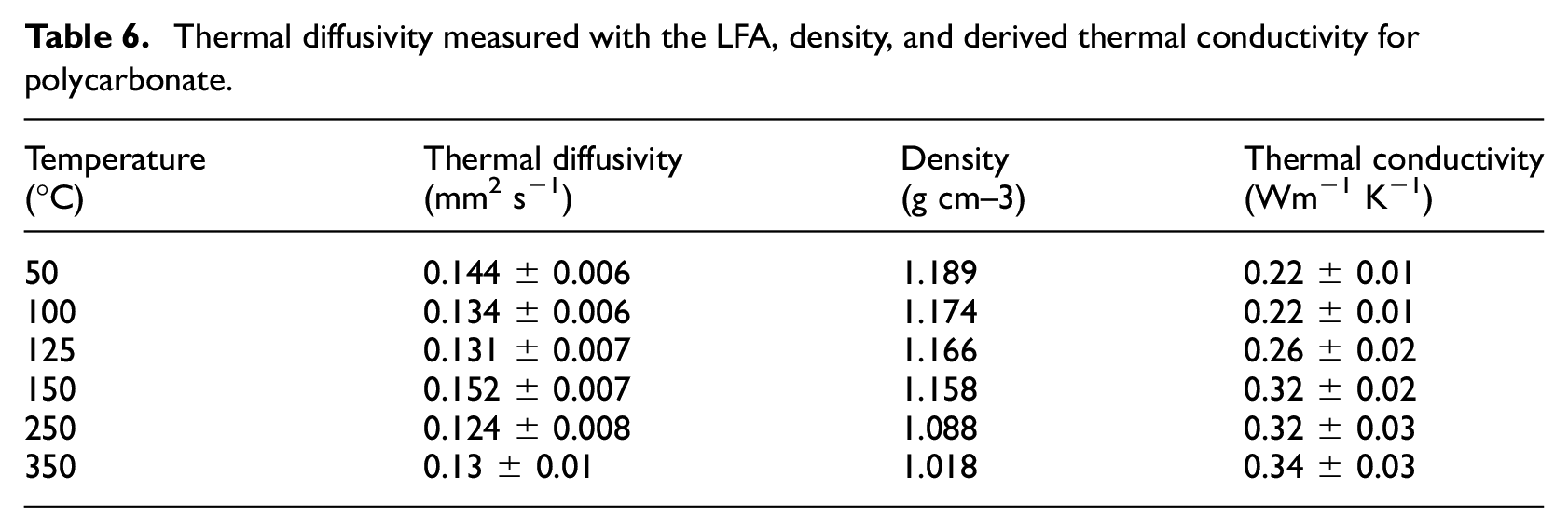
Thermal conductivity was also calculated from data collected in LFA experiments at higher temperatures than were possible in HFM experiments. The thermal conductivity was calculated as the product of the thermal diffusivity, specific heat capacity, and density of the polycarbonate. The thermal diffusivity was measured directly in LFA experiments conducted on samples ranging in thickness from 0.48–2.59 mm. Experiments were conducted with two different sample holders, one was intended for stable samples that did not experience significant dimensional changes through the tested temperature range and the second was intended for liquids and materials that melted in the investigated temperature range. Because the tested polycarbonate was known to melt in the range of 147°C–185°C, samples were tested at temperatures of 50°C, 100°C, and 125°C in the ordinary sample holder and at temperatures of 150°C, 250°C, and 350°C in the sample holder intended for liquids and melts.
The thermal conductivity, k, of polycarbonate was calculated as the product of the thermal diffusivity,

Thermal diffusivity measured with the LFA, density, and derived thermal conductivity for polycarbonate.
Heat of reaction
The heat of reaction (heat of decomposition) is the amount of energy absorbed by a material during a thermal degradation reaction. The heat absorbed by the material during the thermal degradation reaction was determined according to ISO 11357-5
66
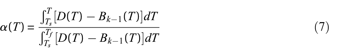
as the integral of the difference between the measured heat flow rate curve and an assumed sensible enthalpy baseline. A form of the baseline which was tangential to the experimental heat flow rate curve at the origin and terminal points of the baseline and defined by equations (6) and (7) was adopted for the analysis. This form of the curve resulted in a monotonically decreasing sensible enthalpy baseline over the course of the thermal degradation reaction. This shape has a physical justification because the mass of the sample and the specific heat capacity of the sample decreased over the course of the reaction. The origin

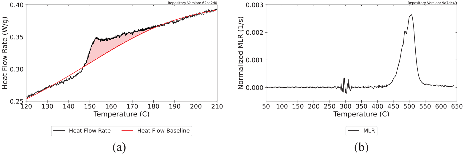
Representative heat flow rate data collected at a heating rate of 10°C min−1 are plotted with the sensible enthalpy baseline in Figure 6. The heat flow rate data are presented on an initial mass basis, which means the integral must be corrected to represent the total mass lost in the reaction. The mass basis for all integrals was converted from the initial mass to the total mass lost over the temperature range that corresponded to the limits of integration. To provide an example, this analysis was performed for the data collected in all STA experiments. The mean heat of reaction calculated for polycarbonate at each heating rate is provided in Table 7.
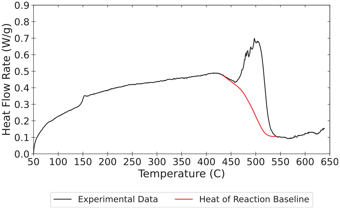
Heat flow rate data and sensible enthalpy baseline calculated for polycarbonate at 10°C min−1.
Heat of reaction calculated for polycarbonate.
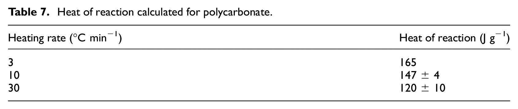
Although there is variation in the heat of reaction for polycarbonate with the heating rate, this is not an expected effect. These variations are likely artifacts of deviations from ideal behavior in the STA experiments and the simplified data analysis process. Polycarbonate is known to melt, form bubbles within the melt at the onset of decomposition, and result in an intumescent residue as a product of thermal decomposition. All of these processes may effect the thermal contact between the sample material and the temperature-sensing surface of the crucible and cause error in the heat flow measurement. These effects are minimized through calibration and careful selection of sample mass and heating rates, but it is impossible to eliminate them. An additional likely source of variation in heats of reaction is the relatively simplistic baseline drawn for analysis which does not account for the actual evolution of the specific heat capacity of the sample material through decomposition. The errors due to these factors tend to be amplified at lower heating rates because of the longer durations of the complicating phenomena in lower heating rate tests which get compounded in the integration operation.
Emissivity
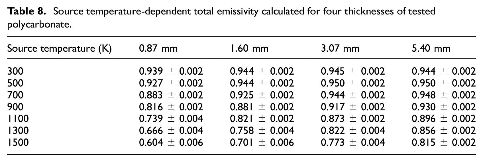
Total emissivity was calculated from spectral reflectance data collected with the IS. The emissivity was taken as equal to the absorptance through Kirchoff’s Law, and the majority of the materials were assumed to act as opaque bodies, which allows definition of the absorptance equal to one minus the reflectance of the material. The materials that were non-opaque to visible light were also assumed to be non-opaque to infrared radiation. For these materials, the absorptance was defined as one minus the transmittance minus the reflectance of the material. For the materials that could not be defined as opaque to infrared radiation, the absorption coefficient was determined according to the analytical procedure presented in the following section. The emissivity was calculated according to equation (8), where
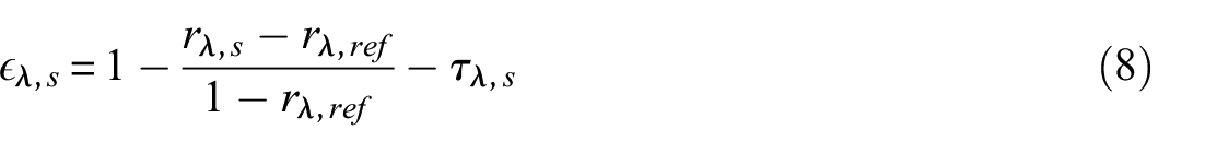
The total emissivity was calculated according to equation (9). The spectral emittance was scaled by an assumed incident spectral distribution in the form of Planck’s law
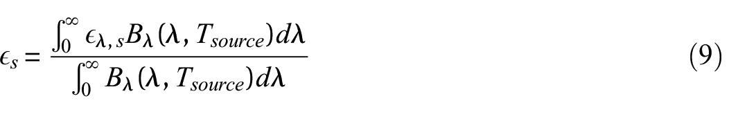
Source temperature-dependent total emissivity calculated for four thicknesses of tested polycarbonate.
Absorption coefficient
For materials that are not opaque to infrared radiation, it is important to quantify the fraction of incident radiation that is transmitted through the material or absorbed in depth. Linteris et al.
68
provided a discussion of attenuation of radiation within a medium. The absorption coefficient is a metric that quantifies the amount of infrared radiation absorbed by a material and may be considered the inverse of the mean penetration depth (m−1) or the same quantity normalized by the density of the material (m2 kg−1). A large absorption coefficient indicates all the radiation is absorbed at the exposed surface of the material or at a small depth into the surface of the material. The form of Bouger’s law that may be applied to describe the transmittance of a material is provided as equation (10), where
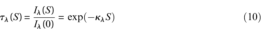
The equation was manipulated into the linear form of equation (11) to simplify determination of the absorption coefficient

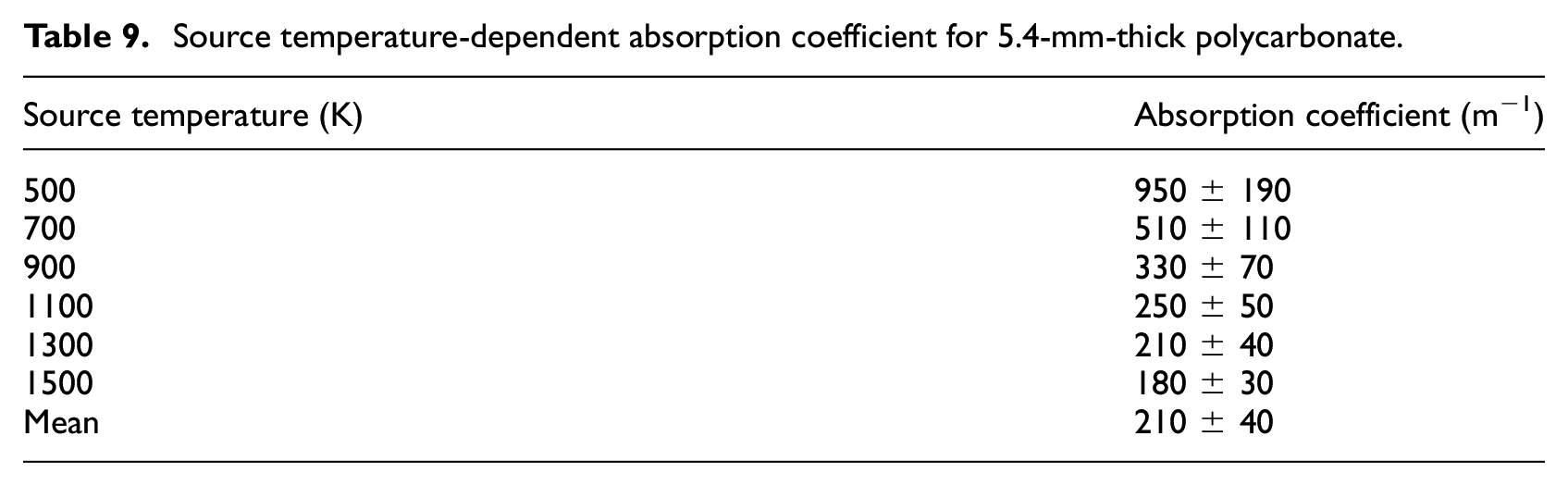
Transmittance was measured for samples of several thicknesses relative to the light trap and complete transmission (no sample in the IS). The total transmissivity was calculated according to equation (9) with the spectral emittance in the equation substituted for the spectral transmittance. The thickness of the sample was plotted against the negative of the natural logarithm of the average total transmittance, and linear regression was performed. The slope of the regression line was taken as the absorption coefficient for the material when exposed to radiation at the specific source temperature. Figure 7 displays an example of the graphical procedure used to calculate the absorption coefficient of polycarbonate for a source temperature of 1500 K and a sample thickness of 3.07 mm. Table 9 displays the source temperature-dependent absorption coefficient calculated for polycarbonate.
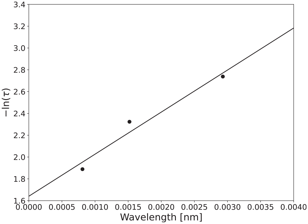
Graphical procedure to determine absorption coefficient for polycarbonate.
Source temperature-dependent absorption coefficient for 5.4-mm-thick polycarbonate.
Heat of gasification
The heat of gasification is defined as the total amount of energy per unit mass required to convert a condensed phase material entirely to the gas or vapor phase. This quantity includes sensible enthalpy (energy required to increase the temperature of the material), heat absorbed during physical transitions, and heat absorbed during decomposition reactions. There are two main approaches to determining the heat of gasification which rely on heat flow rate data collected in thermal analysis experiments and burning rate data collected in bench-scale flammability tests. Only the method that utilizes thermal analysis data is described here and calculated for the FSRI MaP Database. The method which relies on bench-scale flammability test data has been described by several authors.69–71
Stoliarov and Walters 72 described a method for determination of the heat of gasification using heat flow rate data collected in experiments conducted in a power compensation DSC. Although the data provided in this database are from experiments conducted with an STA which incorporates a heat flux DSC, the analytical procedure is the same. The heat of gasification is calculated as the integral of the heat flow rate curve (presented in Wg−1) with respect to time collected in an experiment with a constant heating rate from room temperature to the temperature at which degradation is complete. For the values presented in the database, these integrals were computed over the temperature range of 50°C to the temperature at which the MLR decreased to below 5% of the maximum MLR. For polycarbonate tested at 10°C min−1, the upper-temperature limit was approximately 540°C. The mean heat of gasification calculated for polycarbonate according to the DSC data collected with a heating rate of 10°C min−1 was (1560 ± 150) J g−1. Figure 8 displays the integral of representative heat flow rate data collected on polycarbonate at a heating rate of 10°C min−1.
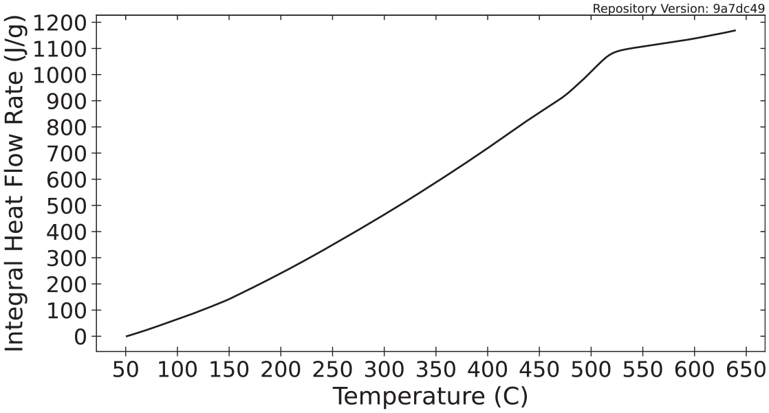
Integral of heat flow rate data used to calculate heat of gasification (initial mass basis).
HRR
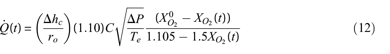
The HRR of the sample materials was measured with oxygen consumption calorimetry using the cone calorimeter and the MCC. The raw oxygen concentrations measured with each apparatus and the analyzed data presented as HRRPUA for the cone calorimeter and specific HRR for the MCC are available in the database. The cone calorimeter measured HRR with respect to time during tests conducted with a set-point heat flux incident to the sample. The MCC measured HRR as a function of temperature.
The equation used to calculate the HRR from cone calorimeter data is presented as equation (12).
The HRR of the sample pyrolyzate produced in the MCC is measured by oxygen consumption flow calorimetry. The equation used to calculate the HRR is provided as equation (13). The density of gaseous products of combustion
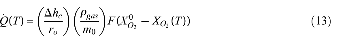
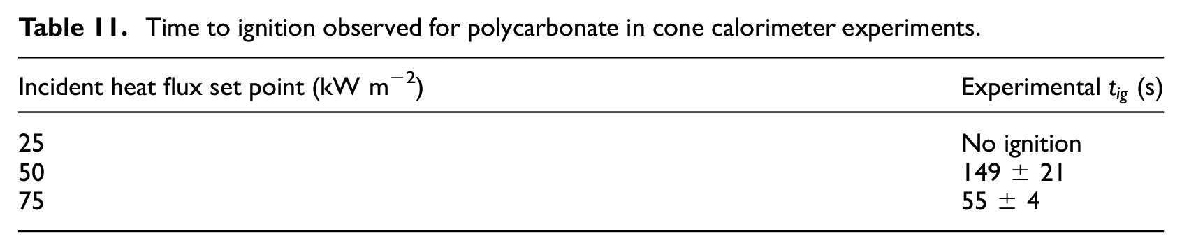
Figure 9 displays the HRRPUA measured for polycarbonate at heat fluxes of 50 and 75 kW m−2 as well as the specific HRR measured in MCC experiments. Polycarbonate samples were tested with the cone calorimeter at a heat flux of 25 kW m−2, but the sample specimens did not ignite and, consequently, did not release any heat during the experiments. The specific HRR has a maximum value of 520°C with a peak magnitude of approximately 234 Wg−1. Although the total heat released in each cone calorimeter experiment is equal, the HRRPUA curves show a trend where the peak HRRPUA increases and the duration of burning decreases with increasing incident heat flux. This phenomenon is explained with an interpretation of the specific HRR curve such that the temperature of the polycarbonate sample exposed to the cone heater increases in temperature more rapidly at higher incident heat fluxes, which more rapidly increases the specific HRR along its curve, ultimately generating higher HRRPUA values and peaks.
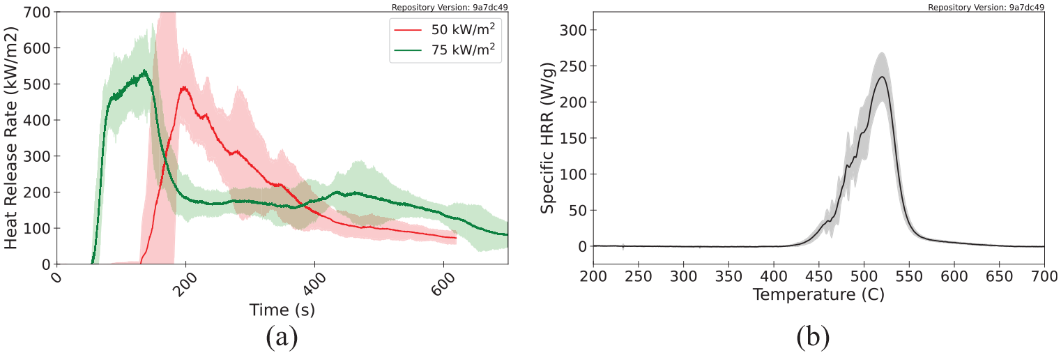
HRR measured for polycarbonate: (a) HRRPUA measured with the cone calorimeter and (b) specific HRR measured with the MCC.
Heat of combustion
The heat of combustion is the amount of energy released when the gases produced during pyrolysis of a material undergo combustion. The heat of combustion is typically presented on a per unit mass of the condensed phase material basis. An effective heat of combustion may be calculated from cone calorimeter data and an effective heat of complete combustion may be determined from analysis of MCC HRR data. Because the cone calorimeter experiments are conducted in an open atmosphere with a potentially turbulent flame and the temperature and oxygen concentration in the MCC combustion chamber are well controlled, the process and efficiency of combustion for these two scenarios are significantly different. Typically, the effective heat of combustion measured in the cone calorimeter incorporates some incomplete combustion that produces soot and CO, and the resultant value is lower than the theoretical heat of combustion. In the MCC, combustion is forced through completion, and so the effective heat of combustion is typically closer to the theoretical value than the effective heat of combustion calculated from cone calorimeter data.
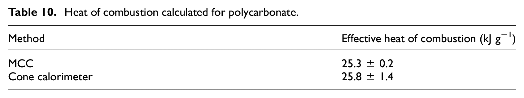
The instantaneous effective heat of combustion may be calculated from cone calorimeter data by dividing the instantaneous HRR by the instantaneous MLR. A representative value may also be determined from the duration of the cone calorimeter test by dividing the total heat released (integral of HRR) by the total mass lost. Because the mass of the sample specimen is not monitored during the test in the MCC, an effective heat of complete combustion may be calculated after a test is completed. The total heat released over the duration of the test is divided by the total mass lost (difference between initial mass and residual mass) to get the heat of complete combustion. Table 10 displays the heats of combustion for polycarbonate calculated with MCC data and cone calorimeter data. Although the heat of combustion determined in the MCC is typically higher than that in the cone calorimeter because the MCC forces complete combustion, the value calculated from cone calorimeter data for polycarbonate is higher than the value calculated from MCC data. This may be caused by char oxidation which occurred in the cone calorimeter tests and was not possible in the MCC tests. The theoretical heat of complete combustion of carbon is approximately 32.8 kJ g−1 which would act to artificially increase the effective heat of combustion for the material.
Heat of combustion calculated for polycarbonate.
Time to ignition
The
Time to ignition observed for polycarbonate in cone calorimeter experiments.
Ignition temperature
The ignition temperature is not an intrinsic property of a material. Materials do not spontaneously ignite at a specific universal ignition temperature. The temperature at which materials ignite is a complicated function of the material properties, geometry, orientation, exposure, and environmental conditions. An ignition criterion that may be more physically justified and appropriate for predictions is one based on a critical HRR or a critical MLR. 13 One method that has been proposed to calculate the ignition temperature relies on data collected in the MCC. Several other methods rely on data collected with the cone calorimeter or similar bench-scale flammability experiments.
A representative ignition temperature is determined from specific HRR data collected with the MCC. Lyon et al. 73 presented a correlation between a critical specific HRR and the temperature for sustained piloted ignition in bench-scale flammability tests. The mean critical specific HRR that corresponds to sustained ignition was found to be (25 ± 8) Wg−1 for 20 different polymers. Assuming this correlation applies to other materials that are not synthetic polymers, it may be applied more generally to identify a range of temperatures at which ignition is likely to occur. A graphical representation of this analysis is displayed in Figure 10. The mean ignition temperature calculated for polycarbonate through this method is 452°C and the range of values defined by the uncertainty in the measured data and the correlation is 442°C to 472°C.
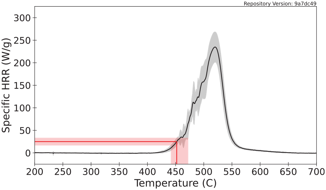
Application of the ignition temperature correlation for MCC data.
There are several other correlations that have been devised to estimate the ignition temperature and time to ignition
Soot yield
The soot yield may be determined from the smoke obscuration measurement in the standard cone calorimeter experiment. Equation (14) relates the intensity of the laser
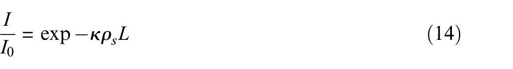
To determine the soot yield, the soot density must be determined from the measured decrease in intensity of the laser due to absorption and scattering. The path length of the laser in the cone calorimeter is 0.11 m, and Mulholland and Croarkin 75 suggest a value of 8700 m2 kg−1 for the average mass extinction coefficient of smoke. The soot density, or mass concentration of soot in air (kg m−3), may be calculated as in equation (15)
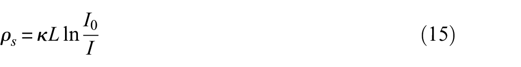
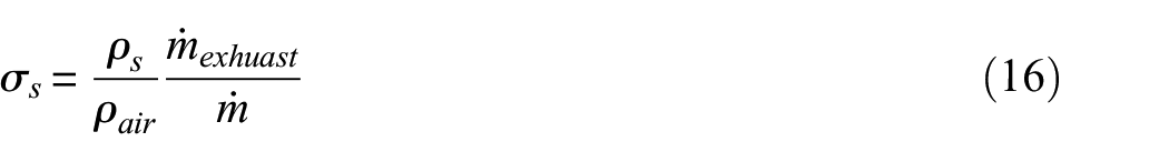
The temperature at the location in the duct where the laser measures the extinction coefficient may be used to calculate the air density. Dividing the mass concentration of soot by the air density yields the mass fraction of soot in the gas mixture. The soot mass fraction may be multiplied by the exhaust duct mass flow rate to yield the total mass flow of soot at a given time in the test. To calculate the soot yield, the total mass flow of soot in the duct is divided by the MLR of the sample such that the units of yield are (kg of soot produced/kg of sample mass lost). Equation (16) presents this calculation where
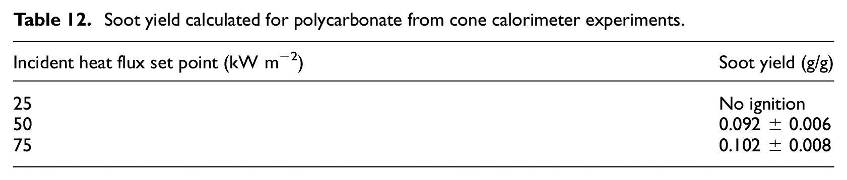
The polycarbonate samples did not ignite when exposed to an incident heat flux of 25 kW m−2 in the cone calorimeter, so Table 12 displays the soot yields calculated for polycarbonate from data collected in cone calorimeter experiments at heat fluxes of 50 and 75 kW m−2. The values that are presented in the table and in the database are calculated by integrating the instantaneous soot mass flow rate from the time at which 10% of the total mass loss has occurred to the time at which 90% of the total mass loss has occurred and dividing by 80% of the total mass lost over the test.
Soot yield calculated for polycarbonate from cone calorimeter experiments.
CO yield
The CO concentration of the effluent collected in the exhaust hood of the cone calorimeter is typically measured during an experiment. This concentration is reported in parts per million (ppm) or as a volumetric concentration. To convert from volumetric fraction to mass fraction, the volumetric fraction must be multiplied by the ratio of the density of CO to the density of air flowing through the duct. This resulting mass fraction is multiplied by the exhaust duct mass flow rate to get the instantaneous mass flow rate of CO. The instantaneous CO yield (kg of CO produced/kg of sample mass lost) may be determined by dividing the mass flow rate of CO in the duct by the MLR of the sample. Equation (17) presents this calculation where
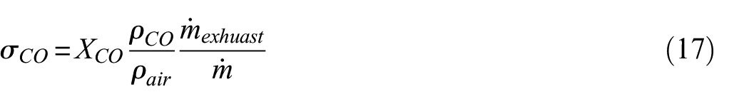
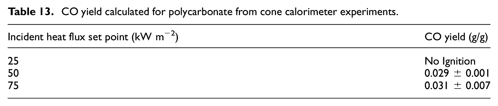
Table 13 displays the CO yields calculated for polycarbonate from data collected in cone calorimeter experiments at heat fluxes of 25, 50, and 75 kW m−2. The values that are presented in the database are calculated by integrating the instantaneous soot mass flow rate from the time at which 10% of the total mass loss has occurred to the time at which 90% of the total mass loss has occurred and dividing by 80% of the total mass lost over the test.
CO yield calculated for polycarbonate from cone calorimeter experiments.
Validation
The development of this database is predicated on the assumption that when a parameter set can accurately describe fundamental quantities in model representations of canonical experiments, the model practitioner may have confidence that the parameter set can describe the same materials and phenomena in larger scales and more complicated burning scenarios. Validation of material property sets typically involves parameterization of a model using the determined properties to define the material and comparison of model results against directly measured experimental data or observations.
Validation of pyrolysis models is an area of active research, and there is not currently a consensus among researchers and model practitioners on best practices for parameter definition or acceptance criteria. Validation for the material properties and reaction parameters presented in the database involve comparison of model predictions of bench-scale experiments against experimental data collected in the same experiments. In the current state of the MaP Database, these bench-scale experiments are conducted with the STA, the cone calorimeter, and the CAPA. The plots presented in this section provide comparisons between experimental data and results of model representations as an example of validation of the properties measured and presented for polycarbonate.
Model parameterization
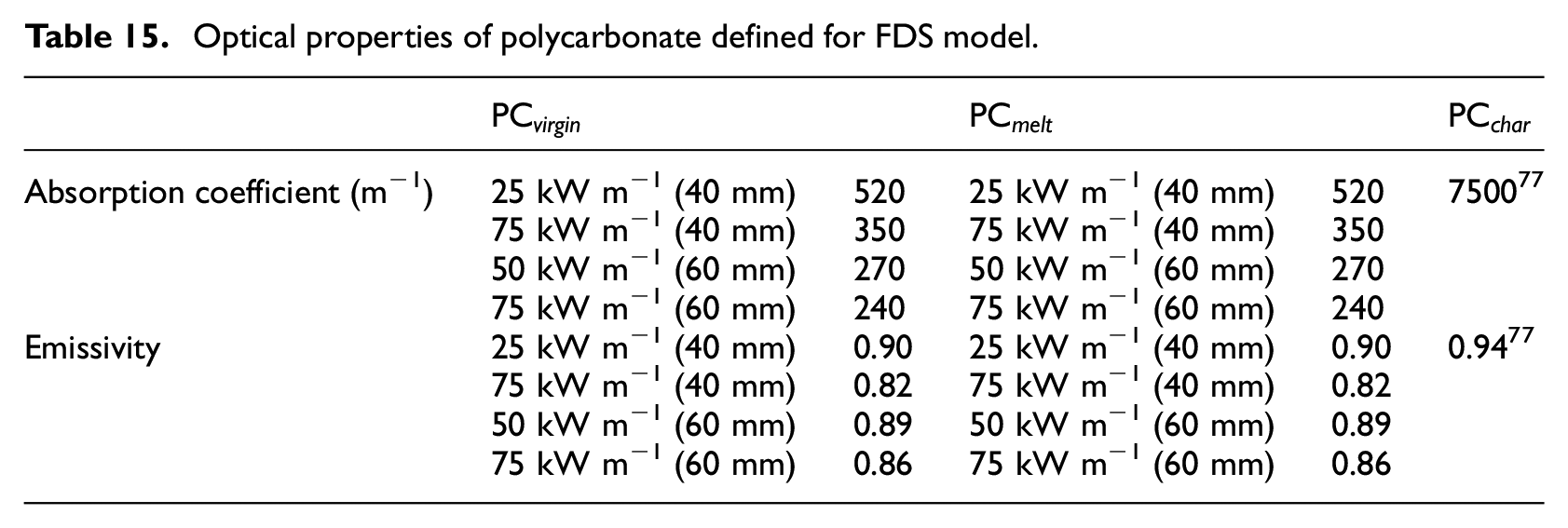
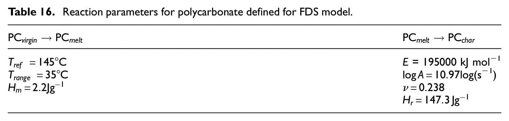
The set of parameters measured in the aforementioned experiments on polycarbonate was used to define the material in a model constructed with FDS (v6.8.0). The model represented only the solid phase with the gas phase represented according to well-defined boundary conditions that were measured or observed during the experiments. A summary of the parameters used to define polycarbonate in the model is provided in Tables 14 to 16. An explanation of the mixture rules and interpolation of thermo-physical properties defined according to temperature-dependent values may be found in the FDS documentation.10,76
Thermo-physical properties of PC defined for FDS model.
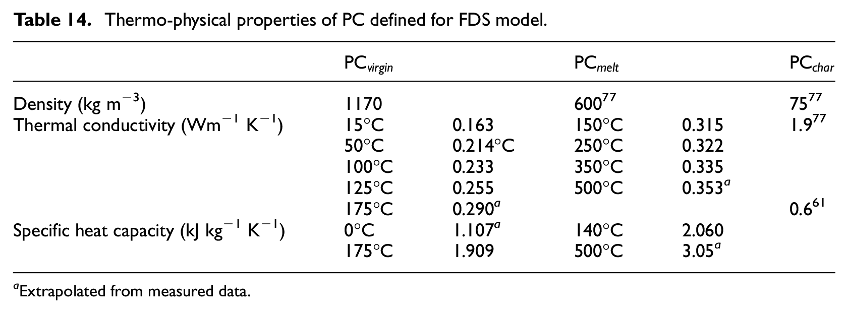
Extrapolated from measured data.
Optical properties of polycarbonate defined for FDS model.
Reaction parameters for polycarbonate defined for FDS model.
The density of the
The spectral reflectance and transmittance data collected on the polycarbonate samples in IS experiments were analyzed to determine effective total emissivity and total absorption coefficient values. Because the polycarbonate samples were partially diathermanous (transmitted some portion of incident infrared radiation), the calculated total emissivity and total absorption coefficient were dependent on the spectral distribution of the incident radiation and the thickness of the material. The source temperature for the spectral distribution used to scale the measured data was estimated according to the set-point heat flux in the cone calorimeter and CAPA tests and the view factor between the cone heater frustum and the sample distances of 40 mm (CAPA) and 60 mm (cone calorimeter), 78 assuming an emissivity of 1 for the cone heater. When data were not collected on samples with a specific thickness, as was the case with the approximately 2.4-mm-thick CAPA samples, the spectral response was interpolated from the two data sets collected at the closest thicknesses.
Although the relationship between the negative logarithm of transmissivity and the optical path length is linear at small sample thicknesses, this relationship is necessarily not highly linear when data from samples above a critical thickness are considered and the fraction of transmitted radiation decreases to either an asymptotic finite amount or to zero. The absorption coefficient is taken as the slope of this linear relationship, so for simulating CAPA samples that were thinner than cone calorimeter samples, only data from samples with thicknesses up to 2.4 mm were considered in the analysis whereas data collected from IS samples up to thicknesses of 5.4 mm were considered for the modeling the cone calorimeter samples. The
Table 16 shows the parameters that define the reactions in FDS. FDS has several methods available for modeling the production of gaseous volatiles and solid-phase reactions, each with its own set of parameter requirements. One method requires definition of the a reference peak temperature, the temperature range corresponding to the reaction, and, optionally, the reference peak MLR. This method was adopted to describe the transition from
STA—MLR
The reaction kinetics determined for polycarbonate assuming the simplistic reaction model described in an earlier section may be validated against experimental MLR data collected in STA experiments. Figure 11 shows the predicted nMLR in a simulated STA experiment compared against the experimental data collected at heating rate set points of 3°C min−1, 10°C min−1, and 30°C min−1. There was a noticeable shift in the experimental MLR data toward lower temperatures and lower magnitudes of normalized MLR as the heating rate decreased. The simulated results represented the data collected at 3°C min−1 well, but did not represent the peak magnitude or the temperature shift at 10°C min−1 or 30°C min−1. This is likely because the optimization procedure was most sensitive to the experimental data collected at a heat flux of 25 kW m−2, which experienced the majority of mass loss after 250 s, during a time when the back surface temperature increased only from approximately 280°C to 330°C over a period of approximately 1000 s (see Figure 13). It is possible that a more complicated reaction model would account for the heating rate-dependent features observed in the data. Even with this simplistic reaction model, agreement between the model prediction and experimental data provides confidence in the model to represent major features in the MLR data.
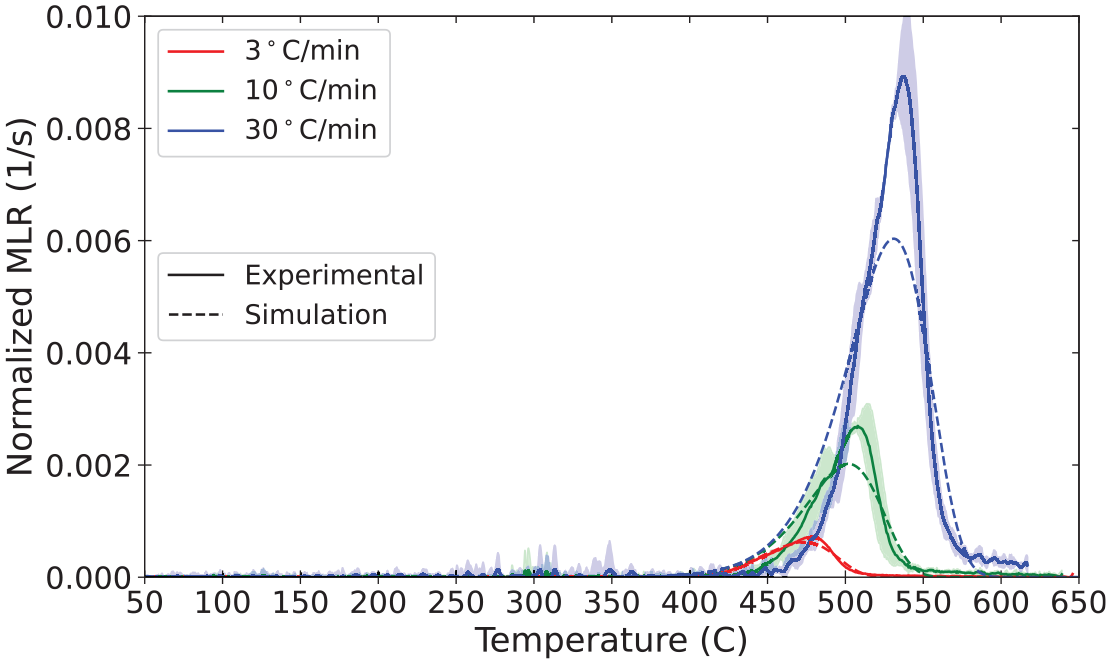
Comparison of experimental normalized MLR to model prediction for heating rates of 3°C min−1, 10°C min−1, and 30°C min−1.
STA—heat flow rate
The specific heat capacity, heat of reaction, and heat of melting determined for polycarbonate may be validated against experimental heat flow rate data collected in STA experiments. Figure 12 shows the predicted heat flow rate in a simulated STA experiment compared against the experimental data collected at heating rates of 3°C min−1, 10°C min−1, and 30°C min−1. The simulated results represented the data comparably at all heating rates. As a consequence of the shift in kinetics toward agreement with the lowest heating rate, the MLR curves showed lower magnitude peaks and wider temperature ranges which manifests in the same way in heat flow rate curves, for example the peak heat flow rate magnitudes that corresponded to the reactions are underpredicted. The agreement between the sensible enthalpy represented in the simulations and the experimental data collected provides confidence in the energetics described in the model.
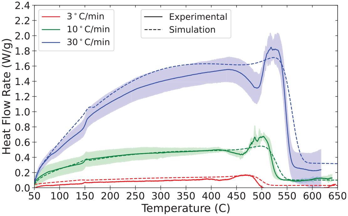
Comparison of experimental heat flow rate to model simulation for heating rates of 3°C min−1, 10°C min−1, and 30°C min−1.
CAPA
CAPA experiments were conducted in triplicate at incident heat fluxes of 25 and 75 kW m−2 on polycarbonate samples with a mean thickness of (2.41 ± 0.01) mm and a mean density of (1170 ± 10) kg m−3. The evolution of the mass and back surface temperature as well as the qualitative observations were highly repeatable across the replicate tests.
Within the first minute of exposure at each heat flux, the sample thickness was observed to increase gradually due to thermal expansion. Approximately 30 s into the tests at 25 kW m−2 and 14 s into the tests conducted at 75 kW m−2, the appearance of the sample noticeably changed from transparent to opaque white. This likely signaled the onset of decomposition with the change in visible color driven by bubble formation through the thickness of the sample. Shortly after the change in color, several large bubbles with diameters in the range of 5–15 mm emerged from the upper surface of the sample. This was followed by the formation of smaller bubbles over the entire surface of the sample and the gradual expansion of the bulk sample, forming a meniscus within the sample cup. Bubble formation became more vigorous until nearly the entire surface appeared to be boiling. This continued throughout the remainder of the test, with the material slowly turning black and extending further upward and toward the heater.
The results from the 25 kW m−2 CAPA tests on polycarbonate are shown in Figure 13 with the results of the CAPA simulation. As is shown, the MLR was low and exhibited a single peak around 500 s followed by a gradual decline. The initial nonzero MLR which decreased at the beginning of the CAPA test is an artifact of vibration of the balance due to movement of the heater in place over the sample and the transient back pressure experienced by the balance due to the high purge gas flow rate. There is no true physical mass loss that occurred at the onset of the test, and it is only noticeable because of the low magnitude MLR peak observed during the test. Due to the low MLR, there was significant noise in the measurement (MLR has been smoothed to minimize noise without affecting peak magnitude). A final residual yield of 0.88 ± 0.02 was measured in these tests. The back surface temperature shows a rapid rise until reaching a steady state at around 342°C. The relatively large aleatoric uncertainty in the temperature measurement may have been due to the loss of thermal contact between the sample and the copper foil during decomposition as well as randomness in the intumescent nature of the sample.
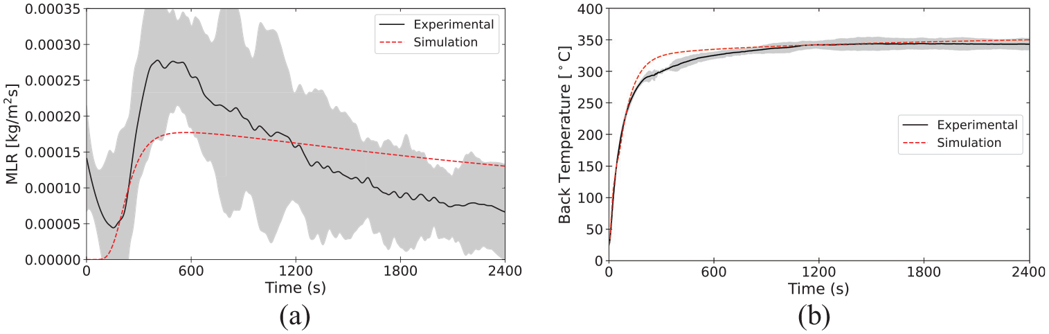
Comparison of CAPA test data to FDS simulation for polycarbonate samples below 25 kW m−2 incident heat flux: (a) area-normalized MLR and (b) back surface temperature.
The results from the 75 kW m−2 CAPA tests on polycarbonate and the corresponding model simulation are shown in Figure 14. The qualitative observations were comparable to those from the 25 kW m−2 tests albeit accelerated. A black surface char layer was formed and subsequently pushed into the center of the sample by the boiling surface. This constant accumulation led to a cone-shaped growth extended nearly 40 mm from the original sample surface which continued to grow until its base filled the entire sample cup. Representative end-test photographs of the samples are shown in Figure 15. The MLR under this heat flux exhibits different trends from those observed at 25 kW m−2. A short induction period was observed prior to the onset of significant mass loss, which was characterized by a rapid increase in MLR 25 s. This rapid increase in MLR was followed by a peak with the maximum MLR observed at approximately 100 s. From this point, the MLR sharply decreased to approximately zero by 500 s. A final residue yield of 0.17 ± 0.02 was measured in these tests. The back surface temperature showed a rapid rise until reaching a steady state at approximately 472°C. The production of pyrolyzate gases that escaped underneath the sample and obscured the optical path between the infrared camera and the back surface also led to momentary and sporadic noise in the measurements.
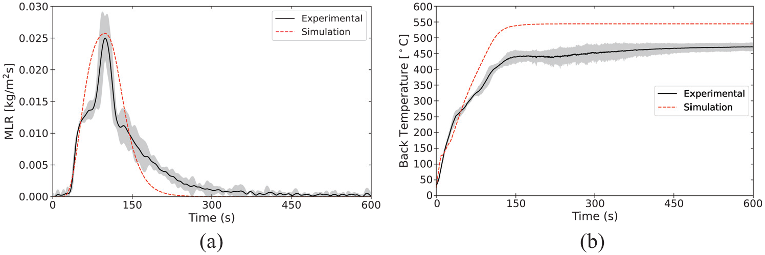
Comparison of CAPA test data to FDS simulation for polycarbonate samples below 75 kW m−2 incident heat flux: (a) area-normalized MLR and (b) back surface temperature.
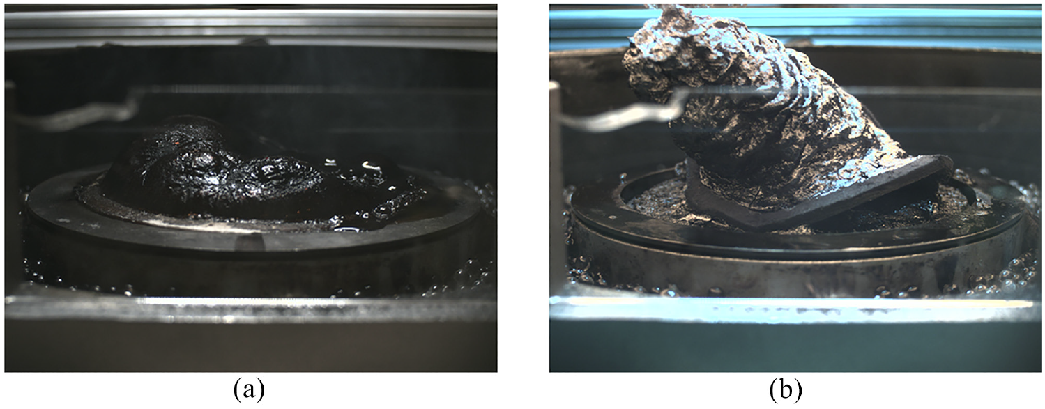
Photographs of polycarbonate samples at the end of a CAPA test: (a) 25 kW m−2 and (b) 75 kW m−2.
The agreement between the experimental CAPA data and the results of the FDS predictions are somewhat contrived because the CAPA data were used in calibration of the kinetics for the thermal degradation reaction, but the ability of the model to capture the rising edge of the MLR and back temperature data at both heat fluxes is notable and provides confidence in the properties that define the
The RMSE for the MLR data was 0.00006 kg m−2 s−1 for the 25 kW m−2 test (approximately 20% of the MLR peak magnitude) and 0.0026 kg m−2 s−1 for the 75 kW m−2 test (approximately 10% of the MLR peak magnitude). It is notable that specific features in the experimental curves which are due to complications of the thermal decomposition and gasification process for polycarbonate were not captured by the model. The model is fairly simplistic and represents the material and sample as a one-dimensional object with no explicit model representation of bubbling and associated mass transport, porosity, or the increased heat flux due to intumescence. Representation of some or all of these complicating phenomena or direct characterization of the char produced by the polycarbonate may improve agreement between the simulation and experimental data. The agreement is remarkable between the simulation and the experimental data, with the exception of the steady temperature in the 75 kW m−2 CAPA tests, given the simplicity of the model, the large difference in incident heat fluxes, and the large difference in MLR magnitude.
Cone calorimeter—piloted ignition
A phenomenon that is pertinent to fire growth and flame spread and directly applicable in fire dynamics analyses is piloted ignition given a well-characterized heat flux. The cone calorimeter is capable of generating well-defined boundary conditions, and the time to piloted ignition
The distance between the sample surface and the bottom edge of the cone heater was set to 60 mm due to the expected intumescence of the polycarbonate samples. The samples had a mean thickness of approximately 5.4 mm and a mean density of approximately 1220 kg m−3 The FDS model which simulated the cone calorimeter experiment was defined with the material properties described previously. The boundary conditions were defined such that the unexposed surface was in contact with a 25-mm-thick material with the properties of Kaowool PM board 80 which had a back face with an adiabatic boundary condition. The exposed surface of the polycarbonate sample was defined with a radiant heat flux at the boundary equal to the heat flux set point, a convection coefficient of 10 W m−2 K−1, 81 and a constant ambient temperature of 25°C. A comparison of experimental data and the simulation results are displayed in Figure 16 and are summarized in Table 17.
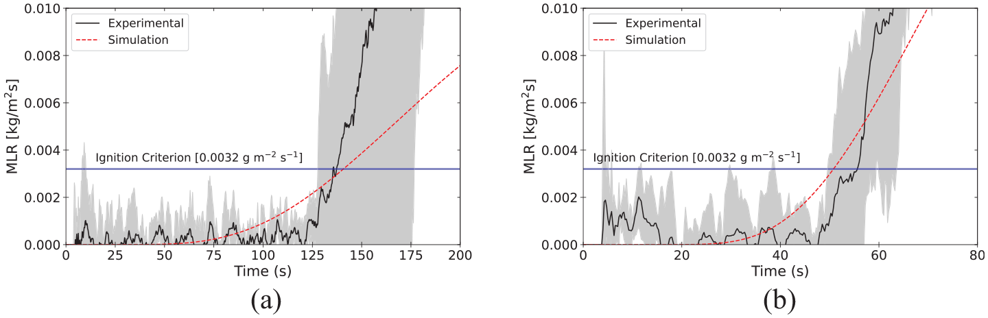
Comparison of experimental MLRPUA to model predictions for cone calorimeter tests on polycarbonate samples below 50 and 75 kW m−2incident heat flux up to ignition: (a) 50 kW m−2 and (b) 75 kW m−2.
Time to piloted ignition in cone calorimeter tests and simulations (critical mass flux = 0.0032kg m−2 s−1). Mean values presented with uncertainties represented as one standard deviation.
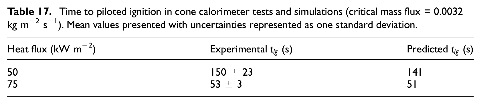
Ignition of the polycarbonate samples occurred when large bubbles at the surface of the sample burst and released flammable vapors. This mechanism which drove ignition did not always result in ignition and was not overall a highly repeatable process, so there was a lot of variation in the
Conclusion
The FSRI MaP Database fills a gap that has existed, in some form, for the fire investigation and fire modeling communities since the development of fire models. By measuring and presenting material property data on materials that are commonly encountered in the built environment, fire dynamics and risk assessment analyses may become more sophisticated, more accurate, and will result in a universally safer environment.
The experiments conducted to measure the material properties and reaction to fire in standard experiments were presented, and the major sources of uncertainty were discussed. The analytical procedures used to derive properties from experimental data were presented with example data and calculations provided for polycarbonate. A case study on validation of polycarbonate demonstrated the use of the measured and derived properties in a pyrolysis model to simulate thermal analysis experiments as well as CAPA experiments and piloted ignition in the cone calorimeter. The intention of the FSRI MaP Database is to provide data in a transparent way with all technical justification presented and to provide guidance for analytical methods to derive parameters for fire models based on the latest research. Currently, data on more than 100 materials are publicly available, and experiments are continually conducted to characterize additional materials.
Footnotes
Declaration of conflicting interests
The author(s) declared no potential conflicts of interest with respect to the research, authorship, and/or publication of this article.
Funding
The author(s) disclosed receipt of the following financial support for the research, authorship, and/or publication of this article: This work was funded in part by the National Institute of Justice (US) through grant 2019-DU-BX-0018.