Sage Journals: Discover world-class research

Abstract

Sensor-based material flow monitoring allows for continuously high output qualities, through quality management and process control. The implementation in the waste management sector, however, is inhibited by the heterogeneity of waste and throughput fluctuations. In this study, challenges and possibilities of using different types of sensors in a lightweight packaging waste sorting plant are investigated. Three external sensors have been mounted on different positions in an Austrian sorting plant: one Light Detection and Ranging (LiDAR) sensor for monitoring the volume flow and two near-infrared (NIR) sensors for measuring the pixel-based material composition and occupation density. Additionally, the data of an existing sensor-based sorter (SBS) were evaluated. To predict the newly introduced parameter material-specific occupation density (MSOD) of multi-coloured polyethylene terephthalate (PET) preconcentrate, different machine learning models were evaluated. The results indicate that using SBS data for both monitoring of throughput fluctuations caused by different bag opener settings as well as monitoring the material composition is feasible, if the pre-set teach-in is suitable. The ridge regression model based on SBS was comparable (RMSE = 3.59 px%, R² = 0.57) to the one based on NIR and LiDAR (RMSE = 3.1 px%, R² = 0.68). The demonstrated feasibility of the implementation at plant scale highlights the opportunities of sensor-based material flow monitoring for the waste management sector and paves the way towards a more circular plastics economy.

Keywords

Sensor-based material flow monitoring lightweight packaging waste plastic sorting plant machine learning prediction model near-infrared LiDAR

Introduction

In a survey conducted by the Federal Environment Agency of Austria, the operators of large sorting plants for lightweight packaging (LWP) waste in Austria confirmed that the technical potential for achieving the best sorting results has not been exploited and that there is an urgent need for modernization. Only 31–38 wt% of the output of LWP sorting plants are currently considered target fractions for mechanical or chemical recycling. The quality of polyethylene terephthalate (PET) sorting is particularly relevant in Austria, as about 25% of all plastic waste accepted for mechanical recycling in Austria is PET packaging waste. Furthermore, recyclates for food-contact applications are only allowed to be made of PET (UBA, 2021). The waste management industry faces additional pressure to improve sorting performance because of the proposal for a new regulation for packaging waste, which stipulates a recycled content of 65% by 2040 for single-use beverage bottles, which are often made of PET (EUR-Lex, 2022).

Sensor-based material flow monitoring and sensor-based quality control are already state of the art in many industries to guarantee consistently high output qualities. The food industry (Liu et al., 2017; Zeng et al., 2021) as well as the pharmaceutical industry (Botker et al., 2019) are examples of existing and precise process monitoring applications. In the field of waste management, the interest in monitoring has increased in recent years, but the technology is not yet implemented in plants (Kroell et al., 2021, 2022a). Two of the inhibiting factors are the heterogeneity of waste and the complexity of the interrelationships between different sorting stages.

One relevant factor in sorting plants, which has been investigated in the past, is high occupation density caused by high throughputs. This reduces the sorting performance of various sorting units, resulting in a reduced performance of the whole sorting plant (Kroell et al., 2022b; Kueppers et al., 2020a, 2020b). At the same time, high occupation densities inhibit the quality of sensor-based monitoring due to possible particle overlapping (Kroell et al., 2023). This leads to a special interest in determining the throughput using volume flow sensors, such as LiDAR sensors (Schwarzenbacher, 2022). Another focus is determining the material composition using sensors working in the near-infrared (NIR) range. Laboratory and pilot plant scale studies show that this enables not only the monitoring of the functionality of individual aggregates (e.g. Chen et al., 2023a; Kroell et al., 2022b; Schloegl and Kueppers, 2022) but also allows an in-line quality control and process optimization to increase the quantity and quality of PET and other target fractions (Kueppers et al., 2020a; Kroell et al., 2022a). Furthermore, the prediction of the purity at downstream measuring points is feasible in laboratory scale (Schloegl et al., 2023).

To investigate the scalability of previous studies, both additionally mounted sensors above conveyor belts (‘external sensors’) and existing sensors in sensor-based sorters (SBS) (‘internal sensors’) – using sensor fusion of data from the visible light range (VIS) and NIR – are investigated in this study. The external sensors were LiDAR sensors and NIR sensors. Due to the relevance of the PET fraction, the focus of this study is on the behaviour of the PET material in the plant. For this purpose, the feasibility of different sensors at different positions in a LWP sorting plant were investigated and based on the results, a prediction model for the PET quality of the multi-colour PET material flow was developed. In particular, the following research questions (RQ) have been investigated:

RQ1: Is it possible to monitor the effects of different bag opener settings on the throughput using LiDAR or NIR sensors?

RQ2: Can similar results concerning monitoring of throughput and composition be achieved using an existing SBS at the beginning of the sorting line?

RQ3a: Is it possible to predict PET product quality and/or quantity, based on sensor data from the beginning of the sorting plant?

RQ3b: If so, which input data and which level of smoothing are particularly beneficial?

Materials and methods

To address these research questions, multiple sensors have been installed in a LWP sorting plant in Austria. The sensor data were generated over the course of 2 weeks and exported as m³ h⁻¹ for the volume flow sensor and as classified pixels for both NIR sensors and the SBS. Furthermore, additional information concerning the plant operation was documented and included in the evaluation.

Materials

The material used for the trials was the designated input of the sorting plant. The material was not pretreated, dosed differently or otherwise manipulated in any way compared to normal plant operation. The input composition varies significantly depending on the district of origin, as there are different regulations (‘systems’) for waste separation in different regions (see Table 1). The main components in the input are bottles and other 3D objects made from PET, polyethylene (PE) or polypropylene (PP), polystyrene (PS) as well as beverage cartons (BC). Furthermore, there is 2D plastic packaging, metal packaging, other types of packaging and non-packaging waste in different shares in the mixture.

Table 1.

Examples of collection systems in Lower Austria.

Name of collection systemMaterial	910	915	930	935	Recyclabe collection
Recyclable bottles made of plastic (e.g. PET or HDPE bottles)	✓	✓	✓	✓	✓
Other plastic packaging	✓	–	✓	–	✓
Other plastics (material-equivalent non-packaging)	(✓)	–	–	–	✓
Beverage carton	✓	✓	✓	✓	✓
Other material composites	✓	–	✓	–	✓
Metal packaging	–	–	✓	✓	✓
Other packaging materials	✓	–	✓	–	✓
Other non-packaging which is suitable for recycling	–	–	–	–	✓

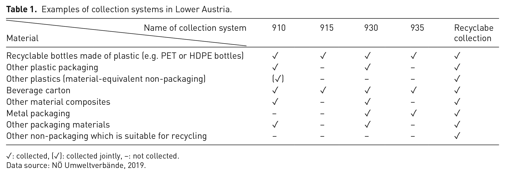
✓: collected, (✓): collected jointly, –: not collected.

Data source: NÖ Umweltverbände, 2019.

In the first phase of the trials, one truckload full of material with known origin was used as input for each trial. In the second phase, the input material was partly recently delivered and used immediately and partly material that was already stored on the property. Therefore, the documentation of the origin of the material at a certain time was not possible.

Experimental setup

The experimental setup consists of three external sensors which have been mounted over conveyor belts at different positions in the plant (see Figure 1). The first sensor (‘LiDAR’) is a volume flow sensor using LiDAR technology (Model TIM561-2050101S80; SICK AG, Waldkirch, Germany) positioned at the end of the conveyor belt of the first manual sorting station for the separation of bulky material with a belt speed of approx. 0.35 m s⁻¹. This results in an average spatial resolution of approx. 9 mm × 23 mm. The material is not singled at this point, but already lower in fluctuations of grain size through to the prior manual separation of big objects and voluminous foils. The second sensor (‘NIR1’) is also an external sensor and is mounted over the acceleration belt of the first SBS unit in the plant, together with the corresponding halogen lights. This SBS unit is positioned directly after the ballistic separator in the 3D stream. The measured belt width is 1.99 m, and the belt speed is approx. 2.7 m s⁻¹ and presented as a singled monolayer to the SBS unit. This sensor is a NIR sensor (Model G2-320; EVK DI Kerschhaggl GmbH, Raaba, Austria) with a spectral resolution of 212 px (≙3.1 nm per band), a spatial resolution of 312 px and operated at a framerate of 300 Hz. The third measuring point (‘SBS’) is the before mentioned SBS (Unisort PC 2000 R, RTT Steinert GmbH, Köln, Germany), which exports a data stream of fusioned data from the internal NIR and a VIS sensors. The fourth sensor (‘NIR2’) is another external NIR sensor of the same model and settings as described before. It is positioned after multiple sorting steps over the acceleration belt of another SBS to create a PET stream. Again, a high material singulation, meaning almost no particles touching or overlapping according to Kroell at al. (2024), is observed at a belt speed of approx. 1.1 m s⁻¹. The belt width is 1.80 m and therefore slightly smaller than at NIR1.

Figure 1.

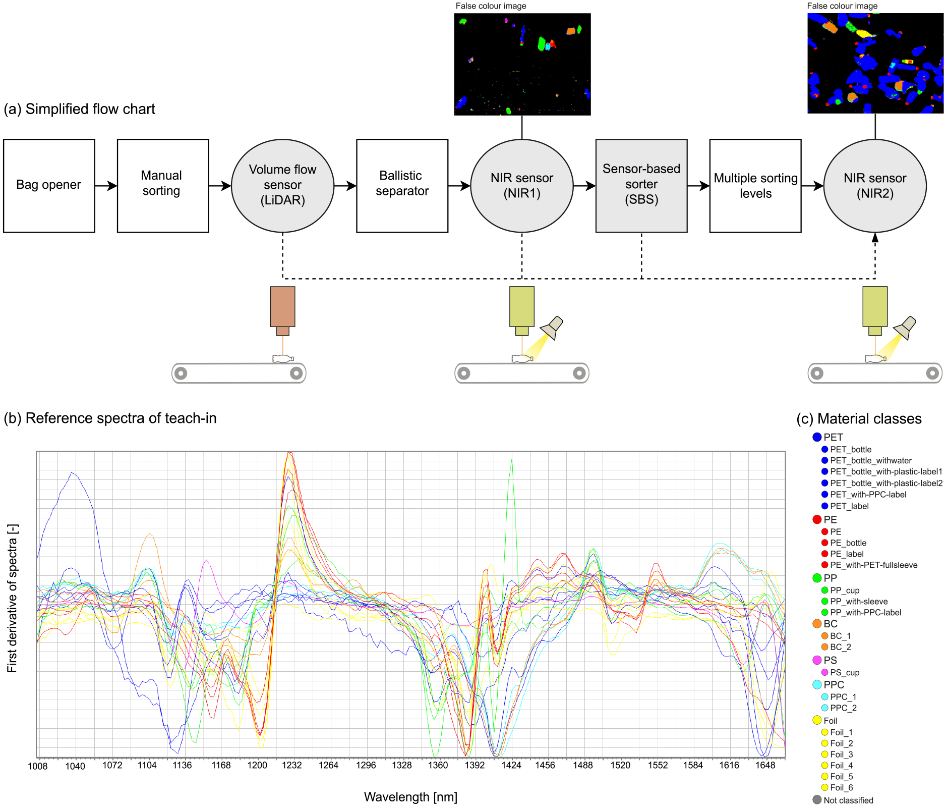
Experimental setup for material flow monitoring: (a) simplified flow chart of sorting plant including internal and external sensors (grey). False colour image of NIR1 and NIR2 during plant operation; (b) corresponding reference spectra and chosen material classes of teach-in.

Installation and setup of external sensors

For reliable data acquisition, the external sensors were conscientiously prepared individually. The LiDAR sensor was calibrated after the installation to enable the conversion of the measured signal into metric units [m³ s⁻¹]. For both external NIR sensors, a teach-in including the most relevant plastic packaging materials was created manually (see Figure 1(b)). For this purpose, representative pixels were selected from the raw data images of conscientiously chosen reference particles. The pre-processed NIR spectra (first derivative, normalized, smoothed) of each of these pixels thus result in an average spectrum. Several of such average spectra can be combined into one material class. For example, it was defined that both PET bottles and labels on PET bottles should be classified as ‘PET’, to reduce the influence of labels on the NIR classification (cf. Chen et al., 2023b, Schloegl et al., 2022). Particular attention was devoted to ensuring that the teach-ins for NIR1 and NIR2 produced results as similar as possible to enable comparability of the data.

In Table 2, a list of the resulting material classes of the created teach-ins for NIR1 and NIR2 is presented together with the list of material classes of the existing SBS. PET, PE, PP, PS and BC are material classes in both lists. It is important to consider that the chosen reference materials from the manufacturer of the machinery as well as the classification algorithm and other factors like frame rate and spatial and spectral resolution differ between the external and internal NIR sensors. Therefore, the total number of pixels of an identical object will be different at NIR1 and SBS.

Table 2.

Comparison of material classes of the external sensors (NIR1 and NIR2) and the internal sensor of the sensor-based sorter (SBS).

Material class	Material	NIR1 and NIR2	SBS (NIR + VIS)
PET	Polyethylene terephthalate	✓	Sub-classes: clear, blue, green, other colours, blisters
PP	Polypropylene	✓	✓
PE	Polyethylene	✓	✓
PS	Polystyrene	✓	✓
BC	Beverage carton	✓	✓
PPC	Paper, paperboard, cardboard	✓	–
Foils	Mainly PE films	✓	–
NC	Not classified	✓	–
PVC	Polyvinyl chloride	–	✓
Cellulose		–	✓
Others		–	✓

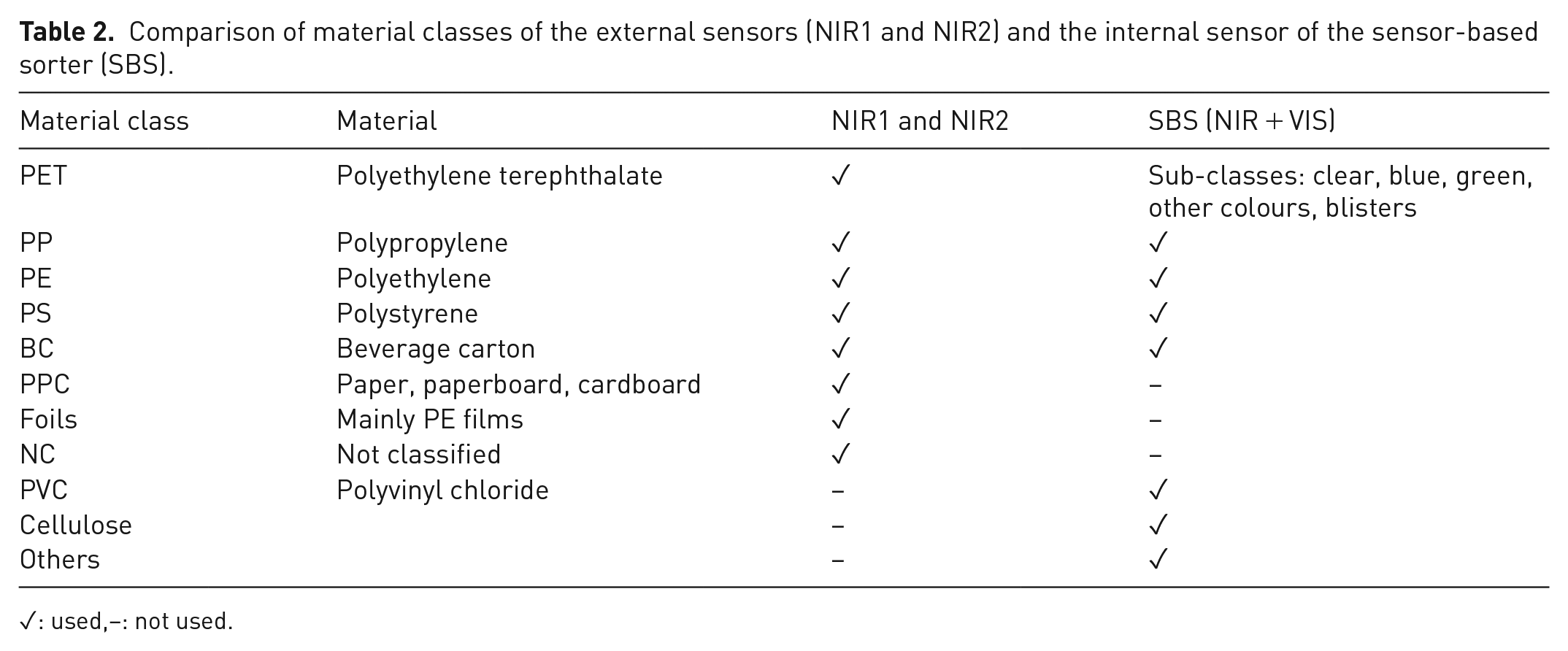
✓: used,–: not used.

Experimental procedure

The data acquisition was divided in two phases. In both phases, the settings of the bag opener have been documented. The rotation speed of the bag opener was set by selecting a number between 12 and 20. Setting 12 represents 3–4 rpm, whereas setting 20 represents 7 rpm. Further settings investigated during the trials are 16 (5 rpm), 17 (6 rpm) and 18 (6 rpm).

In the first phase, the chosen bag opener settings were 12, 16 and 20. In this phase, only material of one truckload at a time with known origin and weighted mass (between 6.8 and 8.1 t per truck load) was fed into the bag opener. This was done four times with varying order of the three settings. As the external NIR sensor data were not available for that time period, only LiDAR and SBS data were investigated.

In the second phase, there was no interference with the plant operation at all. Therefore, the dominating settings in that time were 17 and 18. Of the total of 10 trial days, only at 4 days both the NIR1 and NIR2 data were available in addition to LiDAR and SBS data due to an unfortunate loss of data.

To enable the correlation of different measurement points, the transport times have been measured. To do this, material was fed into the emptied plant. One person was waiting at each measurement point and screenshotting the time of an online atomic clock at the exact moment the first material passed. The resulting average transport times are as follows: Input-LiDAR: 69 s, LiDAR-NIR1/SBS: 29 s and NIR1-NIR2: 77 s. The SBS had a shift in time of about 100 s compared to NIR1, as it is apparently not aligned with an atomic clock.

Statistical evaluation

Different data preparation steps were required for the different data sets. The data of the LiDAR sensor (maximum height and volume flow in m³ s⁻¹) have a frequency of 15 fps, these were aggregated to 1 s, 5 s, 1 minute and 5 minutes values and converted to m³ h⁻¹ for the visualization. The SBS data are given as 1 minute values and were aggregated to 5 minutes values in an additional data set. For NIR1 and NIR2, 10 values per second are given on average. They number of pixels per material class (e.g. PET) were aggregated to 1 s. The material-specific occupation density (MSOD) (see equation (2)) is calculated based on the 1 s values. The resulting 5 s, 1 minute and 5 minutes values of MSOD were calculated by using the average of 1 s values.

To exclude the data recorded during plant downtime, the LiDAR data with a time resolution of 5 s were used. The relevant criteria was constant phases of maximum height and volume flow in m³ s⁻¹, thus the previous or following 7 values (≙35 s) staying within the current value ± 3.3% of the value range. For the aggregation of on–off values from 5 s to 1 minute and 5 minutes, the median in an interval was used (majority vote on or off). Based on this data, the NIR and SBS data were also filtered accordingly. Therefore, only data where the described method based on LiDAR data did not detect a stop were used in the following analysis.

The number of sorting personal for 2D and 3D was recorded in lists, typically per 8 hours shift, or more granular if changes happened during a shift. The records are then mapped to the 5 s, 1 minute and 5 minutes data points at NIR1 timing.

The NIR and SBS data presented in this study are given as occupation density (pixel share of material on the conveyor belt) or MSOD (share of one material on the conveyor belt; see equation (1)), which is introduced by us. The benefit of this parameter compared to the common use of material shares (see equation (2)) is that MSOD combines the information of pixel-based material shares (c_a) and occupation density (OD). MSOD can be calculated by multiplying both values (see equation (3)).

c_{a, PET} = \frac{{pixels}_{PET}}{\sum_{i} {pixels}_{material < i >}} = \frac{a_{PET}}{\sum_{i} a_{material < i >}}

(1)

{MSOD}_{PET} = \frac{{pixels}_{PET}}{\sum_{i} {pixels}_{< i >}} = \frac{a_{PET}}{a_{total}}

(2)

{MSOD}_{PET} = c_{a, PET} * OD

(3)

The total amount of data for LiDAR and SBS is 9, 608 minutes, which is approximately 160 hours. The selection of data used to visualize the correlation of throughput and occupation density at bag opener settings 12-16-20 each cover approximately 90 minutes and therefore about 4.5 hours in total. For the ridge regression model, about 31 hours of training data (80%) and 7.5 hours of test data (20%) was used.

For the visualization of correlation plots the data within the 99.5 percentile is presented. The reason for excluding extreme outliers is to improve readability for the majority of the data. For improved visualization of the violin plots, extreme outliers were excluded. In addition to filtering plant stops, values below 12.6 m³ hour⁻¹ for LiDAR and below 0.46 px% for SBS were excluded. All other outliers, especially those above the median, are visible as dots in the plot.

Results and discussion

The presented results are structured according to the research questions presented in section ‘Introduction’, regarding monitoring the effects of different bag opener settings (RQ1), the exploitability of SBS data at the beginning of a sorting line (RQ2) and creating a prediction model for the PET material flow (RQ3a, b).

Correlation of LiDAR and SBS data

The results presented in Figure 2 show a general dependency of chosen settings of bag opener and resulting throughput. The data of 2 days, in which all settings occurred, are visualized as violin plots (Figure 2(a) and (b)). Low rotation speeds (bale opener settings 12 ≙ 3–4 rpm) result on average in lower measured volume flows. The median volume flow at setting 20 (≙7 rpm) is 1.94 times higher than at setting 12. The distribution of values within a setting does not correspond to a Gaussian distribution. This is likely caused by fluctuations of input composition, fluctuations of input feed and fluctuations in residence time of different materials in the bag opener. The corresponding plots of occupation density measured by the SBS (transport time from LiDAR 29 s) show in general similar results. The exception occurs at setting 17 (≙6 rpm) where the median is lower than setting 16 (≙5 rpm) and differs from setting 18 although the rotation speed is in a similar range (≙6 rpm). Since the scatter of the values at 17 and 18 is greater than for other values, it is reasonable to assume that the material-specific behaviour in the bag opener influences the resulting grain size distribution as well as the material at the conveyor belt.

Figure 2.

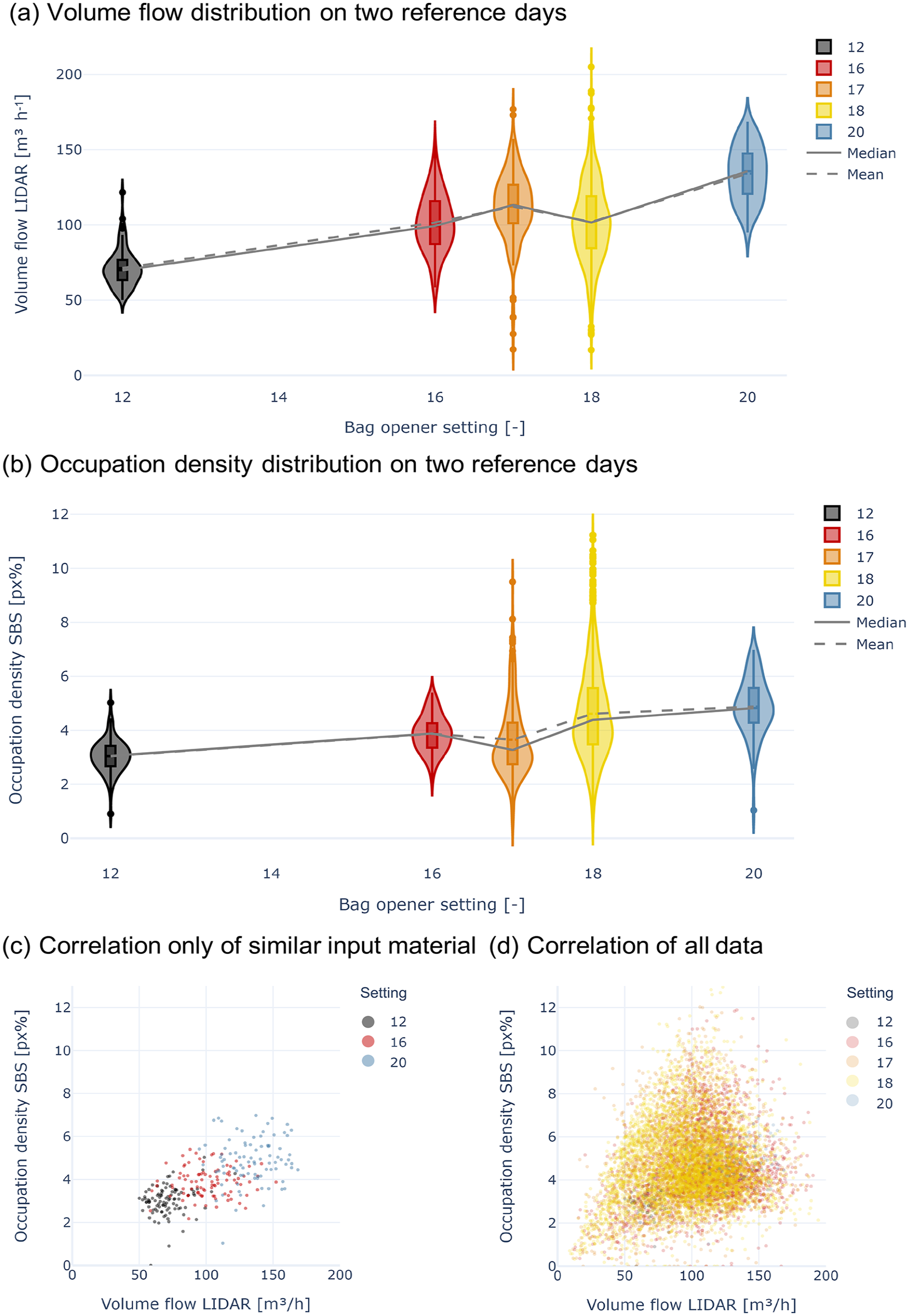
Correlation of LiDAR and SBS data at different bag opener settings. (a) Volume flow on two reference days. (b) Occupation density on two reference days. (c) Correlation of similar input material. (d) Correlation of all data. Colour code of settings: black: 12 ≙ 3–4 rpm, red: 16 ≙ 5 rpm, orange: 17 ≙ 6 rpm, yellow: 18 ≙ 6 rpm, blue: 20 ≙ 7 rpm.

In Figure 2(c) and (d), the correlation of volume flow and occupation density is presented. One point in the graphs represents 1 minute of data. As the volume flow increases, the occupied area on the belt increases; thus, the pixel-based occupation density. One reason for the dispersion of values is the fact, that the ballistic separator is positioned between the LiDAR sensor and SBS. As the sorting performance of a ballistic separator depends on the throughput, the resulting material flow (throughput and composition) at the SBS is not constant with different bag opener settings. In Figure 2(c), only results for input material of known origin is presented. By doing so, the effects of different bag opener settings for similar input material are visible. When plotting all data (see Figure 2(d)), the influence of the bag opener setting is not visible anymore. This range of results is again caused by fluctuations of input composition, fluctuations of input feed, fluctuations in residence time of different materials in the bag opener and the effects of the ballistic separator. Thus, no conclusive and generally applicable correlation formula between LiDAR and SBS data can be derived from the data. Nevertheless, there is an evident correlation within the same material. Therefore, the monitoring of variations within the same input material seems to be possible not only by using an external LiDAR sensor but also with existing internal sensors of the SBS.

Correlation of NIR1 and SBS data

To investigate the feasibility of using SBS for monitoring the material flow composition, the MSOD data of NIR1 and SBS are correlated in Figure 3. The data basis is 2291 of 1 minute values equivalent to about 38 hours. The results show differing behaviour for different materials. PET showed the most similar results due to the almost perfect alignment between the MSOD of internal and external NIR sensors (blue diagonal in the plots). For PET, PE and PP, the SBS data are higher on average, whereas for PPC and PS, the SBS is lower than die NIR1 data. BC shows an overestimation of lower values, whereas for NIR1-MSOD, values higher than 0.5, the corresponding SBS values are underestimated. The best coefficient of determination (R²) is achieved for PET (R² = 0.69), the worst for PS (R² = 0.14). The good results for PET are most likely due to the fact that the SBS ejects PET; therefore, this material class must have had a high priority for the manufacturer when creating the internal teach-in of the SBS unit.

Figure 3.

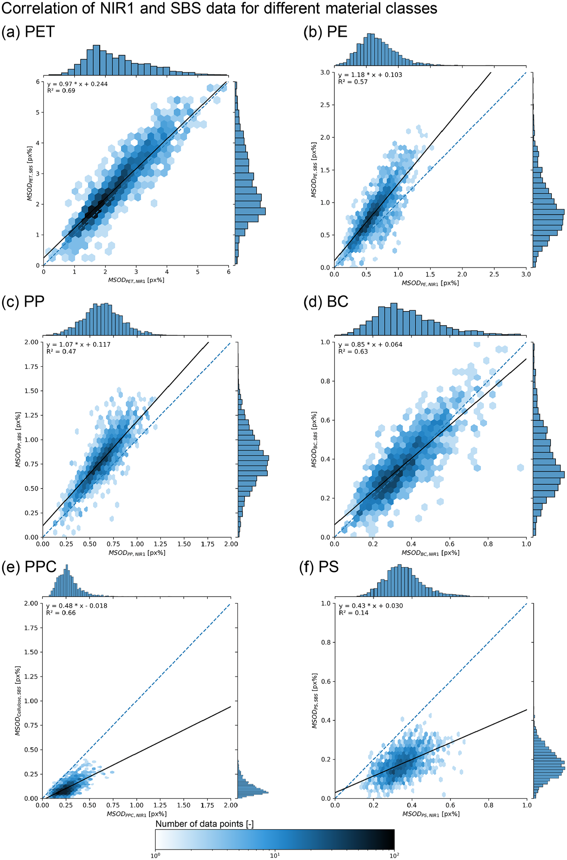
Correlation of NIR1 and SBS MSOD data presented as hexbin plots including frequency distribution and fit function for different materials: (a) PET, (b) PE, (c) PP, (d) BC, (e) PPC and (f) PS. Presented data: 1 minute values, reduced to 99.5 percentile of all values; Heatmap based on a logarithmic scale; Blue diagonal represents perfect correlation of the data; Non-equal axis to improve legibility; MSOD: material-specific occupation density.

Since PE and PP are also materials commonly found in PET bottles – mainly as caps, sometimes also in the form of labels – these were also prioritized and possibly even weighted when creating the internal teach-in of the SBS unit. Detailed information about the teach-in from the manufacturer was not provided upon request. This is a fundamental problem when using data from existing SBS units. Through the temporary use of an external sensor with a known teach-in, conclusions can be drawn about the otherwise inaccessible teach-in of the SBS.

Prediction model

Various types of models were tested in preliminary studies for their suitability in predicting the PET stream at the end of the plant. For using a deep learning model, the number of available data points was not sufficient. The models tested more detailed and compared by root mean squared error (RMSE) included random forest (RMSE = 3.47 px%) and linear regression (RMSE = 3.11%). Ridge regression performed slightly better than linear regression and was therefore investigated further.

An occurring issue when using sensors that allow high temporal resolution is which degree of aggregation is suitable for practical use (cf. Kroell et al., 2023). If there are many data points per second, a lot of information is available, but within the data points there are high fluctuations. With too much smoothing, however, too much information is lost. Therefore, Figure 4 shows the comparison of the actually measured data (‘Test’, black) and the values predicted according to the ridge regression model (‘Pred’, blue) for different levels of data smoothing. The ridge regression model was used with regularization parameter α = 1 and exhibited better performance than compared linear regression and random forest models. Neural network models were also tested but did not perform that well, most likely to the limited amount of data recorded – for larger observation periods they might be a good choice.

Figure 4.

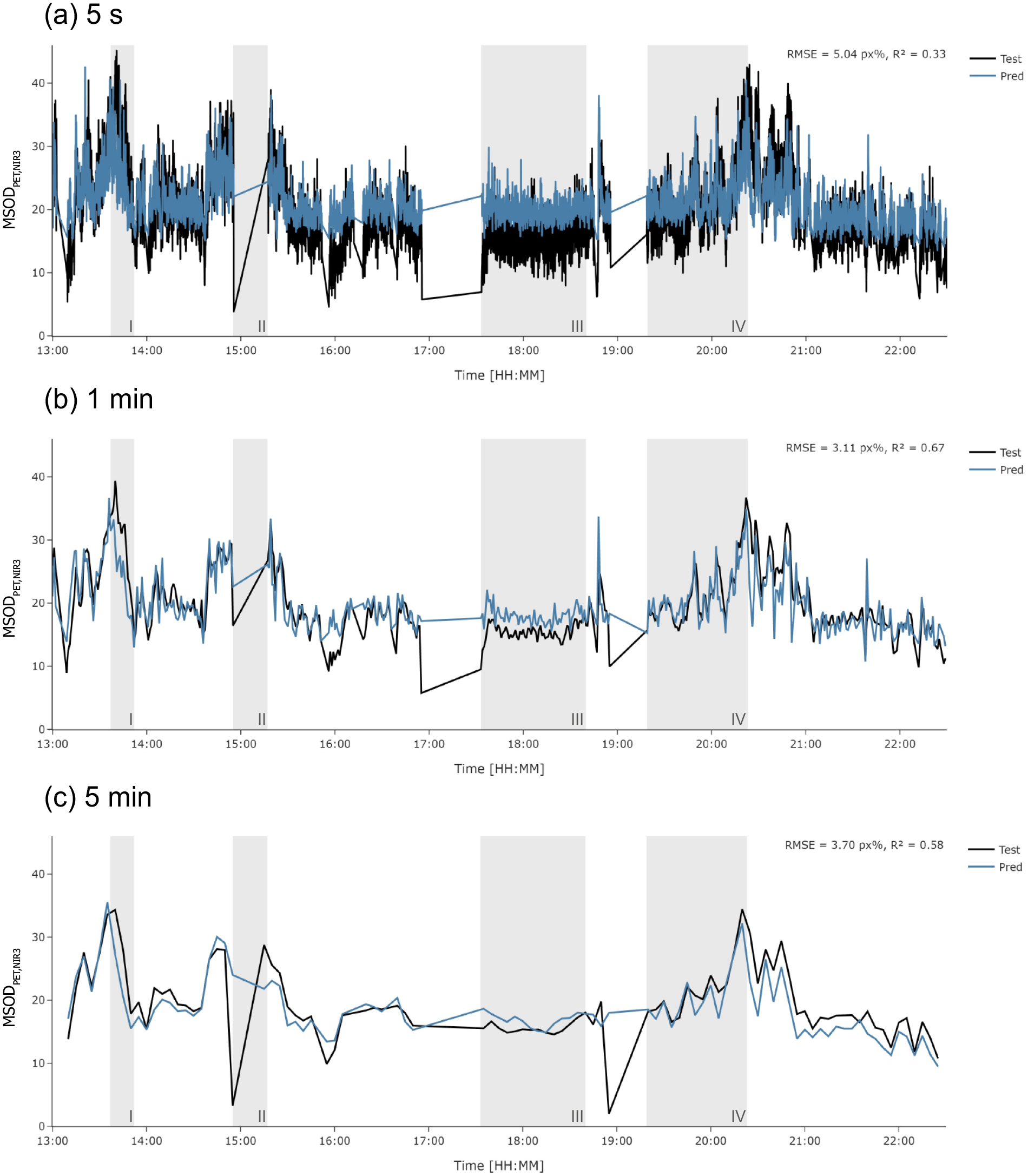
Time series graph of prediction model for MSOD_PET at NIR2 based on NIR1 data using ridge regression for different levels of data smoothing: (a) 5 s, (b) 1 minute, (c) 5 minutes. Black: Test data, Blue: Prediction. Areas highlighted in grey: (I) Underestimation, (II) Plant shutdown during break – Overestimation, (III) Overestimation, (IV) Similar results; MSOD: material-specific occupation density.

The best results with respect to coefficient of determination (R² = 0.67) and RMSE = 3.11 px% are for 1 minute smoothing. In general, it is difficult to achieve lower values for R² in waste sorting plants, due to the high heterogeneity. The demands on accuracy are, therefore, lower than, for example, in the food or pharmaceutical industry. It is important to emphasize that the best results at 1 minute smoothing may be due to the limited amount of data available. The 31 hours of training and 7.5 hours of test data correspond to only 408 training and 93 test samples at 5 minutes smoothing. If the data were recorded over a year instead of 10 days, the error values for the 5 minutes smoothing would most likely be better.

Regardless of the degree of smoothing, the trends of the test and prediction data are similar. The afternoon breaks, daily at 15:00 (II), 17:00 and 19:00 are visible in all diagrams. Furthermore, overestimation (III) or underestimation (I) occurs in similar time slots for different levels of data smooting. There is a tendency for low MSOD test data values resulting in overestimation, whereas higher MSOD test data values result in underestimation. Area IV shows particularly similar results of test data and prediction in all diagrams. It can be concluded that even a less favourable selection of the smoothing does not necessarily lead to problems in monitoring.

From the data presented in section ‘Statistical evaluation’, the hypothesis can be derived that the prediction of the PET flow at measurement point NIR3 based on the SBS data should work similarly as the prediction based on NIR1. This hypothesis is confirmed when looking at the hexbin plots in Figure 5(a). In the top two plots, LiDAR data were also included in the training process to investigate whether this would improve the prediction model. The comparison to the plots without using the LiDAR data shows no benefit. The use of MSOD – which indirectly covers the throughput by using the occupation density – seems to make the LiDAR obsolete for this application. The comparison of the RMSE values and R² score for the different models shows the best results for NIR1 + LiDAR (R² = 0.68, RMSE = 3.10 px%), followed by NIR1 (R² = 0.67), SBS (R² = 0.57) and SBS + LiDAR (R² = 0.54, RMSE = 3.72 px%). The same ranking of the models is obtained when evaluating the width of the 95% prediction interval, which was always around double the RSME value.

Figure 5.

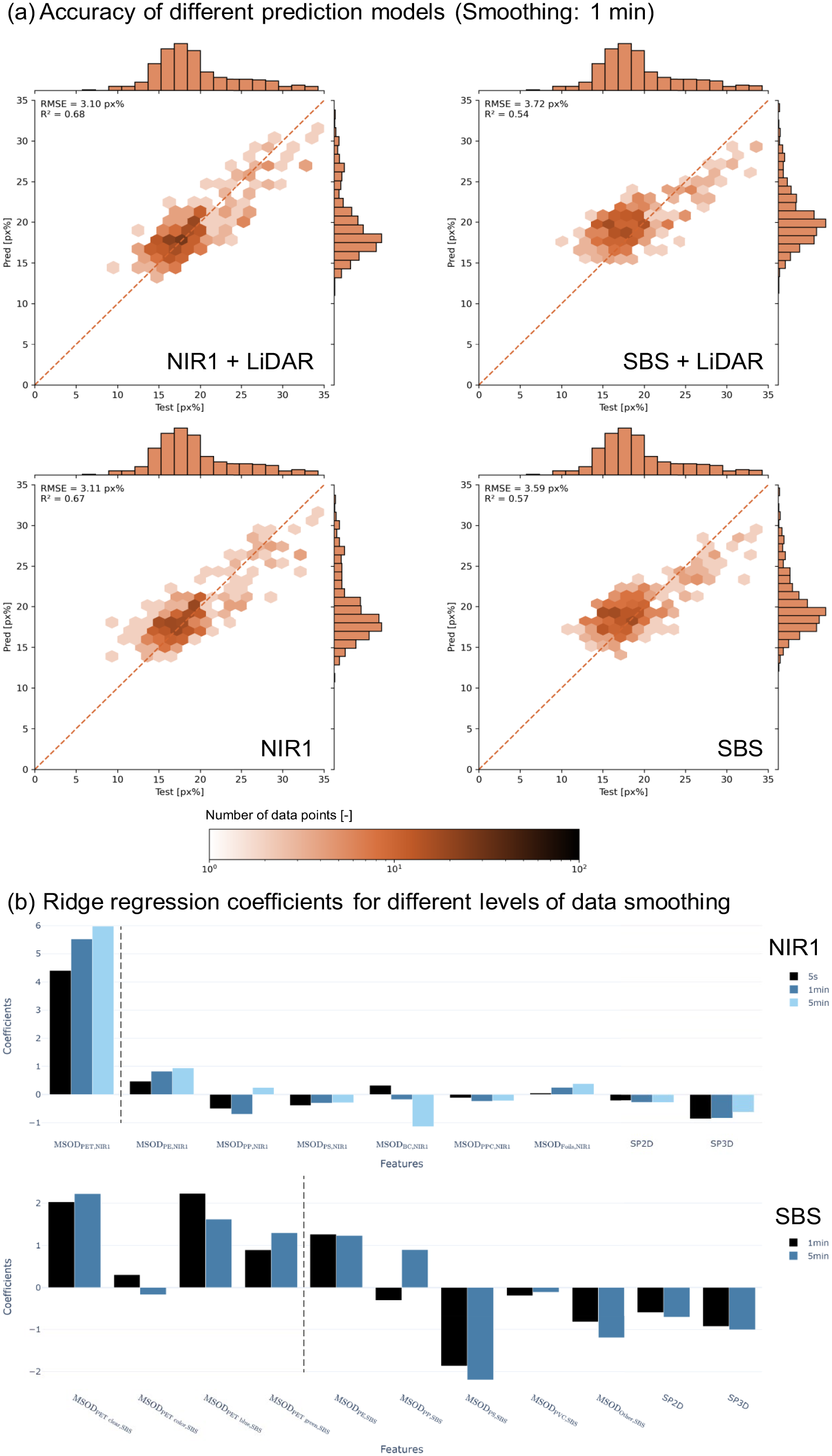
Ridge regression prediction model: (a) comparison of different combinations of input data (NIR1/SBS, LiDAR, number of personnel) presented as hexbin plots including perfect correlation (orange diagonal), R² and RMSE values. (b) Coefficients of ridge regression based on NIR1 and SBS data (without LiDAR) for different levels of smoothing; MSOD: material-specific occupation density.

In all cases, the number of sorting personal was also considered as an input feature, increasing model accuracy, even though only a very limited number of shifts with different personal setup was observed. However, explaining the influence of these parameters proved to be difficult. It is negative at first sight (see Figure 5(b): ‘SP2D’ and ‘SP3D’), although we would expect it to be positive. More detailed analysis showed that the number of personal seem to act as a proxy for night shifts, where more personal was present during the recording of experimental data. Extracting the night shift as a separate parameter shows positive influence of sorting personal count, with larger negative influence of night shift (vs day shift).

The most relevant features of the ridge regression models of NIR1 and SBS (without LiDAR) are presented in Figure 5(b) by comparing the linear coefficients. Comparability is given due to the application of a standard scaler before training the models. For both models, the most important feature is the MSOD of PET. Since the SBS has different colour categories for PET due to the VIS sensor, it can additionally be deduced that PET clear and blue are the most important colours. However, this could simply be because these colours occur most frequently in PET bottles. For both models, the coefficient of PE is positive and of PS is negative. For PP, the coefficient is negative for lower levels of smoothing and positive for the highest level of smoothing. As stated before, for both models, the number of people in the manual sorting stations for 2D (‘SP2D’) and 3D (‘SP3D’) material have negative coefficients.

Conclusion

To meet the target quotas for recycling, sorting plants urgently need to exploit their technical potential. One important tool for this is sensor-based material flow monitoring. Since past studies have shown that throughput fluctuations affect the quality of output fractions, the effects of different bag opener settings were investigated. To do so, different types of sensors at the beginning of the plant were investigated (RQ1). As mounting external sensors can be cost-intensive, the results were further compared to the results based on data of existing sensors within a SBS (RQ2).

It was found that the resulting volume flow is not linearly related to the settings of the bag opener. In at least one area of the relation, an increased bag opener setting can even lead to a decreased volume flow. Nevertheless, when comparing the extreme values of setting 12 and setting 20, an increase in throughput is measurable. The comparison of the resulting volume flow (LiDAR) and the occupation density of SBS indicates that although there is a spread in the results, using SBS data is sufficient for a general estimation of the plant throughput.

The comparison of the first external NIR and SBS data taken at the same position in the plant showed an even better correlation. When using SBS data, there is a risk that the requirements for the sorting task, and the material flow monitoring do not match. In the present study, there happened to be a good correlation with respect to PET. However, the correlation is material dependent – the worst correlation was with PS. This means that usually the SBS monitors materials well it was targeted for, whereas an external NIR sensor gives a more complete picture of the material flow. For real-life implementations, the monitoring results of SBS data could possibly be improved by adapting the teach-in, if machine manufacturers allow access. A possible solution that would not impair the sorting result could be separate data processing for the two applications (sorting and monitoring). However, if either access to the data is not available or no SBS is positioned at a relevant position in the plant, external NIR sensors provide a reliable data source for monitoring.

Based on the assessment of all available sensor data, different machine learning models for the prediction of the material flow at the end of the plant based on data at the beginning of the plant were evaluated. The aim was to predict the quality of the multi-coloured PET stream, due to the relevance of the PET fraction for recycling (RQ3a). A new parameter was introduced for this purpose: MSOD (px%). This value results from multiplying pixel-based material share and occupation density. Thus, the composition and the throughput can be expressed simultaneously.

When comparing the types of models in preliminary studies, ridge regression emerged as the best model. This model was further tested for smoothing at different levels (RQ3b), whereby the 1 minute values appeared to be the best. However, the theory is that this is also due to the limited duration of the experiment (about 38.5 hours of data during plant operation). If monitored over the course of a year, the 5 minutes values could give better results, but it could also be that capturing faster changes in the material flow and sorting process keep the 1 minute average as the best alternative. The comparison of the different input feature sets from the sensors (NIR1/SBS plus optional LiDAR) found that using the LiDAR data had no positive effect. When comparing NIR1 and SBS data only, NIR achieved better results (RMSE = 3.11 px%, R² = 0.67). Nevertheless, SBS data are also suitable (RSME = 3.59 px%, R² = 0.57) as in many applications there is a broader tolerance range, due to the high heterogeneity of waste.

In all cases, the number of sorting personal was also considered as an input feature, increasing model accuracy, even though only a very limited number of shifts with different personal setup was observed. Although an improvement in the PET stream would be expected with increasing numbers of people, the regression model coefficient was negative. More detailed analysis revealed that there were more people on night shifts. When comparing day shift to night shift, the coefficient was positive for the day and negative for the night. Therefore, sorting personal showed interesting challenges in feature selection.

In conclusion, it can be said that a model for predicting the material flow rather at the end of the plant based on data rather at the beginning of the plant has been successfully made. There is a great potential for the use of such a model, from the use directly in the plant operation to the modelling of different scenarios to determine the ideal conditions for an economic, as well as ecological operation. For commercial implementation, it is necessary to apply monitoring on a long-term basis in a plant for a comprehensive investigation of the resilience of the model.

Footnotes

Declaration of conflicting interests

The authors declared no potential conflicts of interest with respect to the research, authorship, and/or publication of this article.

Funding

The authors disclosed receipt of the following financial support for the research, authorship, and/or publication of this article: We would like to thank the individuals and companies who helped with the planning and execution of the experiments. A special thanks go to the team of student workers: Georg Schmölzer, Alexander Weber and Sebastian Wilhelm. Moreover, we thank our project partners for providing equipment and support. In particular, the team of Brantner Sort4you GmbH, Bastian Küppers and Elias Pfund and the rest of the team of Stadler Anlagenbau GmbH, the team of EVK DI Kerschhaggl GmbH, as well as the team of Siemens AG Austria. Further Sebastian Frank (Siemens Advanta Solutions GmbH) for his input. Finally, we would like to thank the Austrian Research Promotion Agency for funding the project ‘EsKorte’ within the programme ‘Production of the Future’ under grant agreement 877341.

ORCID iDs

Sabine Schloegl

Nils Kroell

Daniel Vollprecht

References

Botker

Rantanen

(2019) Chapter 3.7 – Hyperspectral imaging as a part of pharmaceutical product design. Data Handling in Science and Technology 43: 567–582.

Chen

Kroell

Hofmann

, et al. (2023a) Improving drum sieve performance in lightweight packaging waste recycling by automatic parameter adjustment through 3D laser triangulation-based process monitoring. Resources, Conservation and Recycling 192: 106924.

Chen

Kroell

Althaus

, et al. (2023b) Enabling mechanical recycling of plastic bottles with shrink sleeves through near-infrared spectroscopy and machine learning algorithms. Resources, Conservation and Recycling 188: 106719.

EUR-Lex (2022) Regulation of the European Parliament and of the Council on packaging and packaging waste, amending Regulation (EU) 2019/1020 and Directive (EU) 2019/904, and repealing Directive 94/62/EC (Text with EEA relevance). Document 52022PC0677. Brussels, 30.11.2022. Available at: https://eur-lex.europa.eu/legal-content/EN/TXT/?uri=CELEX:52022PC0677&qid=1677599742471

Kroell

Chen

Maghmoumi

, et al. (2021) Sensor-based particle mass prediction of lightweight packaging waste using machine learning algorithms. Waste Management 136: 253–265.

Kroell

Chen

Greiff

, et al. (2022a) Optical sensors and machine learning algorithms in sensor-based material flow characterization for mechanical recycling processes: A systematic literature review. Waste Management 149: 259–290.

Kroell

Dietl

Maghmoumi

, et al. (2022b) Assessment of sensor-based sorting performance for lightweight packaging waste through sensor-based material flow monitoring: Concept and preliminary results. In: Proceedings of 9th sensor-based sorting and control 2022, Aachen, Germany, 13–14 April 2022.

Kroell

Chen

Küppers

, et al. (2023) Near-infrared-based determination of mass-based material flow compositions in mechanical recycling of post-consumer plastics: Technical feasibility enables novel applications. Resources, Conservation and Recycling 191: 106873.

Kroell

Maghmoumi

Dietl

, et al. (2024) Towards digital twins of waste sorting plants: Developing data-driven process models of industrial-scale sensor-based sorting units by combining machine learning with near-infrared-based process monitoring. Resources, Conservation and Recycling 200: 107257.

10.

Kueppers

Seidler

Koinig

, et al. (2020a). Influence of throughput rate and input composition on sensor-based sorting efficiency. Detritus 9: 59–67.

11.

Kueppers

Schloegl

Friedrich

, et al. (2020b) Influence of material alterations and machine impairment on throughput related sensor-based sorting performance. Waste Management & Research 39: 122–129.

12.

Liu

Hongbin

Dawen

(2017) Hyperspectral imaging technique for evaluating food quality and safety during various processes: A review of recent applications. Trends in Food Science & Technology 69: 25–35.

13.

NÖ Umweltverbände (2019) Niederösterreichische Restmüllanalyse 2018/2019 (Lower Austrian residual waste analysis 2018/2019). Available at: http://www.noe.gv.at/noe/abfall/noe_restmuellanalyse_2018_2019.pdf

14.

Schloegl

Kueppers

(2022) Quantifying the delabelling performance using sensor-based material flow monitoring. In: Proceedings of 9th sensor-based sorting and control 2022, Aachen, Germany, 13–14 April 2020.

15.

Schloegl

Schmoelzer

Weber

, et al. (2023) Monitoring the sorting performance in lightweight packaging waste sorting plants using data of sensor-based sorters. In: Proceedings of international conference on optical characterization of materials (OCM 2023), Karlsruhe, Germany, 22–23 March 2023.

16.

Schwarzenbacher

(2022) Quantitative beurteilung der LiDAR-technologie zur volumetrischen stoffstromcharakterisierung von material (Quantitative evaluation of LiDAR technology for volumetric material flow characterization of material). Master’s thesis, Montanuniversität Leoben. Available at: https://pure.unileoben.ac.at/portal/files/8829840/ac16509071.pdf

17.

UBA (2021) Sortierung und recycling von Kunststoffabfällen in Österreich: Status 2019 (Sorting and recycling of plastic waste in Austria: status 2019). 2nd edn. Federal Environmental Agency of Austria (UBA). Report rep-0744. Viena 2021.

18.

Zeng

Guo

Han

, et al. (2021) A review of the discriminant analysis methods for food quality based on near-infrared spectroscopy and pattern recognition. Molecules 26: 749.

Developing a prediction model in a lightweight packaging waste sorting plant using sensor-based sorting data combined with data of external near-infrared and LiDAR sensors

Abstract

Keywords

Introduction

Materials and methods

Materials

Experimental setup

Installation and setup of external sensors

Experimental procedure

Statistical evaluation

Results and discussion

Correlation of LiDAR and SBS data

Correlation of NIR1 and SBS data

Prediction model

Conclusion

Footnotes

Declaration of conflicting interests

Funding

ORCID iDs

References