
Abstract
Lidar-based simultaneous localization and mapping (SLAM) enables the generation of detailed 3D maps for such applications as autonomous navigation and infrastructure monitoring. However, SLAM systems are prone to drift accumulation, especially in the absence of a tightly integrated global navigation satellite system (GNSS) or inertial measurement unit, leading to degraded global accuracy. This paper presents a modular, post-processing correction pipeline that leverages high-accuracy GNSS real-time kinematic (RTK) data to correct lidar SLAM outputs in high-drift scenarios. The pipeline operates in three stages: (1) segment-based SLAM trajectory correction through alignment with time-synchronized GNSS RTK points using a singular value decomposition and Iterative Closest Point (SVD-ICP) method; (2) propagation of these corrections to the aggregated point cloud through timestamp-aligned delta application, generating a non-rigid intermediate reference map; and (3) conditional map refinement using either the SVD-ICP method for globally rigid alignment in low-drift scenarios or a Random Sample Consensus (RANSAC)-progressive Iterative Closest Point (ICP) method for robust registration in cases with significant residual drift, outliers, or local inconsistencies. The final output is a globally corrected high-fidelity point cloud in LAS file format. Experimental results demonstrate sub-meter global accuracy and strong visual consistency with satellite basemaps and GNSS control points, confirming the pipeline’s effectiveness for post-SLAM correction in environments with limited sensor integration.
Introduction
The capability to generate accurate and globally consistent three-dimensional (3D) maps is fundamental to numerous modern applications, including autonomous-vehicle navigation, robotic exploration, infrastructure monitoring, and detailed surveying ( 1 – 3 ). Lidar (light detection and ranging) sensors, providing dense and precise range measurements, have become central to these mapping efforts, often employed within simultaneous localization and mapping (SLAM) frameworks ( 3 ). SLAM enables autonomous agents to build a map of an unknown environment while simultaneously determining their own location within that map ( 1 , 2 ).
Despite significant advances, lidar SLAM systems face a persistent challenge: the accumulation of drift. SLAM typically involves incrementally estimating the sensor’s pose change between consecutive scans (odometry) and integrating these estimates over time ( 2 ). Small errors inherent in each incremental estimate, stemming from sensor noise or environmental factors, such as feature scarcity, motion-induced distortions in the scan data, or algorithmic limitations (such as vertical drift, owing to a limited sensor field of view), accumulate progressively ( 3 , 4 ). This accumulation leads to significant discrepancies between the estimated trajectory and the true path, resulting in globally inconsistent maps where features may appear distorted, duplicated, or misaligned, particularly over long trajectories or after revisiting previously mapped areas without successful loop closure ( 2 – 4 ).
Global navigation satellite systems (GNSSs), particularly when augmented with real-time kinematic (RTK) corrections, can provide highly accurate global position measurements, often achieving centimeter-level precision in open-sky conditions ( 5 ). Integrating GNSS data with SLAM is a common strategy to mitigate drift and anchor the map in a global coordinate frame. However, GNSS signals are susceptible to blockage and multipath effects in challenging environments, such as dense urban canyons, tunnels, indoors, or beneath heavy forest canopies ( 3 ). In such scenarios, GNSS accuracy degrades significantly, potentially becoming unreliable or completely unavailable for extended periods ( 5 ). Even high-precision RTK techniques can exhibit meter-level errors in dense forests ( 5 ). Continuous, high-quality global positioning cannot be universally guaranteed; however, SLAM provides continuous relative motion estimates, albeit with some drift. This motivates the development of robust integration strategies, particularly post-processing approaches that can effectively leverage high-quality GNSS data segments when available to correct the accumulated drift in SLAM outputs, while remaining resilient to periods of poor or absent GNSS data.
This paper addresses the challenge of correcting post-processed lidar SLAM outputs using high-accuracy GNSS RTK data, even when coverage is sparse or uneven. The goal is to mitigate accumulated drift and produce globally consistent high-fidelity 3D maps, including in high-drift, inertial measurement unit (IMU)-less SLAM scenarios. Unlike online GNSS-SLAM fusion methods that aim to minimize drift during data collection, this approach applies corrections retrospectively, providing flexibility for datasets where real-time integration was not feasible. To this end, we propose a three-stage modular post-processing pipeline that balances accuracy and computational efficiency through adaptive correction strategies. Further methodological details are provided in the section on pipeline methodology.
SLAM Drift, GNSS Integration, and Registration Approaches
Lidar SLAM Algorithms and Drift
Lidar SLAM encompasses various approaches, broadly categorized into filter-based methods (such as Kalman and particle filters), scan-matching-based methods, graph optimization methods, and, more recently, deep-learning-based methods. Most frameworks consist of a front-end, responsible for estimating motion between consecutive scans (odometry), typically by scan matching, and a back-end, which optimizes the trajectory and map, often incorporating loop closure detection to correct accumulated errors. Despite these components, drift remains a fundamental issue. Sources of drift are numerous, including noise in lidar measurements, inaccuracies in scan matching, especially in feature-poor or repetitive environments, uncompensated sensor motion during scanning (motion distortion), calibration errors, and algorithmic limitations, such as the difficulty in constraining vertical drift with typical 3D lidar sensors having limited vertical fields of view ( 6 , 7 ). Without reliable global constraints, such as loop closures or external positioning information, these incremental errors accumulate, leading to globally inconsistent maps ( 2 – 4 ).
GNSS-Inertial Navigation System Integration with SLAM
Integrating GNSSs or inertial navigation systems (INSs) with SLAM is a common strategy to combat drift and provide global referencing ( 2 – 4 ). Common approaches include loose coupling, where GNSS-derived positions are used as external constraints within a pose graph optimization framework ( 8 ), and tight coupling, which involves direct fusion of raw GNSS and IMU measurements in SLAM state estimation, offering higher robustness at the cost of greater computational and modeling complexity ( 4 , 8 ). A third strategy, known as SLAM aiding, uses derived GNSS-INS states, such as heading or velocity, to constrain scan matching or motion estimation, improving performance in degraded GNSS conditions ( 5 ). While these online integration methods aim to prevent drift accumulation in real time, they face challenges related to sensor synchronization, accurate extrinsic calibration, managing computational load, and gracefully handling GNSS signal degradation or outages ( 4 ). Post-processing approaches, such as the one proposed in this paper, offer an alternative by enabling drift correction after data acquisition, where more advanced and non-causal methods can be applied.
Point Cloud Registration Techniques
Point cloud registration, the process of aligning two or more point clouds into a common coordinate system, is central to SLAM (for scan matching and loop closure) and post hoc map refinement ( 9 – 11 ). The Iterative Closest Point (ICP) algorithm, initially proposed by Chen and Medioni [12] and Besl and McKay [13], remains one of the most widely used techniques. The ICP algorithm iteratively performs two steps: finding correspondences and minimizing an error metric to compute an updated rigid transformation. Point-to-point ICP minimizes Euclidean distances between corresponding points, whereas point-to-plane ICP aligns source points to tangent planes defined by target points and is typically faster in structured environments, although it is sensitive to noise and normal estimation ( 14 , 15 ). An alternative is the normal distributions transform (NDT), which models space as a set of Gaussian distributions in voxelized cells. The NDT performs scan alignment by maximizing the likelihood of overlap and is considered more robust to noise and poor initial alignment ( 16 – 18 ).
Feature-based registration involves detecting salient 3D key points and computing descriptors to match across scans. Common key points include intrinsic shape signatures (ISSs) ( 19 ) and Harris 3D ( 20 ), while such descriptors as point feature histograms (PFHs), fast point feature histograms (FPFHs) ( 21 , 22 ), Signature of Histograms of Orientations (SHOT) ( 23 ), and 3D Scale-Invariant Feature Transform 3D-SIFT ( 24 ) enable robust matching. Feature correspondences are typically filtered using robust estimators, such as Random Sample Consensus (RANSAC), to estimate the final transformation.
Robust estimation techniques are crucial for handling outliers in both SLAM and point cloud registration. The RANSAC estimator ( 25 ) remains a foundational method, repeatedly sampling minimal sets to fit models and identify the transformation with the largest inlier support ( 26 , 27 ). For cases where correspondences are known and reliable, singular value decomposition (SVD)-based alignment offers a closed-form least-squares solution for computing the optimal rigid transformation. These methods, as developed by Arun et al. ( 28 ) and Horn et al. ( 29 ), are computationally efficient and effective in globally consistent or well-initialized scenarios ( 30 ).
Pipeline Methodology
Building on the foundations reviewed in the previous section, the proposed pipeline integrates established registration methods in a structured, multi-stage post-processing framework for correcting lidar SLAM outputs using GNSS RTK data (Figure 1). Unlike online GNSS-SLAM fusion techniques that constrain drift during acquisition, this framework applies correction retrospectively, providing flexibility when real-time integration is not possible.
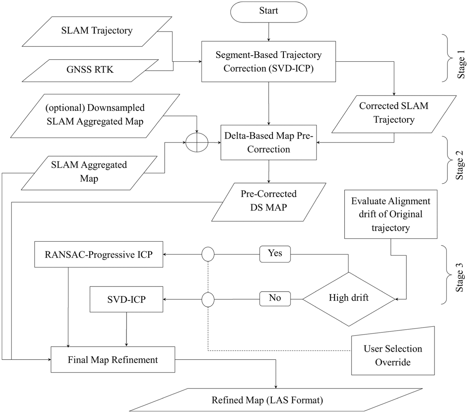
Overall pipeline architecture.
The pipeline addresses drift in three sequential modules: (1) segment-based trajectory correction using SVD-ICP; (2) delta-based map pre-correction using a hybrid time–space k-D tree; and (3) conditional map refinement via either SVD-ICP or RANSAC-progressive ICP (PICP), depending on residual drift magnitude. All major loops are parallelized to utilize multi-core central processing units (CPUs) for scalability.
For matched target P and reference Q point sets, the workflow is organized into the following stages.
Stage 1: Segment-Based Trajectory Correction (SVD Initialization + ICP Refinement)
In this stage, SLAM trajectory drift is corrected by aligning time-synchronized SLAM poses with high-accuracy GNSS RTK data. GNSS and lidar timestamps are matched by linear interpolation to form one-to-one GNSS ↔ SLAM pairs, enabling direct rigid alignment.
Each drift segment undergoes two successive steps.
a. Initial rigid transformation (SVD).
Given matched point sets, target (P = GNSS) and reference (Q = SLAM), compute their centroids.
First, compute the centroids (
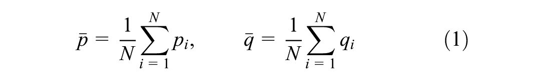
where N is the number of point correspondences in the set being aligned.
Center the points:

Form the cross-covariance matrix (H):

Compute the SVD:

where U and V are orthonormal matrices and Σ is a diagonal matrix of singular values, from the SVD of H.
Then the optimal rotation (R) and translation (t) are

b. ICP refinement (point-to-point).
The SVD result initializes ICP, which iteratively rebuilds correspondences and resolves the same least-squares problem until convergence.
Nearest-neighbor search (

The optimal transformation minimizes
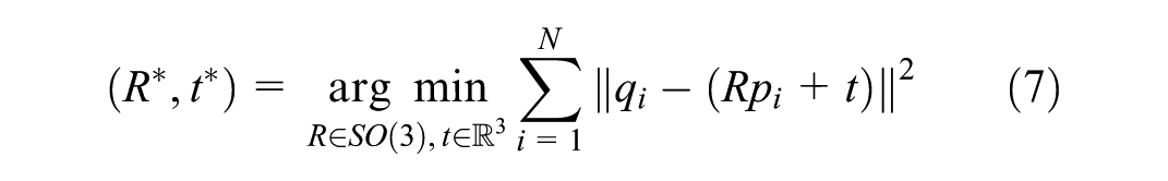
The update rule is

Iteration stops when
Each segment is processed in parallel, and the corrected pieces are concatenated into a globally aligned trajectory.
The output trajectory, including timestamps, is saved in both CSV and LAS file formats for downstream map correction.
Stage 2: Delta-Based Map Pre-Correction
Trajectory corrections from Stage 1 are propagated to the SLAM map by computing per-point deltas (ΔX, ΔY, ΔZ) between original and corrected trajectories.
Each map point is matched to its nearest trajectory delta using a hybrid 4D k-D tree that jointly considers temporal and spatial proximity.
A user-defined weighting controls the balance between time and space:

where w t and w s are normalized weights, and the time component is scaled to the spatial range so that both have comparable influence.
If w
t
= 1 (time-only), matching is purely temporal; if w
s
> 0, a combined 4D search over [scaled time, X, Y, Z] is performed. Empirically, purely temporal matching
The matched deltas shift each map point accordingly, producing a delta-corrected downsampled reference map. This intermediate output (exported in LAS file format) serves as the coarse globally referenced input for Stage 3. Because segment-wise corrections might introduce local shear, Stage 3 is utilized for final global rigid alignment.
Stage 3: Conditional Map Refinement
In the final stage, the full-resolution SLAM map is aligned to the delta-corrected reference.
The method is selected automatically from the drift ratio (default 5%) or manually by the user.
Method 3A: global rigid refinement via SVD-ICP.
Recommended for low-drift datasets, this method aligns the original aggregated map (source) with the delta-corrected reference (target).
Closed-form SVD is first used to compute the coarse rigid transformation using the same equations (Equations 1–5), followed by ICP refinement (Equations 6–8). The final transformation is applied chunk-wise to the full-resolution map.
Method 3B: robust refinement via RANSAC-PICP.
For high-drift or noisy data, RANSAC initializes a coarse transform using minimal four-point samples, each solved by SVD (Equation 5) within a robust sampling loop.
Inlier points (I k ) are defined by

Keep the transformation with the largest inlier set.
The hypothesis with the largest inlier set is retained.
The coarse model is refined through PICP, which applies successively smaller correspondence thresholds (20 → 5 → 2.5 → 1 → 0.5 → 0.2 m) and uses the previous stage’s transform as initialization, with early stopping when the root mean square error (RMSE) < 10−5.
Mean and maximum registration errors on downsampled clouds are reported, to verify convergence before the final transformation is applied to the complete point cloud.
The pipeline automatically selects between SVD-ICP (efficiency) and RANSAC-PICP (robustness) and outputs a globally corrected LAS file suitable for visualization and graphic information system (GIS) integration.
Point-to-point ICP is preferred over point-to-plane ICP, owing to the absence of reliable surface normals in the delta-propagated reference.
Altogether, the framework is modular, scalable, and robust, enabling sub-meter global accuracy from lidar SLAM datasets collected without tightly integrated IMU or GNSS inputs.
Experimental Setup and Configuration
To evaluate the performance of the proposed multi-stage correction pipeline, a series of experiments was conducted using a dataset collected with a Hesai Pandar XT32 lidar sensor, an ARDU simple AS-RTK2B-PRO GNSS receiver, and a multiband GNSS antenna. The initial SLAM trajectory and aggregated point cloud map were generated using the open-source SLAM tool LidarView 5.0.1 ( 31 ). While the GNSS data were captured in WGS84 geographic coordinates, the SLAM output was in a local frame; therefore, GNSS data were converted to Universal Transverse Mercator (UTM) Zone 12N for consistent spatial alignment. It is important to note that the SLAM process used in this study did not incorporate IMU data. The lidar-based trajectory was estimated solely from geometric constraints without inertial assistance, making the correction pipeline particularly critical for addressing drift in high-drift IMU-less SLAM scenarios.
The GNSS antenna was mounted –40 cm offset along the x-axis (in the direction of motion) and –10 cm along the z-axis relative to the lidar sensor (Figure 2b). This spatial offset was accounted for in both the global transformation and the trajectory correction processes. Since the lidar-GNSS correction framework operates purely on geometric point cloud data, radiometric phenomena, such as thermal cross-over, are not applicable to this study.
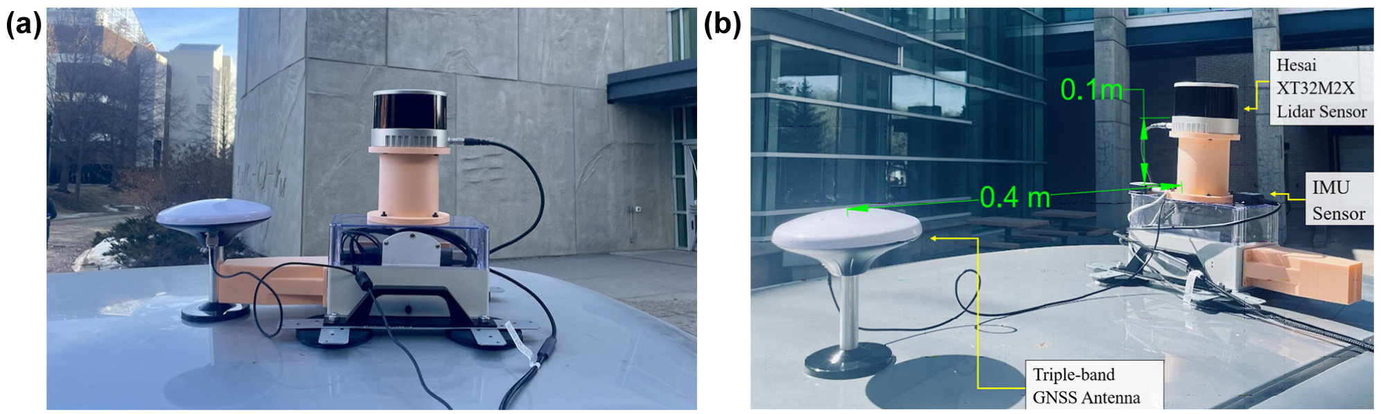
(a) Custom hardware assembly and (b) experimental layout showing the relative positioning between the lidar sensor and the GNSS antenna.
The GNSS system was operated in RTK mode using corrections received over the internet via the Networked Transport of the Radio Technical Commission for Maritime Services (RTCM) via Internet Protocol (NTRIP), which enables real-time delivery of GNSS correction data from a base station (or caster) to a mobile rover, substantially enhancing positional accuracy. In this study, correction streams were accessed from publicly available or regional Canadian NTRIP casters ( 32 ). This setup enabled high-precision positioning, achieving approximately 1 cm accuracy in 2D and 2 cm in 3D across all seven control points. A snapshot of this accuracy, as visualized in u-center software, is shown in Figure 3b. This was essential to ensure that the control points used for evaluation represent high-confidence ground truth references.
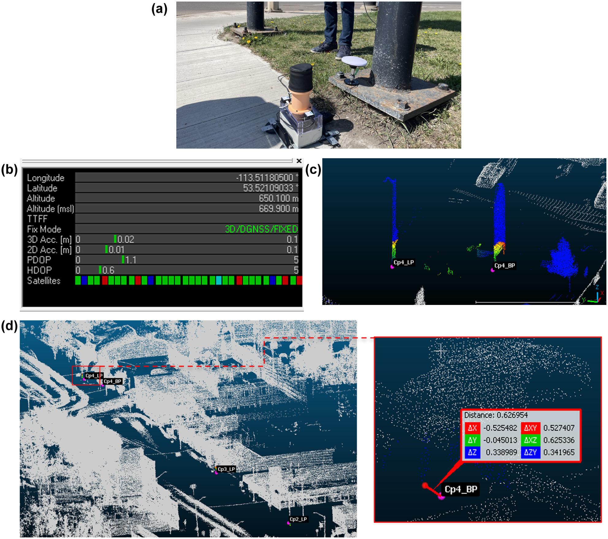
(a) Field data measurement, (b) GNSS accuracy and fix status, (c) sample of extracted light pole and advertisement board from the point cloud, and (d) distance measurement against the control point.
Pipeline Configuration
The multi-stage correction pipeline was configured using the parameter values summarized in Table 1. These parameters were tuned iteratively across several trials to balance processing speed and alignment accuracy, as higher settings yielded only marginal accuracy gains at the cost of runtime. The RANSAC configuration applied strict inlier thresholds to enhance robustness against outliers, while the ICP stage was fine-tuned with a small root mean square (RMS) convergence threshold and iterative refinement. A progressive ICP scheme was used, gradually tightening the correspondence threshold across six stages: [20.0, 5.0, 2.5, 1.0, 0.5, 0.2]. This allowed the algorithm to converge on coarse alignments first and then refine the transformation with increasing precision.
Pipeline Parameter Settings
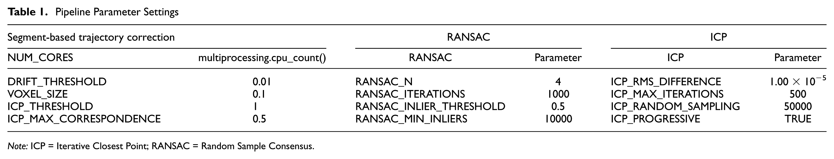
Note: ICP = Iterative Closest Point; RANSAC = Random Sample Consensus.
Evaluation Metrics
The pipeline performance was assessed using the following metrics.
■ Trajectory accuracy (Stage 1). RMSE between corrected trajectory and GNSS RTK.
■ Map accuracy (Stage 3). Average representative cloud to GNSS point coordinate RMSE; per-point accuracy, measured against seven GNSS RTK control points.
■ Qualitative analysis. Visual comparisons of point cloud maps overlaid on satellite basemaps, used to assess alignment improvements and consistency.
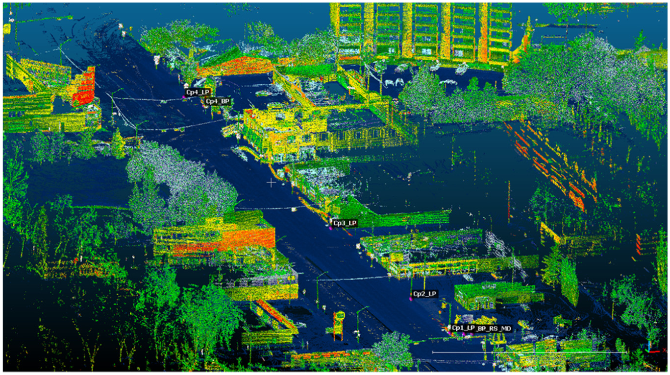
Representative evaluation locations were selected at the bases of light poles or advertisement boards, as these features are easily identifiable in the point cloud map (Figure 3c). The cloth simulation filter (CSF) presented by Zhang et al. (33) was applied to separate ground and non-ground points, facilitating the accurate selection of representative reference points.
Results
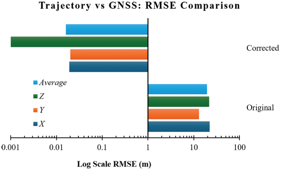
The results in Table 2 and Figures 4 and 5 show a substantial reduction in RMSE across all axes after Stage 1 trajectory correction. The RMSE against the GNSS RTK reference was significantly reduced, from 19.4 m to 0.016 m on average, indicating successful mitigation of the primary trajectory drift. The average computation time for this stage was approximately 1.9 s. The sub-centimeter corrected RMSE in all directions highlights the pipeline’s robustness in mitigating SLAM drift. Figure 5 shows both 2D and 3D representations of the GNSS RTK reference path alongside the original and corrected SLAM trajectories, illustrating the alignment improvements achieved through the correction pipeline.
Stage 1 Trajectory Correction Performance
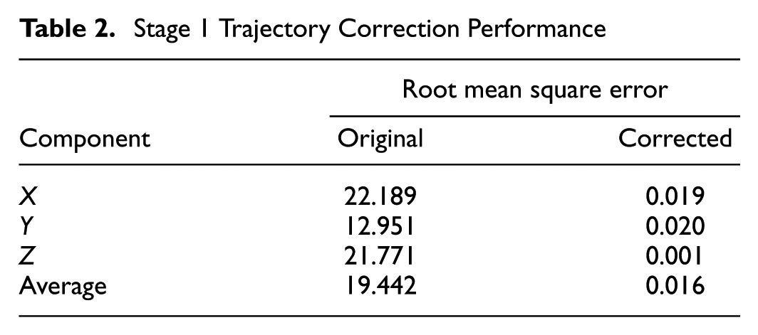
Stage 1 trajectory correction performance.
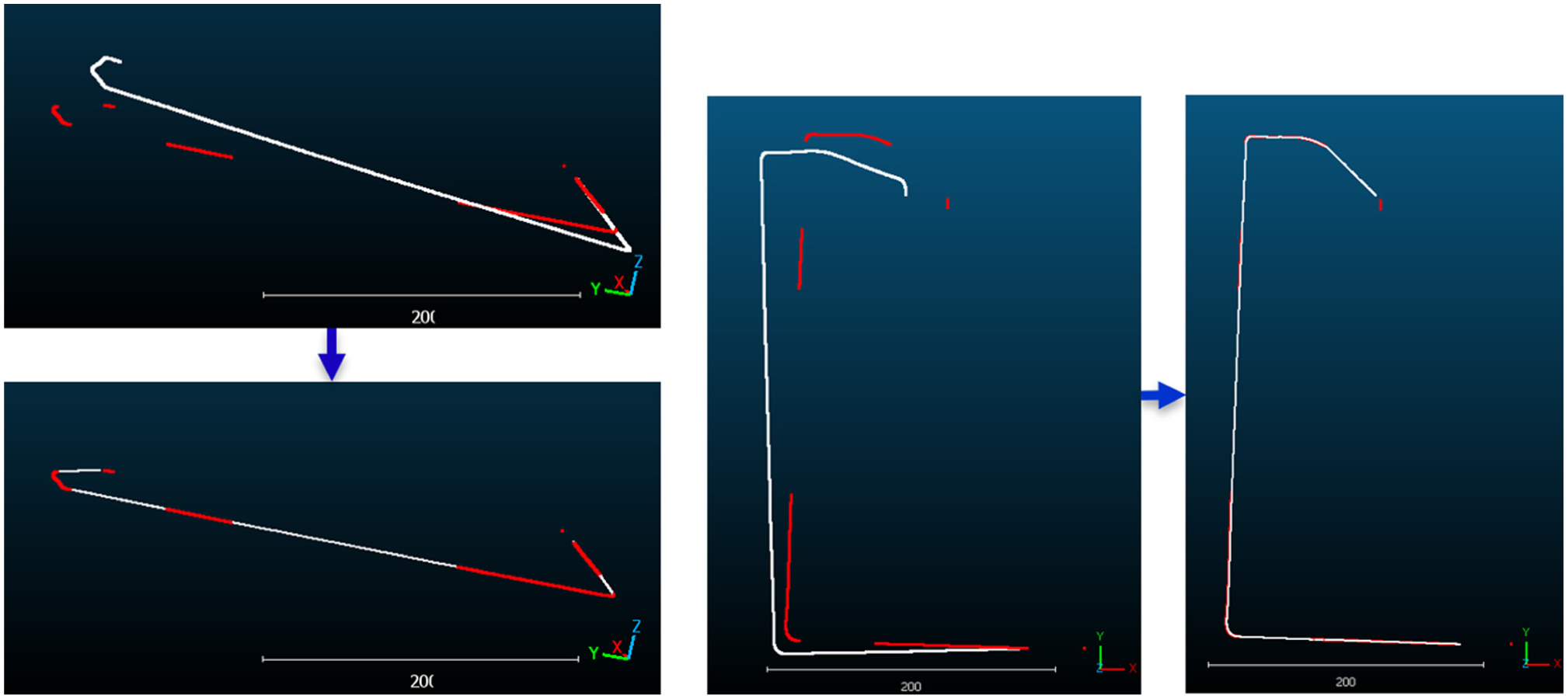
Visual representation of trajectory correction: GNSS trajectory (red); Lidar trajectory (white).
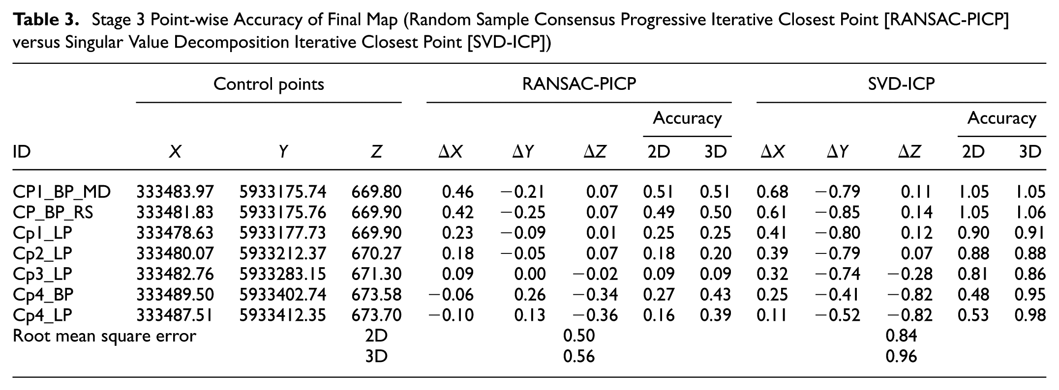
As shown in Table 3, the distances between the GNSS RTK control points and the corresponding representative point cloud locations highlight the relative performance of the refinement methods. Across all seven control points, the RANSAC-PICP method consistently outperformed SVD-ICP, demonstrating lower 2D and 3D RMSEs and indicating superior global alignment and reduced residual misalignment.
Stage 3 Point-wise Accuracy of Final Map (Random Sample Consensus Progressive Iterative Closest Point [RANSAC-PICP] versus Singular Value Decomposition Iterative Closest Point [SVD-ICP])
As shown in Figure 6, the RANSAC-PICP method achieved smaller RMSEs than the SVD-ICP method and produced a tighter spatial fit with the GNSS reference. The close-up around Control Point 2 (CP2) shows sub-decimeter agreement between the corrected lidar map and the surveyed ground position.
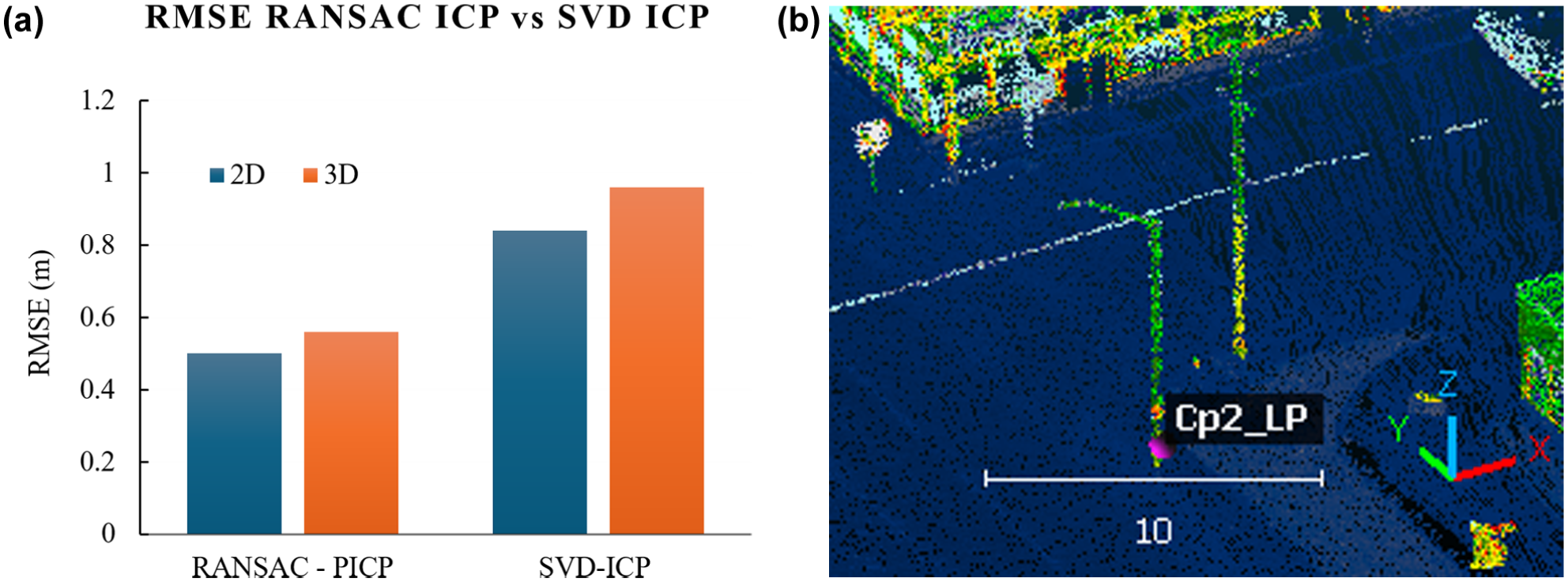
(a) Comparison of root mean square error (RMSE) between correction methods based on Random Sample Consensus progressive Iterative Closest Point (RANSAC-PICP) and Singular Value Decomposition Iterative Closest Point (SVD-ICP) and (b) close-up view of corrected (RANSAC-PICP) lidar map against Control Point 2 (CP2).
The visual comparisons in Figures 7 to 12 further demonstrate the effectiveness of the proposed correction pipeline across different scans and refinement strategies. In Figure 7 (Scan 1), both the corrected trajectory and the transformed point cloud exhibit clear improvements in global alignment. The corrected trajectory (black) closely follows the GNSS reference (red), and the point cloud map aligns well with visible road features. The 3D view in Figure 8 further confirms the spatial consistency of the corrected point cloud with GNSS RTK control points, indicating high local accuracy.
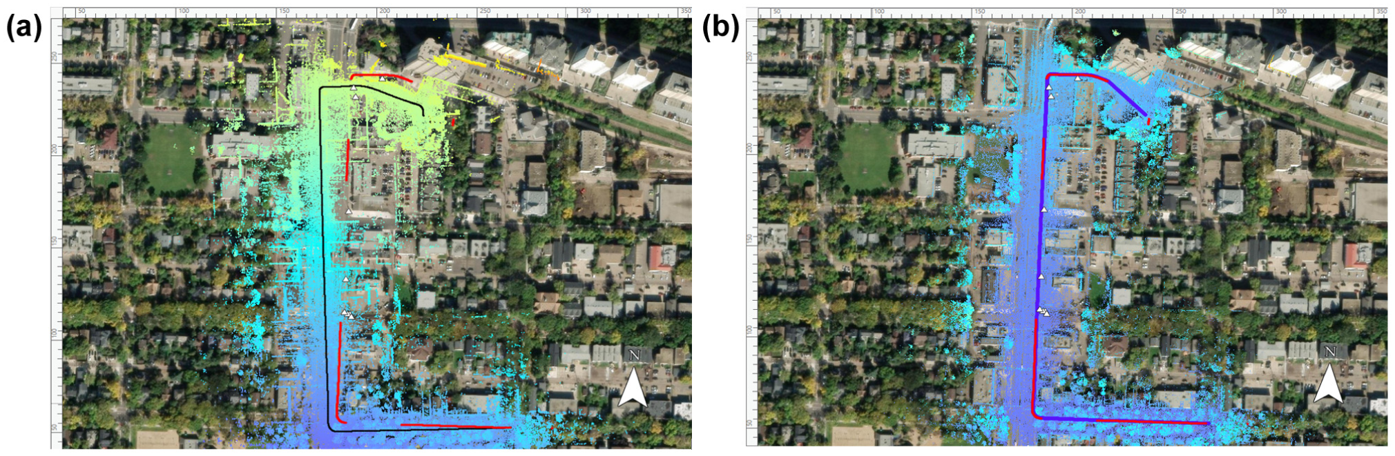
Scan 1. Overlay of point clouds on satellite basemap: (a) GNSS trajectory (red), globally transformed simultaneous localization and mapping (SLAM) trajectory (black), and corresponding transformed map; (b) GNSS trajectory (red), corrected trajectory (black), and final corrected map.
Scan 1. 3D visualization of corrected point cloud map with overlaid GNSS real-time kinematic (RTK) control points.
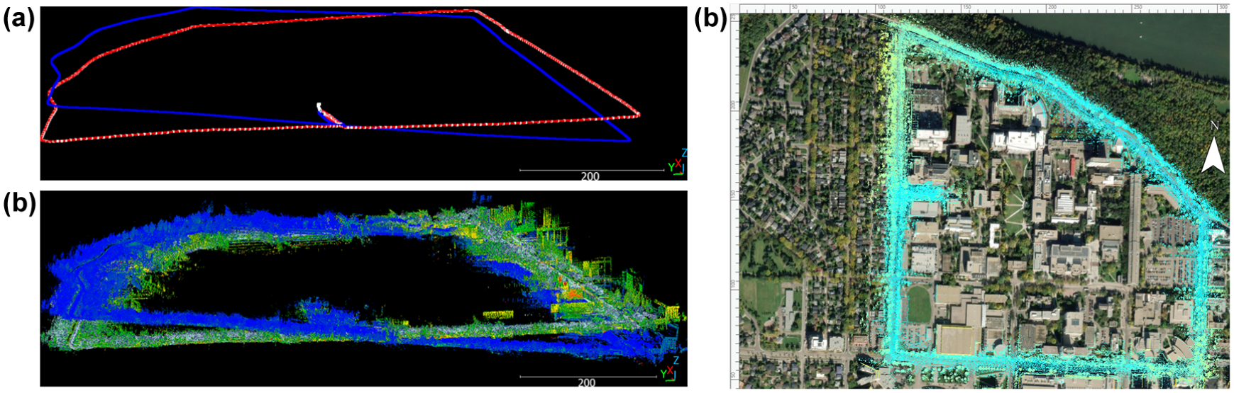
Scan 2. (a) GNSS trajectory (red), globally transformed simultaneous localization and mapping (SLAM) trajectory (blue), and corrected trajectory (white); (b) comparison between globally transformed point cloud map (blue) and corrected cloud map (green); (c) overlay of point clouds on satellite basemap, showing corrected and transformed map.
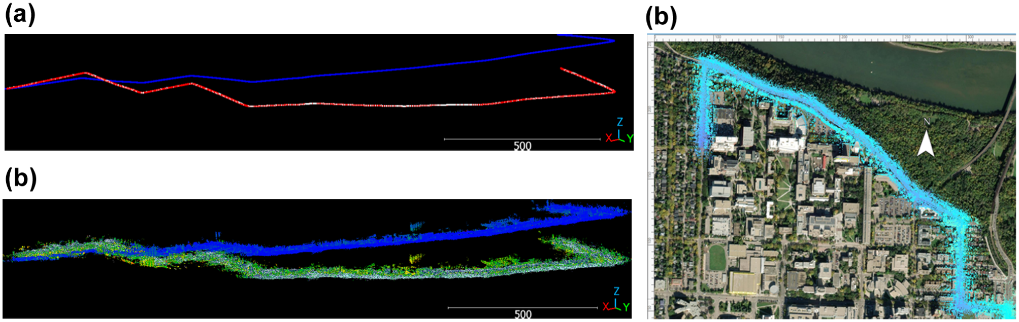
Scan 3: (a) GNSS trajectory (red), globally transformed simultaneous localization and mapping (SLAM) trajectory (blue), and corrected trajectory (white); (b) comparison between globally transformed point cloud map (blue) and corrected point cloud map (green); (c) overlay of point clouds on satellite basemap, showing corrected and transformed map.
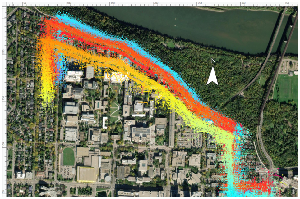
Overlay of globally transformed (yellow), singular value decomposition Iterative Closest Point (SVD-ICP)-corrected (orange), and Random Sample Consensus progressive Iterative Closest Point (RANSAC-PICP)-corrected (cyan) point clouds on satellite basemap.
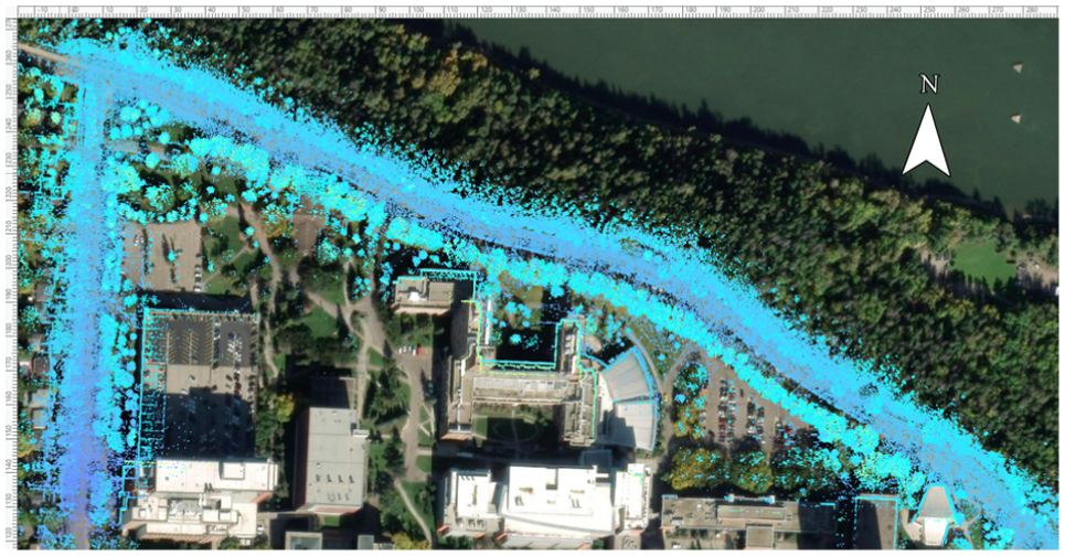
Close-up view of Random Sample Consensus progressive Iterative Closest Point (RANSAC-PICP)-corrected point cloud (cyan), overlaid on satellite basemap.
In Scans 2 and 3 (Figures 9 and 10), similar improvements are evident. The corrected trajectories (white) in Figures 9a and 10a more accurately follow the GNSS trajectories, compared with the globally transformed SLAM trajectory (blue). The point cloud comparisons in Figures 9b and 10b show that a significant transformation, particularly in 3D rotation, was applied during correction. This is visually reinforced in Figures 9c and 10c, where the corrected point clouds overlay the satellite basemap well, providing a clear validation of the drift correction.
Figure 11 presents a side-by-side comparison of the globally transformed (yellow), SVD-ICP-corrected (orange), and RANSAC-PICP-corrected (cyan) point clouds. The RANSAC-PICP result exhibits the closest alignment with real-world features, while the SVD-ICP corrected map shows visible residual misalignments—especially in regions affected by local deformation. The close-up in Figure 12 highlights how the RANSAC-PICP-corrected map closely matches the satellite basemap features, including the edges of rectangular and curved buildings, offering strong visual confirmation of its improved geometric accuracy.
Discussion
The results demonstrate that the proposed modular pipeline effectively enhances both the global accuracy and internal consistency of lidar SLAM maps through GNSS-aided post-processing. Each stage comprises a distinct role, including trajectory correction, map propagation, and final geometric refinement, progressively reducing accumulated drift. The results achieve centimeter-level accuracy, affirming the reliability of segment-wise trajectory alignment using RTK data.
Method 3A (SVD-ICP) offers a computationally lightweight solution when the residual misalignment after delta correction is small and largely rigid. This method is well-suited for structured and well-behaved datasets, where the SLAM trajectory does not exhibit significant local deformation. However, SLAM systems can introduce inconsistencies—through motion-induced distortion, sparse features, or lack of loop closures—that result in non-uniform drift or localized shear. Similarly, the delta-based correction in Stage 2, while efficient, assumes rigid local motion based on trajectory deltas. This assumption might not hold in complex urban environments, potentially leading to discontinuities in the intermediate reference map.
This is where Method 3B (RANSAC-PICP) proves its value. The RANSAC component robustly estimates an initial transformation by selecting consensus-based correspondences and rejecting outliers, even in the presence of local inconsistencies or severe drift. Each hypothesis is computed from four-point samples (n = 4) solved via the same SVD formulation used in Method 3A and processed in parallel batches across CPU cores. The resulting estimate is further refined through multi-stage PICP, which successively tightens correspondence thresholds (20 → 5 → 2.5 → 1 → 0.5 → 0.1 m), with early stopping when the inlier RMSE < 10−5, achieving stable convergence. While computationally more intensive than SVD-ICP, the RANSAC-PICP process proved essential in scenarios with significant residual misalignment.
The performance difference becomes particularly pronounced under conditions of long-range SLAM trajectories without loop closure, where cumulative drift manifests as large-scale map distortion. For example, in one open-SLAM experiment (scan 3) with a 7.26% drift ratio—amounting to nearly 192 m over a 2.6 km trajectory—RANSAC-PICP produced visually superior results (Figure 11). The corrected map, when rendered in ArcGIS Pro, aligned closely with satellite basemaps, while the SVD-ICP version exhibited noticeable offsets. This underscores the importance of robust registration methods in post-processing, particularly in open-ended or infrastructure-scale mapping, where absolute consistency is critical.
The final alignment accuracy further supports this conclusion. As shown in Table 3, RANSAC-PICP achieved smaller RMSEs at GNSS RTK control points, with a 2D RMSE of 0.50 m and a 3D RMSE of 0.56 m, compared with 0.84 m (2D) and 0.96 m (3D) for SVD-ICP refinement. This accuracy difference—though moderate numerically—translates to visible improvements in map alignment and consistency, particularly in applications requiring centimeter- to decimeter-level precision, and becomes increasingly significant in longer SLAM trajectories, where small residual errors can accumulate into large-scale positional deviations.
The pipeline’s design also reflects a meaningful trade-off between accuracy and efficiency. The SVD-ICP method was completed in approximately 29.7 s, while the RANSAC-PICP workflow took 71.9 s to process over 12 million points. This performance supports adaptive correction workflows, where drift metrics (such as the observed drift ratio) can guide method selection to balance runtime with expected alignment quality.
A critical methodological finding is related to the ICP variant employed in Stage 3. While point-to-plane ICP is often favored in structured environments for its faster convergence, experiments revealed it to be unstable when applied to the Stage 2 reference map. The intermediate map, constructed through delta propagation rather than direct SLAM optimization, might lack reliable planar structure for accurate normal estimation. As such, point-to-point ICP was adopted, offering superior stability without requiring surface normals. Despite its slower convergence, this choice ensured reliable alignment in diverse conditions, particularly when local surface structure was sparse or degraded. The pipeline’s strength lies in this adaptability, combined with systematic drift handling, efficient delta-based propagation, parallelized RANSAC computation, and compatibility with standard formats, such as LAS.
An important architectural insight is that, although the ICP refinement enables computation of a single rigid transformation, this is computed relative to a non-rigidly corrected reference map. As a result, the rigid alignment indirectly incorporates the effects of local deformation, offering a compromise between rigid model simplicity and non-rigid responsiveness. However, because only a single global transformation is ultimately applied to the point cloud, true non-rigid inconsistencies remain uncorrected and are only absorbed where they align with the estimated rigid fit. This motivates future research into integrating non-rigid refinement modules to address these structural deviations explicitly.
In addition, the pipeline’s accuracy depends primarily on the availability of reliable GNSS control points, rather than continuous high-frequency GNSS coverage. Unlike real-time frameworks, which require temporally dense GNSS and IMU data for tightly coupled optimization, the proposed approach functions effectively with sparse but accurate GNSS references. This makes it particularly suitable for post-SLAM correction in environments where GNSS signals are intermittent or partially obstructed. The method remains robust as long as well-distributed control points are available to anchor the trajectory segments. Future work will be focused on extending this framework toward semi-online operation and incorporating non-rigid refinement to further improve local consistency without requiring dense GNSS sampling.
Beyond accuracy, an important advantage of the proposed framework lies in its scalability and modular design. The pipeline efficiently processed over 12 million lidar points in less than 90 s using a standard workstation (Dell Precision 3680, Intel Core i9-14900K CPU @ 3.2 GHz, 32 cores, 64 GB random access memory, Windows 11 64-bit). This demonstrates the computational efficiency of the method, even without graphics processing unit (GPU) acceleration. Each stage—trajectory correction, delta propagation, and final refinement—is independent, allowing flexible adaptation to various SLAM outputs and sensor configurations. The use of standard LAS 1.4 output files ensures compatibility with GIS and photogrammetric workflows, extending the framework’s applicability to large-scale roadway mapping, autonomous-vehicle dataset generation, and digital-twin modeling tasks.
Conclusions
This paper introduces a multi-stage post-processing pipeline aimed at enhancing the global consistency and spatial accuracy of lidar SLAM-derived maps through the integration of high-precision GNSS RTK data. The pipeline consists of three sequential stages: (1) segment-based trajectory correction via SVD-ICP; (2) delta-based propagation of corrections to the point cloud through a hybrid time–space k-D tree; and (3) a conditional final refinement step employing either SVD-ICP or RANSAC-PICP, selected according to residual drift magnitude.
Experimental results show substantial reductions in both trajectory and map errors, achieving sub-meter RMSE, even under high-drift conditions where SLAM was conducted without IMU integration. The pipeline’s flexibility, which allows for a choice between fast and robust refinement strategies based on drift severity, makes it suitable for a broad spectrum of mapping applications, including urban infrastructure surveys, autonomous-vehicle dataset generation, and offline map refinement.
Processing of over 12 million points in less than 90 s confirms the framework’s scalability. Through its modular structure, computational efficiency, and compatibility with standard geospatial formats, the proposed approach provides a practical and reproducible solution for post-processing SLAM datasets. Its ability to correct accumulated drift and improve spatial alignment underscores its potential for integration in larger geospatial workflows and real-time GNSS-SLAM mapping systems.
Footnotes
Acknowledgements
The author used artificial intelligence (AI) language models, including ChatGPT (GPT-4.0), to assist with code debugging and grammar refinement during manuscript preparation.
Author Contributions
The authors confirm contribution to the paper as follows: study conception and design: F. N. Birhane, K. El-Basyouny; data collection: F. N. Birhane, A. M. Sakr, K. Shah; analysis and interpretation of results: F. N. Birhane; draft manuscript preparation: F. N. Birhane. All authors reviewed the results and approved the final version of the manuscript.
Declaration of Conflicting Interests
The authors declared the following potential conflicts of interest with respect to the research, authorship, and/or publication of this article: Karim El-Basyouny is a member of Transportation Research Record’s Editorial Board. All other authors declared no potential conflicts of interest with respect to the research, authorship, and/or publication of this article.
Funding
The authors disclosed receipt of the following financial support for the research, authorship, and/or publication of this article: funding from the Natural Sciences and Engineering Research Council of Canada (NSERC) (grant no. ALLRP 586279-23).
Data Accessibility Statement
The algorithms and scripts used in this study are openly available at: ![]() .The repository provides a reference implementation of the complete modular GNSS-aided post-SLAM correction pipeline, including GNSS pre-processing tools, global coordinate transformation scripts, and post-SLAM correction modules, along with documentation to support transparency and reproducibility.
.The repository provides a reference implementation of the complete modular GNSS-aided post-SLAM correction pipeline, including GNSS pre-processing tools, global coordinate transformation scripts, and post-SLAM correction modules, along with documentation to support transparency and reproducibility.