
Abstract
Estimating behavioral parameters for mode choice typically relies on revealed- or stated preference data. However, applying GPS-based revealed preference (GPS-RP) panel data in modeling mode choice, particularly in response to shocks or policy interventions, remains relatively rare and methodologically under-explored. This paper discusses the preparation, processing, filtering, and modeling of (semi-)automated travel diaries collected over 3 months, including the 9-Euro-Ticket fare policy intervention in Germany in 2022. By estimating two multinomial logit models, we investigated how this intervention influenced the value of travel time savings (VTTS) across different modes. Our findings revealed a substantial reduction in VTTS for public transportation during the intervention period, with values approximately half those in the months following the intervention, highlighting the profound impact of this nearly fare-free policy. This study debates the difficulties and complexities of estimating VTTS using GPS-RP data for urban travel behavior. It underscores the importance of robust preprocessing and filtering methodologies when handling complex GPS data, and discusses how the intervention’s effects on VTTS and project appraisal could inform future transportation policy and investment strategies.
Introduction
The analysis and modeling of transportation mode choice is one of the most extensively studied and frequently addressed topics within the transportation field ( 1 , 2 ). Application of the resulting models includes not only purely engineering uses ( 3 , 4 ) but also project appraisal and policy analysis ( 5 , 6 ). They provide key quantitative indicators, such as marginal rate of substitutions, willingness to pay, and elasticities, which guide investments and pricing policies ( 7 ). A popular family of discrete choice models, the random utility model (RUM), is based on the assumption of utility-maximizing behavior by the decision maker and captures the probabilistic nature of individual choices ( 1 ). Researchers use this theoretical foundation to derive robust insights into travel behavior and its responsiveness to various interventions ( 8 ).
In transportation modeling practice, data can generally be classified into revealed preference (RP) data, which describes the actual observed or reported travel behavior of individuals, and stated preference (SP) data, which illustrates individuals’ preferences in hypothetical choice scenarios set by the researcher ( 1 ). Studies also often utilize pooled RP/SP data, leveraging the strengths of both types ( 9 – 11 ). Until the 1980s, mode choice modeling primarily relied on RP data collected through traditional pen-and-paper travel diaries, which had been in use since the 1950s ( 12 , 13 ). These data were considered reliable for capturing participants’ preferences and the context of their choices, and were widely available. However, travel diaries typically record travel information for only a single day or week, limiting the number of observations per participant and requiring large samples to ensure representative and robust results. Additional drawbacks include high collinearity and low variability among attributes ( 14 ), as well as frequent misreporting and underreporting of trips ( 2 , 15 ). To address these limitations, researchers increasingly turned to stated-choice (SC) experiments, which present participants with hypothetical but realistic choice scenarios in a controlled setting. SC methods offer greater control over the experimental design, enable the inclusion of nonexisting alternatives such as new transport modes, and allow the collection of multiple observations per participant within a short timeframe. However, they are susceptible to various response biases (lexicographic behavior, strategic behavior, lack of consequentiality bias, etc.), some of which are difficult to control and mitigate ( 12 , 16 , 17 ). Despite these concerns, numerous studies have validated SC-derived economic indicators through comparisons with those obtained using RP data ( 12 ), showing that SC experiments can effectively reveal trade-offs between attributes, even if they may not fully capture real-world behavior. Nevertheless, RP data remain relevant and are still used—both alone ( 18 ) and combined with SP data—to enhance the realism of choice scenarios ( 10 ) or improve model robustness via joint estimation ( 19 , 20 ).
The emergence of new technologies, particularly the popularization of GPS and connected personal devices, has opened up new possibilities in travel data collection ( 21 – 24 ). Over the past two decades, the processing of GPS data to infer trips, travel modes, and trip purposes has gained tremendous academic and practical interest, leading to substantial methodological advancements ( 25 – 28 ). These developments, coupled with the advent of dedicated smartphone applications, now enable the collection of large volumes of high-accuracy data with minimal user effort, facilitating the creation of (semi-)automated travel diaries ( 17 , 29 , 30 ). This type of GPS-based RP data (GPS-RP) are increasingly appealing owing to their relatively low data-collection cost per trip. Their use has already gained popularity in diverse transport-related problems, such as trip generation ( 31 , 32 ), destination choice ( 33 ), and route choice modeling ( 34 , 35 ). However, research on mode choice utilizing smartphone-based GPS tracking remains limited, with most previous investigations being either descriptive in nature ( 36 , 37 ) or employing machine learning techniques, which are well-suited to handling the extensive datasets often associated with this technology and require fewer specific parameter settings ( 38 – 40 ). Even though there is growing research using smartphone tracking for public policy appraisal ( 41 – 43 ) and disruptions like the COVID-19 crisis ( 44 – 46 ), the potential for utilizing geotemporal data for inferential analysis is far from exhausted. There remains a remarkable gap in research utilizing long-term panel GPS data in combination with household surveys. This gap not only pertains to using such data to address transportation research questions but also extends to discussing methodologies and best practices for the data processing required for accurate analysis.
There are smartphone-based RP datasets like the MOBIS dataset ( 43 ), which includes GPS tracking data from 3,680 individuals over an 8-week period, and the ETH-IVT Travel Diary, which encompasses data from 6,838 trips made by 172 users in Zurich, Switzerland, collected during 2019 and 2020 ( 47 ). However, to the best of our knowledge, no traditional discrete choice models, like the multinomial logit (MNL), for mode choice have been estimated using these data sources. Meister et al. used the MOBIS dataset to analyze how individuals’ travel times changed across different transport modes during and after the COVID-19 lockdown, compared with a prepandemic reference period ( 48 ). Their approach relied on a mixed multiple discrete-continuous extreme value (MMDCEV) model, which is only loosely related to traditional discrete choice models. Unlike MNL models, the MMDCEV does not require nonchosen alternatives, and it does not model single discrete choices per trip. Instead, it estimates continuous quantities of (travel) consumption per mode on a weekly basis. Marra and Corman route choice modeled on the ETH-IVT Travel Diary data, but using a deep learning model ( 49 ).
We are aware of only two studies that have employed long-term panel GPS data in conjunction with household survey information to estimate theory-driven mode choice models. First, Tsoleridis et al used a 2-week travel diary captured through smartphone GPS tracking to derive transport appraisal values ( 17 ). Second, Link investigated inertia effects in transportation modes before and during a German price intervention, the 9-Euro-Ticket, which is also the focus of this study ( 42 ). This intervention, introduced in spring 2022 by the German parliament to alleviate rising living costs resulting from the Ukraine war, comprised a 3-month fuel excise tax cut and the introduction of a public transportation (PT) season ticket for €9 per month (approximately $9.45 using the 2022 exchange rate of 1 EUR = 1.05 USD). This ticket was valid on all local and regional services but excluded long-distance PT. The 9-Euro-Ticket, which was sold 52 million times, represented a groundbreaking initiative in Germany since it not only introduced almost fare-free PT but also harmonized fares across approximately 60 different tariff associations. This policy intervention was implemented during the months of June, July, and August, providing a quasi-natural experiment that allowed researchers to measure changes in travelers’ behavior resulting from the ticket’s availability ( 50 ). Given the ticket’s novelty, it was extensively researched. The Association of German Transport Companies conducted a survey with 200,000 respondents across Germany, which revealed that around 20% of the ticket customers were new customers to PT and that 17% of the trips had been shifted from other transportation modes. The ticket was well received, depicted in a high approval rate of 88% of the users ( 51 ). Another smartphone tracking study indicated that the 9-Euro-Ticket did not alter daily mobility patterns but instead prompted an increase in leisure travel, particularly at the start and conclusion of the ticket’s validity period ( 52 ). These findings are in line with the general research on the effects of (almost) fare-free PT on travel behavior; such interventions, even if short-term, can reshape travel behavior by lowering monetary barriers, altering perceptions, and inducing (limited) demand. However, these effects vary with context, local habits, and policy setup and warrant additional analysis ( 53 ).
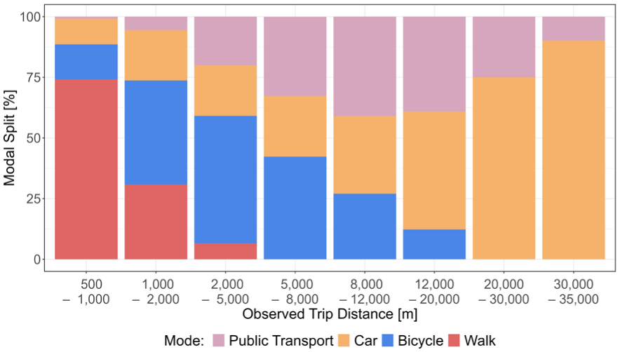
In this research, we employed a 3-month sample of GPS panel tracking data from the Mobilität.Leben project to explore the effects of the 9-Euro-Ticket on the value of travel time savings (VTTS). Firstly, we make a methodological contribution by addressing a missing link in the existing literature, detailing the processing steps necessary to transform raw GPS data into a format suitable for discrete choice modeling. This includes the generation of mode alternatives for observed trips and an extensive filtering process to ensure the final dataset adheres to the behavioral assumptions of RUMs. Although our primary focus is on data processing, we also estimate two MNL models and discuss the possible approaches to account for a price intervention using panel GPS data. Secondly, this research contributes to transport policy assessment by comparing VTTS during and after the price intervention. There is a notable lack of studies examining how pricing measures, such as road tolls, ticket subsidies, or fare-free PT, affect VTTS based on GPS data. Carrion and Levinson use RP data from GPS-tracked trips to estimate the value of travel time and reliability for commuters choosing between tolled and toll-free routes ( 54 ). However, they do not investigate how VTTS changes before and after the introduction of the toll, leaving open the question of how pricing interventions influence these trade-offs. Since behavioral VTTS captures the real-world exchange between time and money, it is highly relevant for evaluating the effectiveness of such interventions. We hypothesized that when money becomes less scarce relative to time, as in the case of the 9-Euro-Ticket, this alters the observed sensitivity to travel time in discrete choice models ( 55 ). In the following analysis, we test this hypothesis and explore how the price intervention affects VTTS, thereby contributing to the broader discussion on travelers’ sensitivity to time versus cost under different pricing regimes. Importantly, the analysis focuses on short urban trips—as depicted in Figure 1—addressing for the first time how the 9-Euro-Ticket influencs VTTS. The remainder of this paper is organized as follows: first, we describe the data and the processing steps. Second, we detail the generation of the choice sets and the data filtering methods used. This leads to a descriptive analysis of the final dataset. We then outline our modeling approach, which sets the stage for presenting our findings. Finally, we conclude with a discussion of the results and offer insights for future research directions.
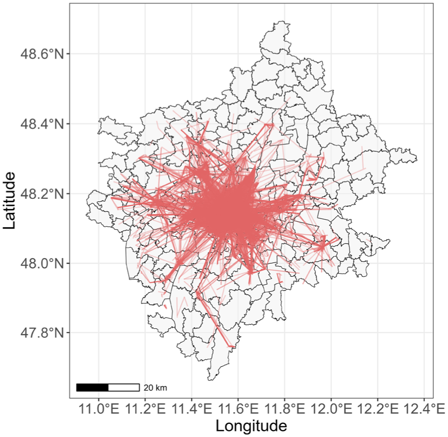
Origin–destination trips of the final dataset mapped on Munich.
Techniques for Utilizing GPS Data
With the roll-out of the 9-Euro-Ticket in June 2022, the Mobilität.Leben research project was initiated to assess this unprecedented almost free PT policy, and it was later extended into 2023 following the announcement of the successor ticket, the 49-Euro Deutschlandticket. Overall, the data collection spanned 20 months ( 50 ) and included a multiwave survey with 2,624 participants ( 56 ). This research initiative faced a brief planning window between the announcement of the 9-Euro-Ticket and its introduction in June 2022. The ad hoc nature of the initial phase of Mobilität.Leben led to a dual recruitment approach. A panel agency conducted a nationwide survey distribution, while a targeted media campaign in the Munich metropolitan area recruited participants for the GPS tracking component. Owing to technical and logistical constraints, only participants recruited via the regional media campaign (n = 1,140) used the GPS-based tracking app, resulting in the GPS data being concentrated primarily in Munich. The survey collected sociodemographic data, mobility tool ownership, attitudinal information, and travel behavior insights. The app, developed by the software company Motiontag, recorded participants’ movements and stays (i.e., a stationary activity with a specific purpose). It also allowed users to edit tracks (i.e., representing a single-mode movement) and stays (e.g., for correcting erroneous entries, modifying the automatically detected transportation mode, and merging consecutive tracks) and select the stay’s purpose, thus creating a semipassive travel diary. A typical tour in the app is illustrated in Figure 2. Since the experiment had to be set up at short notice, the recruitment of the participants through the media campaign limited the sample’s representativeness. In this paper, we utilized a subset of the Mobilität.Leben data, specifically from the second month (July) of the 9-Euro-Ticket (intervention), and compared it with data from September and October, when the 9-Euro-Ticket was no longer in effect (postintervention). August was excluded because it was a public holiday period. The dataset encompassed 3 months, including 154,605 trips by 785 users, before the processing procedures detailed below.
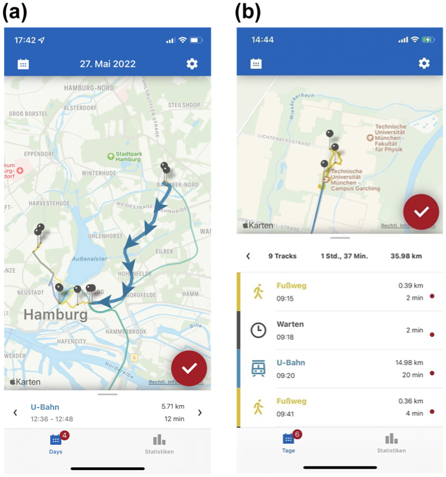
User interface of the Motiontag app: (a) tour-based map visualization and (b) track validation interface.
Choice Set Generation
The GPS tracking data, as provided by Motiontag, were in the first step validated, enriched, and transformed into a (semi-)passive travel survey. This extensive preprocessing stage is described in detail in a technical paper by Dahmen et al. (57) and, although it falls out of the scope of this publication, we begin this section by providing a brief introduction to it. Building on their work, we included further filtering and data enrichment steps to make the RP data suitable for mode choice modeling. We first detail the identification of nonchosen mode alternative characteristics and explain the calculation of costs for both nonchosen and chosen alternatives. Subsequently, the integration of weather data is discussed. Finally, the removal of outliers is examined.
Generation of Travel Diaries from GPS Smartphone-Based Data
Raw data from passive tracking devices or apps typically consist of a series of coordinates paired with timestamps, recorded at (ir-)regular intervals. However, these data lack contextual information: they do not reveal whether each recorded point belongs to a stationary activity (nor its purpose) or to a movement (and the mode of transportation used). In the first step, the recorded intervals are segmented into stays and moves through rule-based or data-driven methods. In the second step, the movement segments are enriched by automatically identifying the transportation mode based on speed, acceleration, transportation network proximity, distance between points, and so forth ( 58 – 60 ). The stays must be labeled with their corresponding purposes by the user. Once labeled, the system is designed to automatically detect and assign the same purpose if the user visits that specific location again. Motiontag’s proprietary technology performs these steps by streamlining the process and creates automated (draft) travel diaries that, after in-app user correction or validation, become (semi-)automated travel diaries.
Although (semi-)automated travel diaries offer valuable mobility insights, errors in GPS tracking and limited user engagement with the draft version can introduce defective and missing entries that have an impact on mobility behavior analysis and modeling. As already mentioned, Motiontag’s diaries provide only two types of elements: tracks (representing a single-mode movement) and stays (a stationary activity with a specific purpose). However, the study of travel behavior is mostly based on trips, which comprise one or multiple tracks and waiting or stationary stays between consecutive tracks (e.g. people waiting for a connecting service). The decision to travel by a specific mode is based on the overall origin and destination of a trip, rather than on individual segments. To address these limitations, Dahmen et al. developed a quality enhancement method for large-scale, long-duration (semi-)passive travel diaries ( 57 ). Their approach included numerous sanity checks and eliminated errors (e.g., unrealistic speeds, abnormally short moves or stays) or corrected them by merging consecutive tracks with the same mode and reconnecting fragmented stays. The thresholds used by Dahmen et al. were either derived from the analysis of the Mobilität.Leben dataset (e.g., the X% fastest speed of a mode) or adapted from other studies ( 57 ). The enhancement method also detects trips and enriches the dataset by map-matching movements to the road/street network.
Although these quality enhancement methods established critical quality standards and serve as a foundation for subsequent data enrichment processes, the cleaning and filtering undertaken in Dahmen et al.’s study were not conceived to create a dataset suitable for discrete choice modeling but rather to derive mobility analyses ( 57 ). For this reason, further filtering and processing are needed, although some of the steps and thresholds overlap between both works (i.e., this study applies stricter thresholds).
Data Enhancement Process
Travel Time and Travel Distance
We limited our analysis to four main transportation modes: walking, cycling, car, and PT. We included only trips within Munich’s transit authority—Münchner Verkehrs- und Tarifverbund (MVV)—zone because it operates as a single tariff system with harmonized zones and ticket options, allowing for consistent cost calculations and regional comparability of PT trips. To make the observed trips suitable for modeling, it was essential to enrich them with information about nonchosen alternatives and their attributes ( 17 , 42 ). This involved estimating travel times, costs, access/egress, and waiting times for both chosen and nonchosen modes ( 61 ). To use the trip-based information efficiently for estimating mode choice models, we followed the main-mode approach ( 62 ). This considers the mode used for the longest portion of the trip to be the primary mode, allowing the comparison of specific modes with potential alternatives. To make the generated alternatives comparable, filtering was necessary. Generating all potential multimodal alternatives in urban settings like Munich, known for its complex travel demand patterns and numerous travel options, would be highly complex. Therefore, we excluded most observed multimodal trips, except those involving walk/car, walk/PT, and walk/bike combinations, to reduce complexity and focus on clear, singular travel modes, ensuring robust generation of alternatives and cost estimation.
The characteristics of trips with car as the main mode were queried using TomTom Routing’s application programming interface (API) ( 63 ), whereas the remaining modes were generated using the open source multimodal trip planner OpenTripPlanner API ( 64 ) with Munich’s transportation network and real General Transit Feed Specification (GTFS) data ( 57 ). For car trips, we obtained the trip attributes (travel time and distance) considering the same origin, destination, departure time and day as the actual recorded movements. Importantly, our experience with the TomTom API revealed a limitation: it does not account for the specific travel conditions on the day of the recorded trips—in the past—but provides travel times based on typical conditions for that time of day and day of the week. For PT trips, unlike the approach taken by Tsoleridis et al. ( 17 ), we utilized historical GTFS data ( 65 ), which allowed us to account for the scheduled services available on the day of each trip. We consider this approach to be more robust, as PT services can vary over time because of changes in frequencies, scheduled closures, or the introduction of new lines, which would not be captured by querying future trips with similar characteristics. Lastly, for walking and cycling, OpenTripPlanner employs static travel time conditions from the OpenTripPlanner network ( 64 ), which is appropriate given the minimal impact of congestion on these modes. Car and PT alternatives were calculated only for observed trips exceeding 500 m.
Later in the analysis, only the characteristics of the generated trip for each observed trip were used to ensure that all information provided to the model originated from a consistent source. To ensure that the substitution of the observed trip information by the generated one did not introduce large biases, the quality and accuracy of the API generated alternatives was assessed. For each trip, we calculated the deviation ratio (DR) as the normalized difference between the calculated and observed distances/travel times (TTs) for the chosen mode, using the following formulas:


The closer the DR is to zero, the more closely the calculated trip attribute aligns with the observed value. For subsequent modeling, it was essential to ensure that the observed trips and their corresponding generated properties were comparable. Table 1 highlights notable discrepancies between the generated and observed trips, with several influential and pronounced outliers reflected in the varying correlation values and maximum DR before filtering. The discrepancies were striking for walking and PT, with a high maximum DR for travel time, with a ratio up to 233.85 for walking, and a severely low correlation of travel time for PT at 0.17. For PT trips the initial low DR may stem from the multiple routing options available in a dense city like Munich, where different connections have varying characteristics, increasing the likelihood that the generated trip differs significantly from the observed one. Moreover, PT is prone to schedule irregularities, delays, and cancellations, further affecting alignment between observed travel times and generated estimates. Although one might expect similar deviations for car trips owing to congestion and traffic lights, the TomTom API incorporates mean traffic conditions for specific days and times, improving its accuracy ( 63 ). In contrast, the OpenTripPlanner API does not account for PT irregularities, which are inherently less predictable than traffic patterns for cars. The high discrepancies for walking trips reflect that pedestrians often select routes based on factors beyond the shortest distance, such as environmental quality, safety, and walkability ( 66 – 68 ). To mitigate the impact of outliers and to enhance comparability, a threshold was established by targeting a correlation value of 0.90 between the travel time and distance of observed trips and their corresponding generated counterparts. This means that for modes with greater dissimilarity the thresholds were lower and more trips were filtered out. We iteratively adjusted the deviation thresholds, starting at an initial value of DR = 1.0 and reducing it in increments of 0.1 until the desired correlation was achieved. This starting value was chosen to exclude any trips from the final dataset, for which the generated trip deviated by more than 100% from the observed trip. Given that the correlation between the distances of generated and observed trips was higher before filtering, we applied the DR of travel time as the filtering threshold for both metrics. The resulting thresholds were 1.00 for car and bike trips, excluding 13.4% and 9.58% of trips per mode, respectively. As the data for PT trips exhibited greater variability as depicted in Figure 3a, a more stringent threshold of 0.39 was needed. Similarly, a threshold of 0.73 was applied for walking trips. These stricter thresholds resulted in the exclusion of a substantial proportion of trips, with 28.4% of PT trips and 25.9% of walking trips being removed from the dataset. We also compared the DRs between the intervention period (July) and the nonintervention period (September to October) and found minimal discrepancies. Notably, there were slight differences between car and bike trips. The mean time deviation for car trips was higher—and lower for bike trips—during the nonintervention period, resulting in 2% more cars filtered out in September to October compared with July.
Correlation and Deviation Ratios for Different Travel Modes
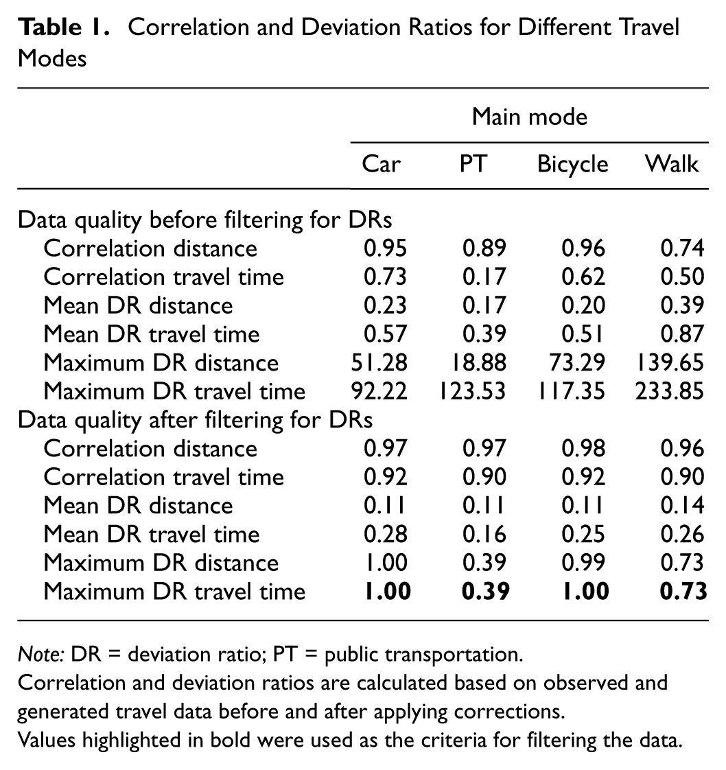
Note: DR = deviation ratio; PT = public transportation.
Correlation and deviation ratios are calculated based on observed and generated travel data before and after applying corrections.Values highlighted in bold were used as the criteria for filtering the data.
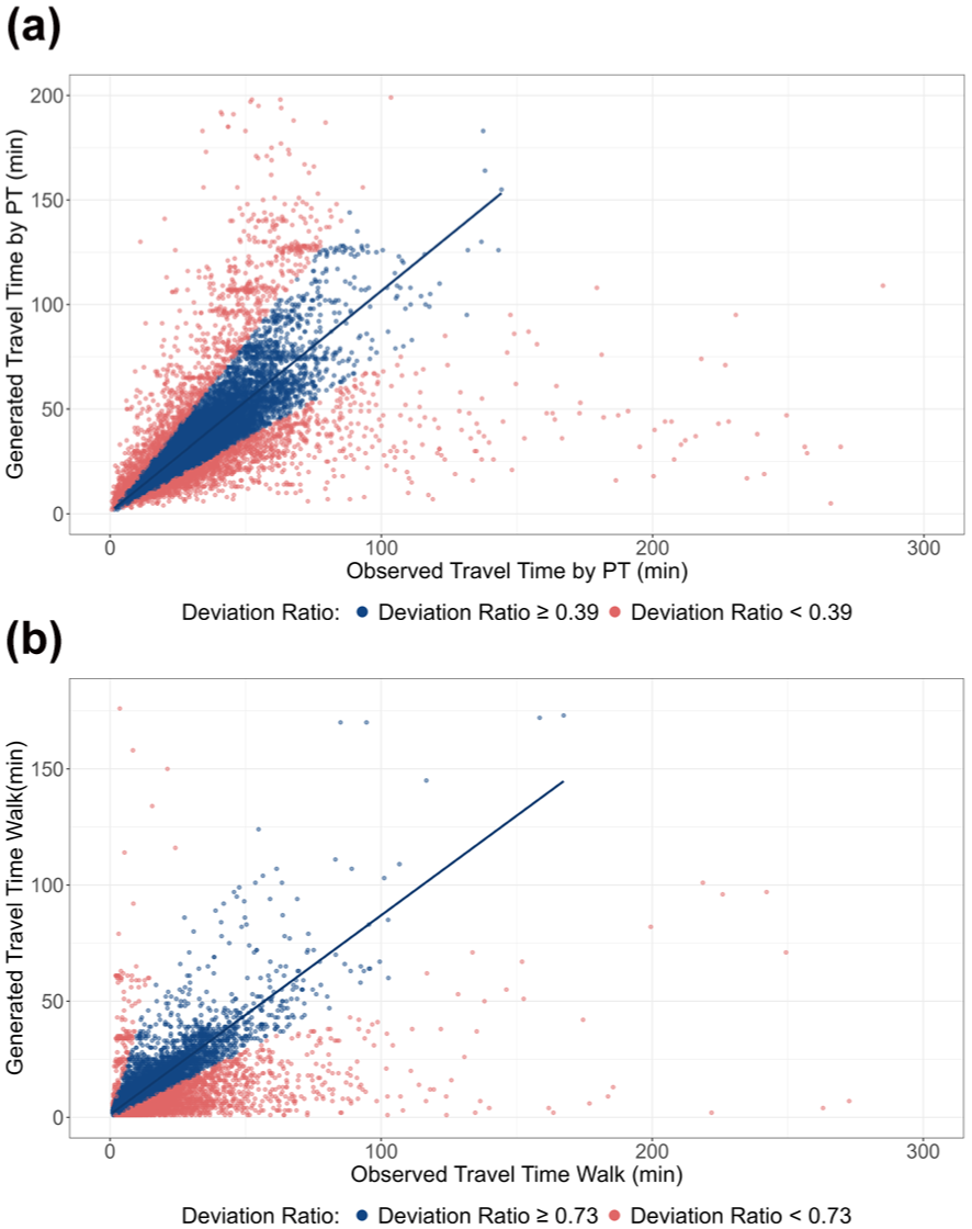
Data loss owing to filtering by deviation ratio: (a) observed versus generated travel time for public transportation (PT), and (b) observed versus generated travel time for walking.
Cost
The generated alternatives included information on mode, travel time, and distance. However, price estimation for car and PT was missing for both the observed trips and the alternatives. For bicycles, the use of shared bikes was excluded, and the cost of bicycle usage was assumed to be zero. For cars, the vehicle registration as of January 1, 2023, by the German Federal Motor Transport Authority ( 69 ) was examined to identify the 76 most common car models, which account for approximately 60% of the passenger vehicles in Germany. The average cost per kilometer for these models was obtained from Allgemeiner Deutscher Automobil Club (ADAC) ( 70 ) and weighted according to the number of cars per model to estimate a fleet-representative average price of 50.17 cents per kilometer. Similar to other studies ( 17 , 62 ), the cost calculation based on the ADAC data ( 70 ) included expenses associated with vehicle purchase, maintenance, insurance, and other long-term costs. Because of Munich’s highly complex parking system, which provides for various zones, free parking options, and parking costs that vary depending on time and location, parking fees were excluded from the cost calculation per trip. Moreover, the generally low parking costs in the city further justified their exclusion and the assumed cost of 50.17 cents per kilometer is higher than other estimates for Germany ( 71 , 72 ), accounting for additional cost burdens such as parking fees. From June to August, in addition to the 9-Euro-Ticket, the German government implemented a fuel tax cut, resulting in a 15% to 20% reduction in fuel prices ( 73 ). Accordingly, we assumed a 10% reduction in car travel costs during the intervention month of July, accounting for the per-kilometer costs including both fuel and nonfuel components, which dilute the impact of the tax cut.
A dual approach was employed for PT cost calculation. For individuals without a subscription, single-trip costs were calculated according to Munich’s fare structure (
74
) by identifying the MVV transit zones at the start and end of the trip and matching them with the corresponding costs. Other ticket options, such as day tickets, regional tickets, or stripe tickets (i.e., tickets consisting of ten strips, of which a fixed number must be validated per journey depending on distance or fare zones) available in Munich, were excluded. This exclusion introduces noise and uncertainty into the cost calculation. For those individuals with a subscription, we introduced the concept of experienced cost in which the monthly subscription cost was apportioned across the PT trips made by the individual,
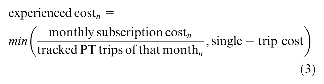
During July, the implementation of this methodology was straightforward owing to the high prevalence of individuals in the final dataset who possessed the 9-Euro-Ticket. This approach suggests that the experienced cost per trip diminishes with an increase in the number of trips made by subscription holders, thereby potentially incentivizing greater utilization of PT services to maximize the marginal benefit per trip. For September and October, determining the cost and type of subscription involved several assumptions. The respective survey only inquired about general monthly subscription ownership without specifying the exact type of ticket and its validity range. Monthly subscription prices ranged from €63 (Zone M) to €242 (Zones M to Z6) ( 74 ), making the use of a mean value unfeasible. For individuals indicating subscription ownership, the PT subscription (IsarCard) was assumed, as it is valid for all days and times throughout the month and can be purchased for specific zones, making it the most attractive option for commuters. To estimate the type of monthly subscription for a particular individual in the dataset, the most frequent MVV zones for home and work/study were calculated, and the corresponding subscription valid for these zones was assumed.
Weather
To account for the impact of weather conditions on mode choice, day- and hour-specific weather information was assigned to each trip. We utilized data provided by the German Weather Service for Munich ( 75 ), which included measures of wind speed and precipitation, as well as dummy variables indicating the presence of rain. Wind speed and minimum, maximum, and mean temperatures were recorded on a daily basis. Additionally, a rolling aggregation of precipitation effects was calculated to capture the influence of precipitation over a 3-h window. As a result of constraints in data availability, weather measurements were uniformly applied to the entire Munich area. Consequently, these measurements did not account for regional variations or microclimates within the analysis area.
Filtering Trips Through a RUM Lens
Another key challenge in utilizing GPS data for discrete choice modeling is filtering trips that adhere to rational and compensatory considerations. This behavior is predominantly observed in activity-based travel, for which individuals travel for specific purposes, primarily to meet essential needs. Consequently, this excludes recreational and pleasure trips, which follow a different logic. Differentiating between a leisurely walk with a dog, which includes a stop at a local kiosk, and a quick shopping errand is inherently complex. Various approaches have been proposed for defining mode availability and the consideration of alternatives to form the final set of choices contemplated during the decision-making process. These methodologies vary in complexity, from including probabilistic models for forming choice sets ( 76 – 78 ) to using soft cutoff terms in the utility function that constrains the availability of an alternative ( 79 , 80 ). Following a methodology similar to that employed by Tsoleridis et al. ( 17 ), we defined the consideration of alternatives in a deterministic manner with fixed thresholds as depicted in Table 2. Rather than employing data-driven or probabilistic methods, this approach relies on theoretical reasoning to establish thresholds that filter trips aligned with the analytical framework, capturing genuine economic decision-making processes. In the following section, these thresholds and their underlying reasoning will be explained. Building on and extending the work of Dahmen et al., additional thresholds were incorporated to meet the particular needs of discrete choice analysis ( 57 ). Table 2 summarizes both the thresholds adopted from Dahmen et al., as well as those newly introduced for the purposes of this study ( 57 ).
Validity Requirements for Observed and Calculated Trips
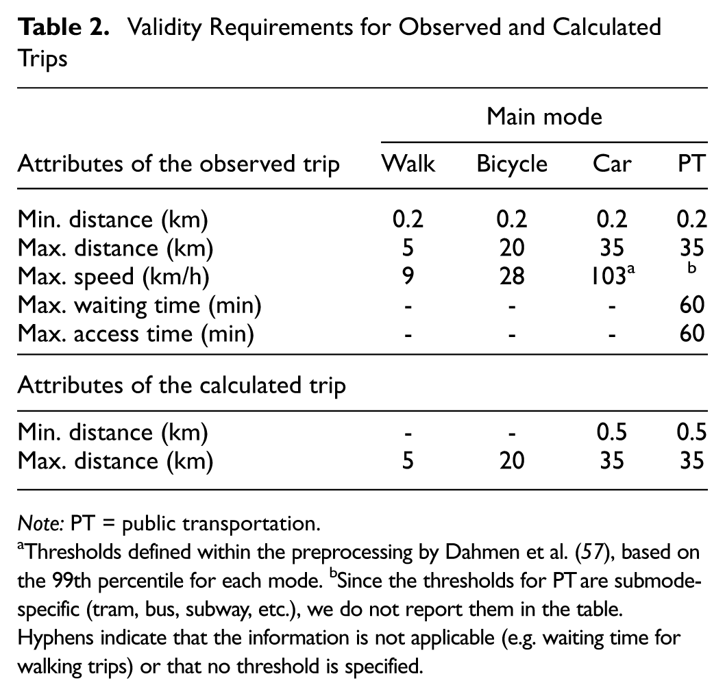
Note: PT = public transportation.
Thresholds defined within the preprocessing by Dahmen et al. ( 57 ), based on the 99th percentile for each mode. bSince the thresholds for PT are submode-specific (tram, bus, subway, etc.), we do not report them in the table.Hyphens indicate that the information is not applicable (e.g. waiting time for walking trips) or that no threshold is specified.
We included only those observed trips in the analysis that were longer than 200 m but shorter than 35 km. This constraint was chosen because trips shorter than 200 m were almost always walking trips and could have introduced noise from GPS inaccuracies. Conversely, trips longer than 35 km were sparse in the initial raw GPS dataset (as depicted in Figure 6), therefore, to avoid a few outliers having a significant impact, these were excluded. This approach also reflects the focus of the analysis on urban mobility ( 76 ) and is depicted in Figure 4 under “Distance Range.” In the Motiontag app, the trip purpose was automatically detected, but respondents had the option to change and correct the trip purpose later on ( 57 ). Purposes ranged from accompanying and medical visits to eating out. For the analysis, we grouped trip purposes into the larger categories “other,”“work/study (commuting),”“shopping,”“leisure,” and “trips toward home.” Trips labeled as other or with unknown purposes accounted for 3.7% and approximately 40% of the dataset, respectively, and were excluded owing to their high heterogeneity. The unknown trips, lacking respondent labels and automatic detection, were initially included as a separate category, but their inclusion significantly reduced model fit, reflecting high variability from their diverse, undefined purposes. The same applied to “other” trips that were highly specific in nature and represented less than 4% of the initial dataset, rendering their inclusion infeasible. This led to a crucial reduction of the dataset as depicted in the filtering step “Unknown Trips” and “Other as Purpose” in Figure 4. Trips for which no valid alternative could be calculated were excluded from the analysis, as shown in the filtering step “Valid Alternatives.” We further filtered trips for which the start and destination purposes were identical, most likely capturing strolls or unlabeled round trips. This exclusion, as shown in Figure 4 in the stage “Inconsistencies,” reduced walking trips by a significant number.
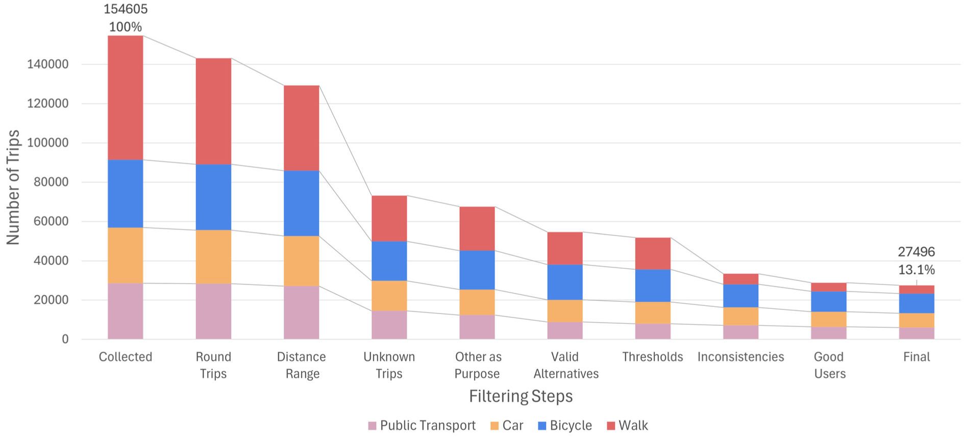
Reduction of trips as a result of filtering.
The speed of bike trips in our dataset was capped at 29 km/h, which is a reasonable speed for urban cycling. Walking trips faster than 9 km/h were excluded to eliminate running trips from our analysis. The thresholds for maximum speeds of PT and car trips originated from the preprocessing described in Dahmen et al.’s study, in which these thresholds were set at the 99th percentile for each respective submode (i.e., tram, bus, subway, etc. were considered independently) ( 57 ). Observed PT trips were excluded from the analysis if the waiting time and/or the access time exceeded 60 min to exclude disturbances. Car alternatives were included only for respondents who indicated car availability in the household survey. Similarly, bike and walk alternatives were considered only within their respective distance thresholds of less than 5 km for walking and less than 20 km for cycling, ensuring they were viable alternatives and aligned with the thresholds employed by Link et al. ( 42 ). Additionally, when computing alternative trip attributes via the APIs, car and PT trips were excluded if their routed distances were below 500 m. Consequently, car and PT alternatives were effectively only available for trips longer than 500 m in our modeling dataset. Our filtering process was mainly based on trip characteristics. The only requisite for respondents to be accounted for in the respective period was having at least 25 observed trips in the study area, depicted in Figure 4 under “Good Users.” However, we did not require participants to take trips during both periods (intervention and post-intervention). Consequently, the sample sizes for the two periods were slightly different, with 261 respondents in the intervention period and 323 in the postintervention period. Owing to July being a typical holiday month, fewer participants were recorded during this time: many respondents were traveling outside of the study area and did not reach the minimum trip threshold within the study area.
After this extensive data-cleaning process, depicted in Figure 4, only 13.1% of the initial trips were left, with 27,495 trips of 336 individuals, including 8,672 trips for July and 18,823 trips for September and October. Interestingly, the percentage of excluded trips varied significantly across modes, with only 6.7% of walking trips, 25.9% of car trips, 21% of PT trips, and 28.9% of bike trips retained. This substantial variation altered the key mode composition of the final dataset, which was crucial contextual information for interpreting the results.
Key Descriptives of the Final Dataset
A summary of the trip characteristics for each mode of the two filtered datasets is presented in Table 3. We tested whether the mean values of travel time, trip distance, and cost were significantly different between the two periods by main mode, using the Wilcoxon rank-sum test. In the final sample, individuals took an average of 2.0 trips daily, covering 12 km and 40 min of travel time per day. This was significantly lower than the MiD 2017 survey for the Munich MVV area, which reports averages of 3.8 trips, 40 km, and 95 min of travel per day ( 81 ). This discrepancy underscores that the analysis focused on a subset of daily travel, rather than the full spectrum of daily and weekly travel behavior. Notably, when examining the modal split by trip frequency of the final dataset in Figure 5, our comprehensive filtering process resulted in a mode share for which only 26.6% of the trips were made by car, 21.8% by PT, 15.3% by walking, and 36.3% by cycling. The proportion of car trips observed in our dataset was remarkably lower than the 46% reported in the MiD 2017 survey ( 81 ). Whereas the MiD survey indicated that 36% of trips were made by active modes, including walking and cycling, our final sample showed a share of 51.6% for these modes. It is important to consider that the MiD was conducted in 2017 and, therefore, does not capture the rising cycling trend and possible mode shifts resulting from the COVID-19 pandemic. Preliminary results of a mobility study in Munich ( 82 ) indicate that walking and cycling account for 55% of trips in the city in 2023 (33% and 21%, respectively). Although these reported mode shares align much closer with the ones in our final dataset, cycling accounts for more trips than walking. This could be explained by our exclusion of very short and round trips, which are often carried out on foot. Our mode share contrasts with the initial (full) Mobilität.Leben dataset, in which, as expected in observed travel data, walking trips had the highest mode share at 40.9%, followed by bike trips at 22.3%, and PT and car trips at 18% each.
Travel Metrics for Intervention and Postintervention Periods
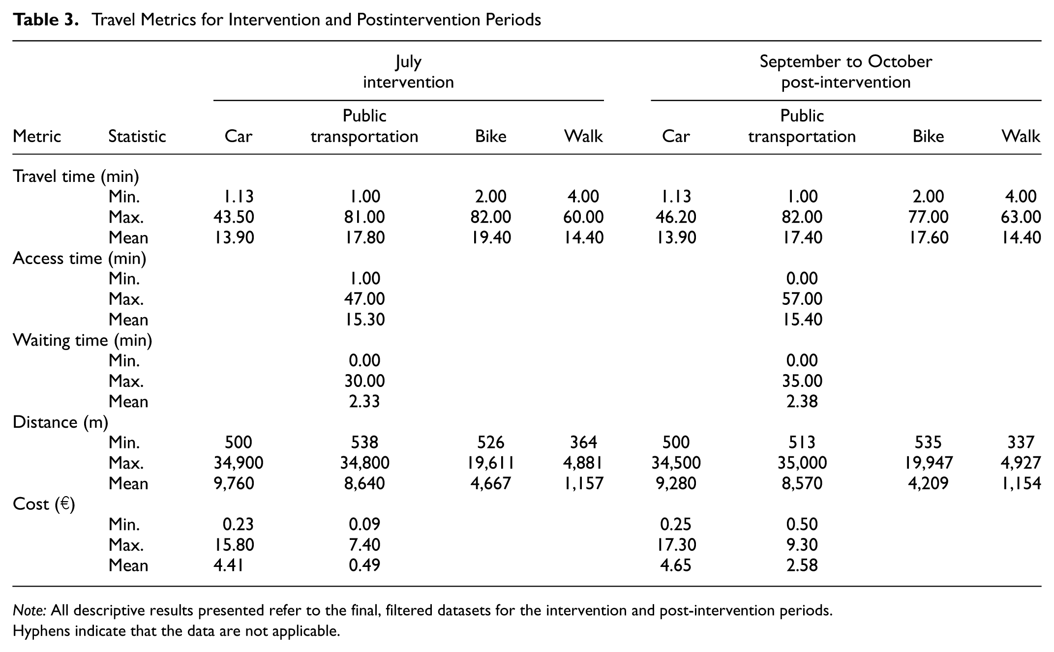
Note: All descriptive results presented refer to the final, filtered datasets for the intervention and post-intervention periods.Hyphens indicate that the data are not applicable.
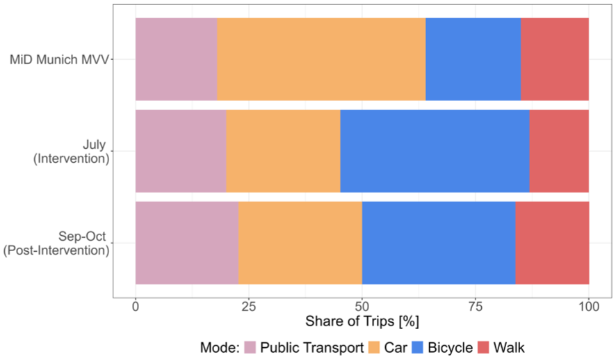
Mode share by trip frequency comparison of different datasets.
The changes in mode share by trip frequency during and after the 9-Euro-Ticket period are notable (see Figure 5). Unlike the referenced analysis on Mobilität.Leben data ( 83 ), which observed a decrease in the share of PT trips from 45.3% in the intervention period to 40.0% in September, our selected trips did not reflect this trend. The data of this analysis depicted an increase of PT usage after the end of the price intervention from 20.0% to 22.7% in September and October. We did not observe an increase in PT trips induced by the drastic price reduction in the final data sample, and any additional trips present in other studies appear to have been filtered out ( 42 , 83 ). Research suggests that the 9-Euro-Ticket increased PT usage for holiday activities and excursions ( 84 ), which do not typically fall within regular urban travel patterns. The price intervention did not seem to have increased the demand for PT trips used for daily commuting and essential short-distance travel. There was also a noticeable decrease in the share of bike trips during September to October compared with the intervention period, dropping from 41.7% to 33.8%, most likely influenced by changing weather conditions. This was also highlighted by the difference in travel times and distances for bikes during the two periods, with higher mean values in July compared with September and October. Using the Wilcoxon test the difference was significant at the 1% level. Conversely, car usage slightly increased after the 9-Euro-Ticket period, rising from 25.2% to 27.1%. This could suggest that some car trips during the intervention period were substituted by bike trips. These trends align with those observed in the referenced analysis ( 83 ).
The variation in mode share observed in the final dataset can be partly attributed to the specific subset of trips analyzed, which were filtered for short, urban distances under 35 km with a high proportion of very short trips (<15 km) favoring active transport modes, as depicted in Figure 6. In contrast, the reference data analysis included a broader dataset encompassing 670,096 trips over different periods and accounted for long-distance trips, including those by airplane ( 83 ). The MiD survey’s mode share is also constrained to the MVV area, but the share is calculated for all individual trips. Our study concentrated on a smaller subset of trips made for specific purposes (such as shopping, leisure, and commuting). When comparing the trip purposes across the two periods of analysis, as shown in Figure 7, we observed that in September and October, there was the same percentage of trips made for study and work (commuting) purposes (19.3%), but fewer trips for leisure activities (21.3%) compared with 23.0% in July. This could be explained by July being a holiday period and summer weather encouraging more leisure trips. Notably, bike trips for leisure and commuting seemed almost entirely substitued by PT trips in September and October. An unrealistically high share of trips to home was observed, most likely a result of the study setup. When respondents did not label a trip’s purpose, the app could not automatically assign it. Home had the highest share of trips overall, even before filtering, as respondents most consistently labeled this “stay”.
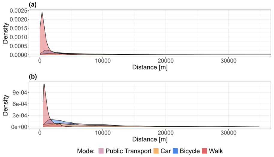
Trip distances by main mode (a) before and (b) after filtering.
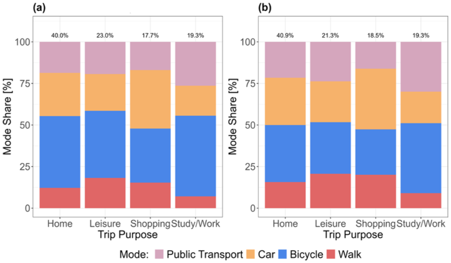
Mode share by purpose: (a) July intervention and (b) September and October postintervention.
The average experienced cost of a PT trip in July was only 49 cents (€1 = 100 cents), compared with an average of €2.58 without the price intervention (significant at the 1% level) and more than five times the mean price during the 9-Euro-Ticket period (Figure 8). Interestingly, the variance in single-trip costs for PT was markedly reduced during the postintervention period, as the maximum possible cost corresponded to the single-ticket fare. Given that regular subscription prices in September were considerably higher, observed costs remained within a narrow range around €2.58. During the intervention period, cost variance was larger, primarily owing to the pricing mechanism whereby the fixed monthly subscription fee was divided by the number of trips, causing per-trip costs to asymptotically approach zero with increasing trip frequency. For car trips, average costs were slightly lower in July at €4.41, compared with €4.65 in September and October. This reduction was marginally above the nominal 10% fuel tax cut. One plausible explanation is provided in Table 3, which indicates significantly longer average travel distances by car during the intervention period, thereby partially offsetting the artificial price reduction.
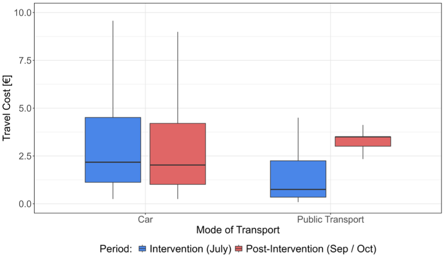
Cost distribution of car and public transport.
Overall, our sample characteristics as presented in Table 4 were not representative of the population in the region, Bavaria, in 2022 ( 85 ). A substantial proportion of the participants (62%) possessed a higher education degree, which was above the representative figure of 20%, and 11% held a PhD, a considerable overrepresentation compared with the Bavarian average of 1.6% ( 85 ). This trend was also reflected in the income levels, with 51% of participants earning €4,000 or more per month. Furthermore, the sample’s age distribution was skewed, with over 55% of participants falling within the 25- to 44-year-old age range. Notably, 89% of the sample participants reported having a 9-Euro-Ticket during the intervention period, underscoring its popularity. However, this finding is not generalizable, as a representative survey ( 51 ) found that 49% of individuals purchased a 9-Euro-Ticket in July. However, the share of subscription ownership dropped to 33% in September and October, following the end of the price intervention, probably a result of the increased travel pass cost. Close to 72% of the participants stated they had at least one car available, including ownership of a car as well as a car-sharing membership. Given the overrepresentation of young and highly educated individuals within the sample, a weighting scheme using iterative proportional fitting on the variables of gender, age, education, household size, and driver license was applied on the MNL model outcomes. This approach ensured that the VTTS estimates better aligned with population-level distributions, thus enhancing the generalizability of the findings. Importantly, the decision was made not to weight the dataset before the model estimation process. This choice reflected the priority of accurately modeling the observed data to capture the behavioral dynamics intrinsic to the collected sample, rather than introducing adjustments that could obscure the relationships present within the raw data.
Overview of the Dataset
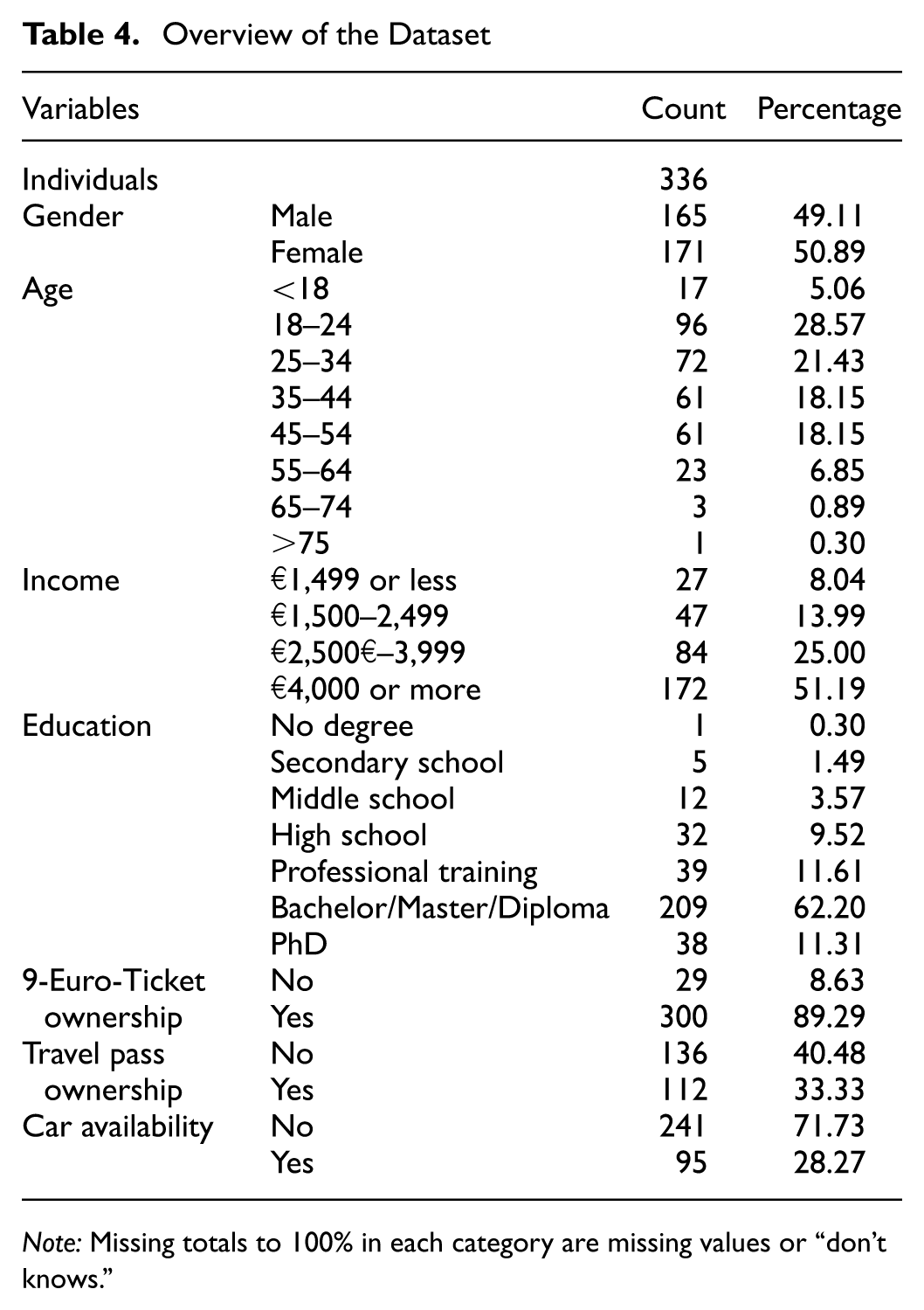
Note: Missing totals to 100% in each category are missing values or “don’t knows.”
Discrete Choice Modeling of Policy Interventions
Modeling Framework
To measure behavioral changes in mode choice resulting from price interventions such as the 9-Euro-Ticket we used the method of discrete choice modeling. Since the analyst cannot directly observe the choice process, the modeling approach utilizes the collected revealed data and assumes random utility theory (
19
,
86
). The latent utility,

For this initial exploratory analysis, the MNL was employed, chosen for its simplicity, effectiveness, and widespread use in studying mode choice in travel behavior analysis (
2
). The MNL model is based on the assumption that each

Where Vjnt denotes the deterministic utilities of alternative j in the choice set J for individual n at choice task t. The dataset is structured as panel data, encompassing multiple trips made by individuals over time. To address the dependencies inherent in such longitudinal data, the probability of choosing alternative

where
However, using an MNL model on panel data introduces certain challenges, primarily primarily due to the implications of the iid assumption. This requires that unobserved factors influencing decision making are independent across repeated choices over time. In the context of travel behavior, this can be particularly problematic as individual preferences—often not fully captured by sociodemographic variables—and state dependence, in which past choices influence current decisions, are likely to play a role in mode choice ( 1 , 87 ). Despite these limitations, the focus of this study was to provide an initial approximation of the impact of fare policy on mode preferences. Previous research has indicated that, even when the logit assumptions are violated, the MNL model can still effectively capture average taste preferences ( 1 ), making it a useful starting point for analyzing mode choice under fare policy interventions.
The Apollo package version 0.2.9 by Hess and Palma was used for the model estimation ( 88 ). To enhance the robustness of the MNL model, we employed bootstrapping with replacement, generating 30 samples at the individual level. Each sample contained the same number of individuals, and the entire modeling process was repeated for each sample. This approach ensures greater stability and reliability in the estimated parameters, addressing potential concerns with variability in the dataset.
Model Specification
There is no standardized approach in the econometric literature to accurately measure the impact of policy interventions using discrete choice models based on RP data. We identified two alternatives that could be suitable for this task.
Firstly, we estimated separate models (with observations during and before/after the intervention, respectively) and compared their postestimation results, in this case, the VTTS. A critical issue in comparing the results of two models is the scale factor. Scale factors are inversely related to the variance of the underlying datasets and are confounded with the estimated parameters ( 2 ). Therefore, the raw coefficients of the two models based on different datasets are not directly comparable ( 89 ). Fortunately, the VTTS of the two models are, since in the process of the VTTS estimation, the scale present cancels out. Thus, although the models themselves are estimated independently, the resulting VTTS values provide an interpretable basis for evaluating behavioral differences across periods.
Secondly, we tested a pooled modeling approach, combining observations from both periods and including shift variables (interactions) to capture the effect of the intervention. This is a common approach in SP studies: pricing scenarios are embedded within a single experimental design, and the data source remains homogeneous. The literature offers numerous examples of such combined models assessing pricing effects on VTTS ( 90 – 93 ). However, these typically rely on SP data or use pooled models with RP and SP data sources, which is a common and well-established practice in the literature. Pooling models based on RP/RP data have not yet been explored in depth.
In our case, such a pooled approach faced critical limitations. The two periods differed not only in the fare intervention but also in structural factors such as seasonal variation (summer versus autumn), holiday effects in July, and substantial differences in sample composition and size (8,672 versus 18,823 respondents). These factors introduce complications that could challenge the validity of a unified (pooled) model. First, size effects—where VTTS varies with the magnitude of cost/time differences—can influence estimates ( 94 , 95 ). This is a potential problem in our dataset, as the distribution of PT cost for the two time periods varied remarkably, as depicted in Figure 8. Second, an imbalance in sample sizes can skew the estimates toward the more dominant period. In our case, this would be the postintervention period. Third, whereas scale heterogeneity across periods can be modeled, this does not carry over to the VTTS, which remains confounded unless properly corrected. Lastly, there is no consensus in the literature on how best to specify the price intervention within a combined RP model. We explored several pooled model formulations, including intervention-month- and ticket-specific shifts in the alternative-specific constants (ASCs), as well as shifts in the travel time and travel cost coefficients. In addition, we specified pooled models with separate travel cost coefficients by 9-Euro-Ticket availability. We also tested specifications with period-specific scale parameters, scales by distance bands, and scales to account for differences in availability combinations across trips. However, across all specifications, the VTTS values were consistently higher, by a factor of approximately one to three, than those in the separate-period models and in comparable RP studies. This inflation occurred in both periods and may have been caused by structural differences being mistakenly attributed to the policy intervention in the pooled framework. The pooled specification imposes a single underlying utility structure and one shared error term to explain heterogeneous contexts. This may distort the resulting estimates and affect the postestimation analyses. Given these considerations, we excluded the pooled models from this manuscript. Presenting and interpreting these results would require extensive methodological discussion and contextualization, particularly with regard to the elevated VTTS values, which would go beyond the scope of this paper. Instead, we relied on separate models that, via the calculation of the VTTS, allowed a comparison between the intervention and postintervention periods.
Utility Functions
The utility functions of the two MNL models were specified for the four travel modes: car, PT, walking, and cycling. We built the model gradually by introducing each new parameter individually and testing for its performance using the log-likelihood ratio test. Each mode was associated with an ASC
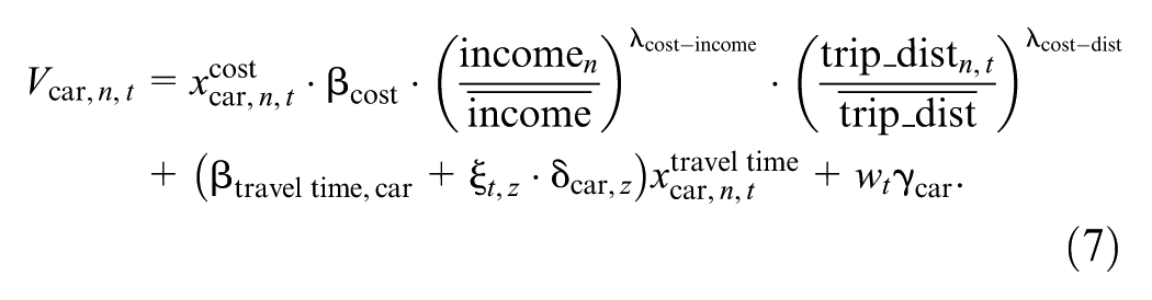
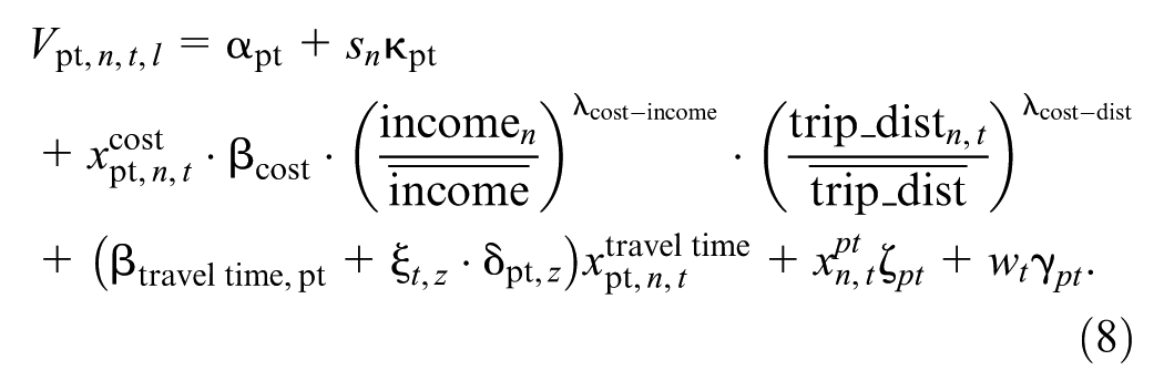
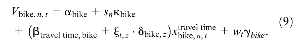
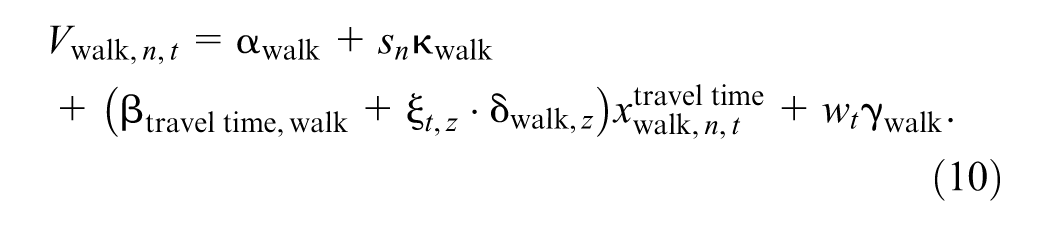
where
Although both analysis periods originated from the same data collection method, they differed significantly in participants’ travel behavior, environmental factors (such as seasonal variations and the lingering effects of COVID-19), and the presence of policy interventions. To control for sensitivities related to continuous variables, we included income elasticity,
Mode share by trip frequency of the dataset by distance.
The model estimation was carried out using a bootstrapping procedure with 30 repetitions. Importantly, whereas bootstrapping can offer a more robust inference framework by capturing sampling variability without strict distributional assumptions, the resulting confidence intervals can also be more variable and wider. In such cases, statistical significance may be harder to detect, particularly in smaller samples or complex models ( 103 , 104 ). This can lead to more conservative inferences and reduce the available statistical power to detect significant effects, which is important for the later interpretation of the findings.
Value of Travel Time Savings
An important indicator for assessing policy interventions in transportation is VTTS ( 105 ). It quantifies the willingness to pay to achieve a specific travel time reduction, thereby measuring travelers’ trade-off between travel cost and travel time ( 106 ). Equation 11 calculates, for an MNL model, the valuation of one unit (hour) of savings in time relative to one unit (euro) of change in cost.
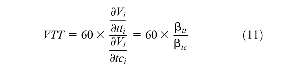
Although this standard postestimation approach uses a single ratio,
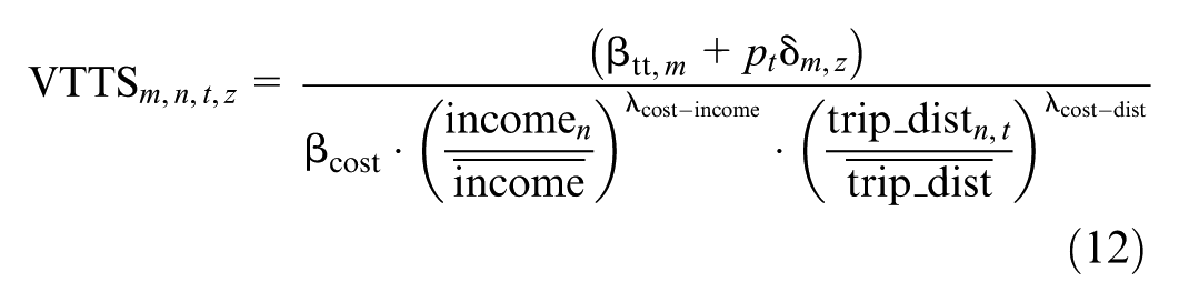
To estimate uncertainty in these values, we implemented a Monte Carlo simulation with

This simulation-based approach enabled us to incorporate sociodemographic heterogeneity directly into the VTTS estimation and to reflect the uncertainty around parameter estimates. The Krinsky–Robb method assumes joint normality of estimated parameters, which is a reasonable assumption in our case given the use of maximum likelihood estimation and a sufficiently large sample size ( 110 ). Importantly, the method does not assume symmetry in the resulting willingness-to-pay distributions ( 109 , 110 ).
Results
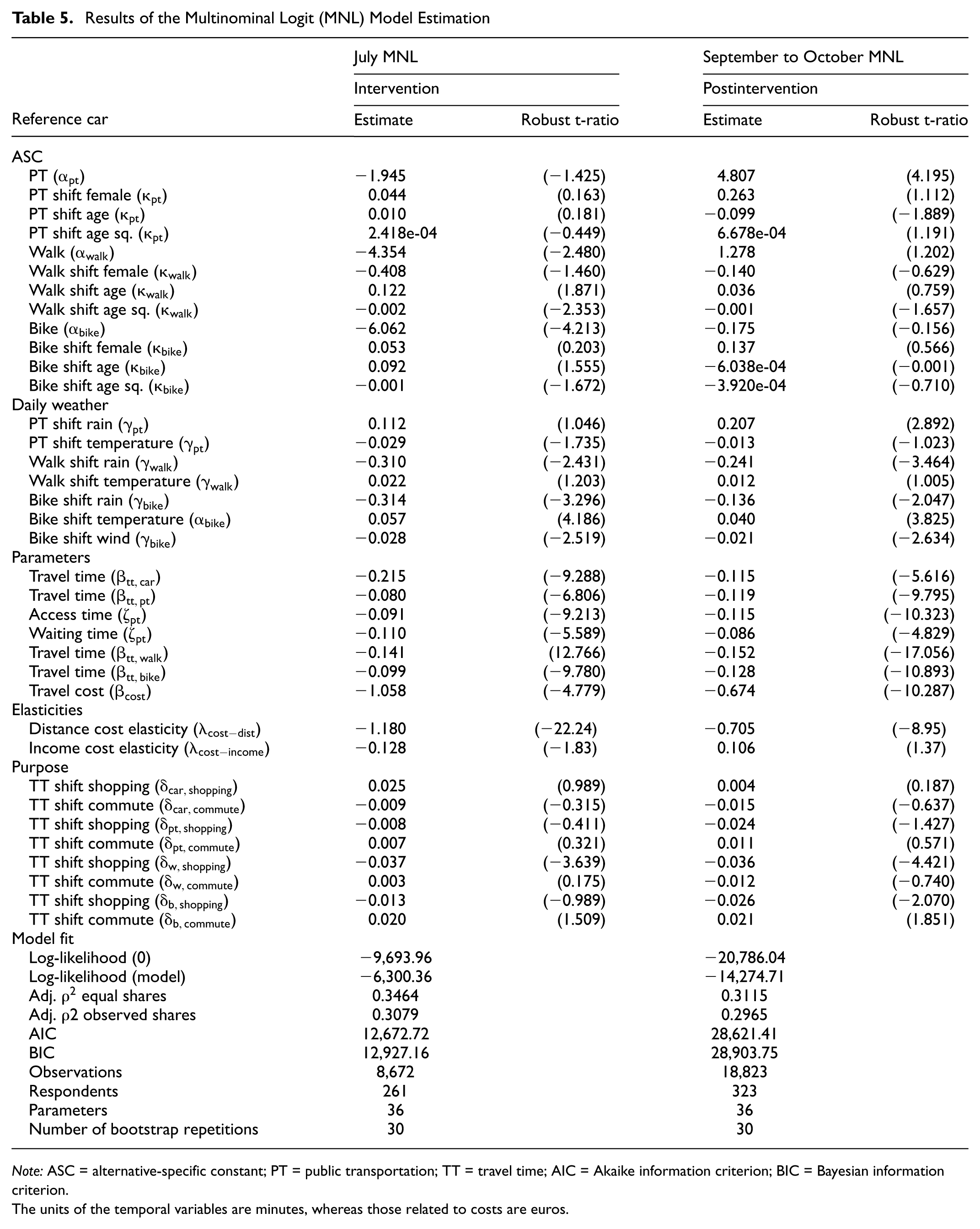
The model estimates of the two behavioral models are presented in Table 5. The July model (intervention) demonstrated superior model fit, with an adjusted (adj.)-
Results of the Multinominal Logit (MNL) Model Estimation
Note: ASC = alternative-specific constant; PT = public transportation; TT = travel time; AIC = Akaike information criterion; BIC = Bayesian information criterion.
The units of the temporal variables are minutes, whereas those related to costs are euros.
For identification purposes, one of the ASCs must be normalized to zero; in our case, this was the ASC for the car alternative. We had initially expected positive ASCs for all modes compared with the car in the July model, given the perceived favorable attitudes toward PT during the intervention period and favorable weather conditions typically promoting the use of active modes. However, in the July model, ASCs were all negative and for the active modes, even at a 5% significance level. This suggests that factors not captured by the model increased the likelihood of choosing the car, even when the model parameters were taken into account. This effect could have been caused by the still high car mode share in July (as depicted in Figure 5), despite PT fares being much cheaper during this period and favorable weather conditions encouraging the use of active modes. Thus, the reasons for people choosing the car were not present in the model and were therefore reflected in the negative ASCs.
Most sociodemographic variables were not significantly different from zero, except for the age-squared variable for walking (−0.002 and −0.001) in both models and for bike (−0.001) in the July model, for which the results were significant at the 10% level. This suggests that overall utility for walking—ceteris paribus—increased with age but decreased beyond a certain point. For PT, the age variables seemed to be unstable as they were positive for the age-squared shift, indicating that age did not affect PT usage. Similarly, the gender shifts were statistically nonsignificant. Nonetheless, we retained these shifts in the model, as it can be appropriate to include ASC shifts when their inclusion is supported by behavioral or economic theory. Taste variation is commonly captured through socioeconomic and demographic characteristics of individuals or households ( 2 , 111 ), and prior research has shown that both gender and age influence mode choice and help shape individuals’ general travel preferences ( 112 – 114 ). We therefore included these shifts in the model, but cannot draw any firm conclusions from them.
We tested various weather measurements using likelihood ratio tests and ultimately included only daily weather metrics: mean temperature, a dummy variable for rain, and maximum wind speed for cycling. Incorporating daily weather metrics led to a better model fit than hourly or aggregated weather statistics, indicating that individuals might plan their trips by incorporating daily weather information into their decision-making process. The weather-related variables showed the expected trends when contrasted with car usage. For active modes such as cycling and walking, significant outcomes were observed, with a decrease in utility when it rained. There was a significant positive effect of increased temperature on the usage of bikes at the 1% level. Similarly, strong winds significantly decreased the utility of the bike (−0.028 and −0.021) during both periods, holding all other factors constant.
As expected, the cost and travel time coefficients consistently exhibited a strong, significant, negative effect. The distance elasticity on cost was also significantly different from 1.0 and had the expected negative sign in both models. This indicated that cost sensitivity decreased as distances increased, which is behaviorally rational. Both income elasticities were significant, but revealed an ambiguous pattern. Typically, one would expect income elasticity for price sensitivity to be negative, meaning that individuals with higher incomes are less sensitive to costs, as the effective cost coefficient decreases with increasing income. This expectation held for the intervention period, during which the income elasticity was indeed negative (−0.128). However, the postintervention model exhibited a positive income elasticity, suggesting that individuals with higher incomes were more sensitive to price increases, which is counterintuitive from a behavioral perspective. We believe this result is an artifact of our method to estimate experienced PT cost, where, for individuals with a PT subscription, the total cost was divided by the number of trips taken, thereby distributing the subscription expense across all trips. Our analysis of the sample revealed that higher-income individuals were less likely to hold a PT subscription and more inclined to pay per trip, leading to higher overall and per-trip costs. This disparity in cost estimation methodology most likely explains the unexpected positive income elasticity, although further analysis would be needed to confirm this. Purpose shifts for travel time were fixed for trips with the purpose “other” and are largely nonsignificant. However, the shift for shopping walking trips (−0.037 and −0.036) showed a 1% level of statistical significance in both models. For bike, the shopping purpose shift was only significant at the 5% level in the postintervention model. These results indicated lower tolerance for longer travel durations during trips where people have to carry goods. The commuting shift was only significant at the 5% level for cycling in the postintervention model, indicating reduced sensitivity to longer travel times. This is a somewhat surprising result, as one would typically expect greater avoidance of additional travel time for highly repetitive trips like commuting, for which time losses accumulate over the course of a week. A more detailed analysis would be needed to further investigate this finding.
Overall, travel time and cost emerged as major determinants of mode choice across both models. This confirmed the central role of the trade-offs between cost and travel time in decision making. Overall, the results offered insights into the dynamics of urban travel behavior, highlighting the influence of cost and contextual factors such as weather and seasonality on mode choice preferences.
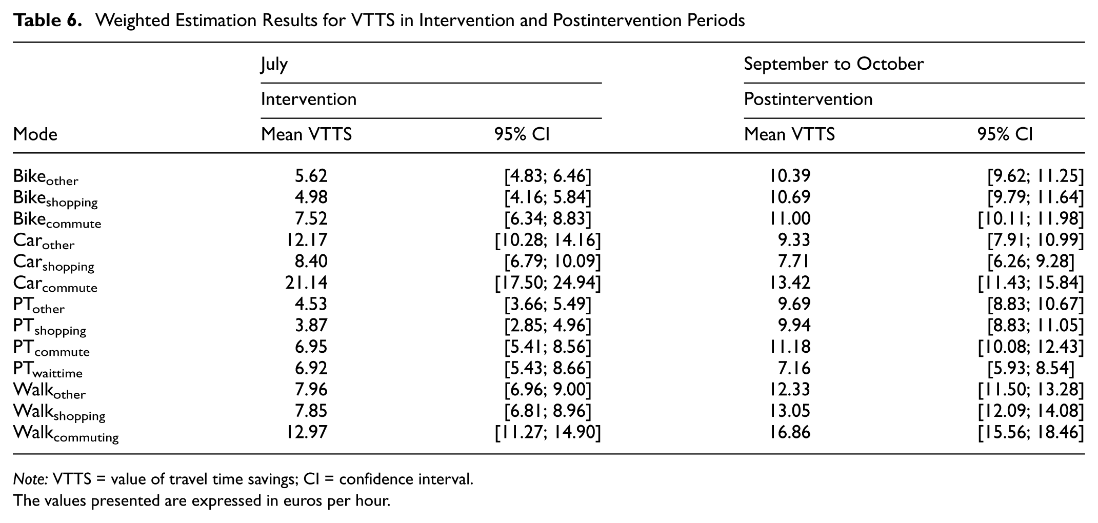
The results for the weighted VTTS, presented in Table 6, aligned with expectations. They revealed substantially lower VTTS for PT during the intervention period in July, at only €6.95/h for commuting trips compared with €11.18/h in September and October. This pattern was consistent across other trip purposes, with VTTS for PT in September and October being approximately two times higher than during the price intervention period. Overall VTTS values were also higher in the postintervention period for bike trips, showing a twofold increase compared with July, with a smaller increase for bike commuting trips. VTTS values for walking trips increased only by a factor of approximately 1.50. Higher VTTS for active modes during the postintervention period were likely to be the result of changing weather conditions, as cycling and walking became less favorable during the autumn months of September and October. In contrast, VTTS for cars decreased in the postintervention period compared with July, with €21.14/h for car commuting trips being the highest value. This is a surprising result. Potential reasons for the higher VTTS during the intervention period, which includes the fuel tax cut, could be the generally higher differences between PT and car cost. During the intervention, PT was on average the cheapest alternative compared with a car trip, as depicted in Figure 8. This means that people who still used the car were potentially less price sensitive and focused more on time efficiency than cost. This effect was exaggerated by the negative income elasticity, making high-income individuals, who were the car users in our sample, even less price sensitive.
Weighted Estimation Results for VTTS in Intervention and Postintervention Periods
Note: VTTS = value of travel time savings; CI = confidence interval.
The values presented are expressed in euros per hour.
The models revealed consistent VTTS ratios between trip purposes, particularly for commuting. VTTS for other trips was generally lower than for commuting trips, which aligns with prior findings that report higher VTTS for commuting owing to the repetitive and time-sensitive nature of such trips ( 17 , 115 ).
The observed patterns in the VTTS estimates, particularly some of the counterintuitive results, may be partly driven by the generally nonsignificant interaction effects between trip purpose and travel time. However, we decided to retain these purpose-specific shifts in the VTTS calculation, guided by the argument made by Börjesson and Eliasson ( 55 ). They emphasize the importance of capturing heterogeneity in marginal utilities across travel time components, transport modes, and trip purposes. Their findings suggest that a substantial share of VTTS variation arises precisely along these dimensions. Omitting such heterogeneity—even when interaction terms are statistically weak—risks masking meaningful behavioral differences and producing biased or overly aggregated estimates.
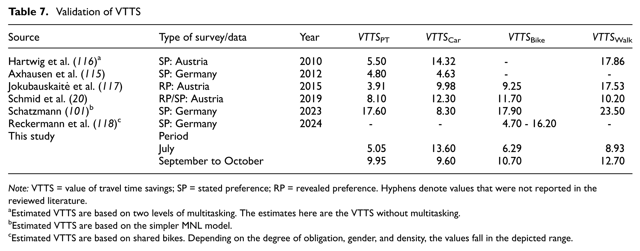
To address the problem of statistically nonsignificant purpose-specific coefficients and to enable validation with other research findings, we additionally computed weighted mean VTTS values using Equation 13. The average was calculated across trips by mode only, without incorporating purposes. Table 7 presents reference VTTS values drawn from previous studies conducted in German-speaking countries using the euro and published after 2010. The estimates of this study fell within the expected ranges reported in the literature for all modes. The only exception was the VTTS for walking in July (€8.93/h), which was slightly lower than usual values reported in the literature, ranging between €10.20 and €23.50/h. Typically, VTTS values for active modes tend to be higher, reflecting the greater effort or discomfort associated with longer walking or cycling trips. In our case, the relatively low sensitivity to walking time may be explained by Munich’s high share of active mode users. Combined with favorable weather conditions in July, walking may be experienced as more appealing and less burdensome.
Validation of VTTS
Note: VTTS = value of travel time savings; SP = stated preference; RP = revealed preference. Hyphens denote values that were not reported in the reviewed literature.
Estimated VTTS are based on two levels of multitasking. The estimates here are the VTTS without multitasking.
Estimated VTTS are based on the simpler MNL model.
Estimated VTTS are based on shared bikes. Depending on the degree of obligation, gender, and density, the values fall in the depicted range.
Importantly, even without disaggregating by purpose, the main finding held: the VTTS for PT declined substantially during the 9-Euro-Ticket period. Whether the observed increase in VTTS for car during the same period was also attributable to the policy intervention—possibly as a behavioral counterreaction—or the results stem from other factors such as weighting effects or seasonal influences, remains a question for further analysis.
Discussion
One major finding of this paper was that the hypothesis held: one could observe a significant decrease in VTTS for PT during the intervention period. The decreased VTTS translated into users’ tendency to assign a lower monetary value to time spent traveling by PT. The overall price reduction from the 9-Euro-Ticket, compared with the regular subscription price for the inner city of Munich during that time, was substantial: dropping from €63.20 per month to €9.00 ( 74 ). This has important economic and sustainability implications. First, as VTTS is a critical metric for evaluating transportation infrastructure investments, a decrease in VTTS could be interpreted as users placing less value on service improvements (e.g., reduced headways or faster connections). This could affect long-term cost–benefit assessments of PT improvements and expansion. Second, lower VTTS for PT could encourage the switch to PT as the perceived disutility of the mode decreases, thereby supporting Germany’s sustainability goal of decarbonizing transportation.
However, our research also highlights that even though VTTS are often used to understand travel patterns and are a highly important indicator for project appraisal, the calculation of VTTS exhibits important limitations. The first key challenge arises for active modes such as walking and cycling, which typically have no monetary cost. This raises the question of whether a trade-off between time and cost is behaviorally meaningful for these modes, and whether using a cost parameter based solely on PT and car costs is appropriate in VTTS estimation. This issue is not unique to our study—several experimental designs similarly lack explicit cost components for active transport. Reckermann et al. summarizes various strategies to address this ( 118 ), including relying on established monetary valuations ( 119 ) or incorporating sociodemographic and wage data to account for VTTS heterogeneity ( 120 , 121 ). Others include nonbike alternatives with cost attributes in the model to infer VTTS ( 20 , 122 ). In the absence of recent cycling-specific VTTS estimates for Munich, we adopted a generic cost parameter approach. For instance, Tsoleridis et al. derive their cost parameter from car and PT costs, yet still report a VTTS for cycling ( 17 ). A second key limitation of the VTTS estimates presented in that study is their sensitivity to methodological choices, despite aligning with figures reported in other empirical work. Unlike SP or pooled RP/SP data, GPS-RP data introduce unique challenges: high uncertainty in preprocessing, complex trip structures, and limited control over the observed choice context. These factors complicate the identification of a “true” or most realistic VTTS and contribute to the considerable spread of estimates documented in the literature on VTTS for project appraisal. Beyond methodological concerns, some researchers have also questioned the behavioral assumptions underlying VTTS itself in short-term, mode-specific decisions. Metz, for example, argues that the assumption of generalized cost minimization may be misguided, given that average travel time has remained stable over decades despite major infrastructural investment ( 123 ). He suggests an alternative framing: that travelers aim to maximize accessibility, subject to time and budget constraints, rather than minimize travel costs per se.
The third point concerns the inherent tension between two policy goals: improving equity and reducing carbon emissions by making PT more affordable or even fare-free, and the concurrent need to expand and enhance PT infrastructure, which often hinges on VTTS. When travel costs approach zero, as they might with heavily subsidized or fare-free services, standard measures of cost responsiveness and VTTS become increasingly challenging to estimate. In such cases, sensitivity to cost changes diminishes, making it unclear how to derive a meaningful “cost coefficient” for new infrastructure decisions. We suggest that planners consider whether the traditional reliance on VTTS remains appropriate in the long run, particularly when cost-based signals in PT are minimal. Consequently, our findings reinforce the view that VTTS should be interpreted as a context-dependent approximation rather than a universal or definitive measure. Transport planners and policy makers should apply VTTS estimates in concordance with other appraisal methods, such as calculating consumer surplus or other welfare indices. This could provide a clearer path for policy evaluations and infrastructural investment decisions under changing circumstances.
Beyond discussing the policy impacts of the 9-Euro-Ticket intervention, a key contribution of this paper is highlighting the critical preprocessing steps required to refine (semi-)passive travel diaries for utility-driven discrete choice models. One of the most substantial findings from this process is the extent to which trips were filtered out and the consequent implications for interpreting the results. On the one hand, filtering inherently imbalances the data, which must be considered when applying the results to other contexts. By incorporating weighting, bootstrapping, and carefully accounting for every filtering step, we have attempted to maintain the relevance of the results. Nonetheless, open questions remain about the biases introduced during preprocessing and how these might affect broader interpretations. On the other hand, the wide variability and inherent “noisiness” of urban travel behavior underscore a fundamental challenge in effectively capturing and analyzing such data. Although fine-grained data collection can yield numerous data points, its utility is limited if its accuracy, relevance, and validity cannot be ensured. Furthermore, many highly specific trip purposes and chained trip data were aggregated into broader categories to generate sufficient sample sizes and feasible alternatives. Whereas our approach enables meaningful analysis, it raises questions about future data collection strategies—specifically, how to balance the granularity of data points while ensuring their relevance and applicability for subsequent modeling and policy evaluation. One approach for ensuring accuracy could be the integration of information from other apps on the smartphone to validate and enrich the (semi-)passive travel diaries. For example, step counts, data from fitness trackers, calendar events, or energy consumption could be interesting in these contexts. The findings emphasize the importance of not only collecting detailed travel data but also ensuring their interpretability for robust applications in transportation research, cost–benefit analysis and (fare) policy assessment. This dual focus on validity and meaningfulness should guide future efforts in data collection and methodological refinement. Another limitation of our dataset arises from the absence of a dedicated preintervention period. Because our observations only covered the intervention and postintervention phases, it is difficult to ascertain whether the persistent effects of the 9-Euro-Ticket continued to influence travel behavior in the postintervention period. As such, the estimated VTTS from this later phase cannot be readily applied to the preintervention setting. Moreover, the preintervention period was characterized by additional challenges such as rising living costs without substantial relief measures, ongoing impacts of the COVID-19 pandemic, and heightened infection rates often observed in cooler months. These factors constrain the broader generalizability of our findings to a period before the 9-Euro-Ticket came into effect.
We understand that the methods applied in this study could be further enhanced in future research to better address the fine-grained and information-rich data collected. For instance, incorporating supervised machine learning techniques into the data filtering process could significantly improve the precision of trip selection and classification. One could train an algorithm on a subset of labeled trips and use such an approach on the entire data to automatically identify trips that align with our theoretical framework. Another advancement could be the inclusion of more tour-based information in the filtering process. Trip-chaining information could make the specification of final availabilities more realistic, as the current approach controls only for mobility tool ownership but not for situational availability, such as whether a privately owned car is actually at an individuals immediate disposal given preceding trips. A critical area of uncertainty in our analysis was the cost calculation for PT, given the abundance of ticket options and the difficulty in determining the actual ticket used by individuals. A limitation of this study was the inability to specify a pooled model that adequately captured the intervention effect. The pooled models consistently produced inflated VTTS estimates and showed poorer overall fit. Nevertheless, the expected effect direction—reduced VTTS for active modes and PT during the intervention period—was also visible in the pooled estimates. Although the relative size of the effect was broadly consistent, the absolute VTTS values for each period were systematically higher than those obtained from the separate models. This suggests that the intervention effect identified in the separate models was genuine, but its precise magnitude could not be reliably recovered from a pooled specification. The inability of the pooled model to produce credible results underscores the methodological challenges of incorporating substantial contextual variation within a single unified framework. Addressing these challenges requires further methodological development, which we see as an important avenue for future research, but was out of the scope of this paper. Developing a separate model to estimate the latent variable of travel pass ownership based on a broader range of variables could provide a more accurate cost assessment. We also consider that additional approaches to make VTTS comparable across studies and time periods are needed to further increase the robustness of the measures. In future research, we should try to incorporate not only observed heterogeneity through shifts and elasticities, but also random heterogeneity into the calculation of VTTS, as well as to develop approaches that account for study context and variable distribution in VTTS based on RP data. Utilizing advanced modeling techniques such as mixed logit models would allow for a more in-depth understanding of heterogeneity in travel behavior, capturing random taste variations. These advancements would lead to more accurate estimates and potentially richer data interpretations, enabling more precise policy recommendations for future research. However, estimating such mixed logit models requires careful processing of input data to ensure that the models capture genuine taste heterogeneity in choices rather than randomness introduced by inconsistencies in trip selection.
Conclusion
This study examined the impact of a fare policy intervention on the trade-offs travelers are willing to make between travel time and cost, as captured through the concept of VTTS. We achieved this objective by comparing the VTTS during and after the intervention period and by examining the estimation results. Through the comparison of the two separate models, our analysis demonstrated that the VTTS for PT during the 9-Euro-Ticket intervention in July was significantly lower than in the September to October period. This finding emphasized the substantial influence of the intervention on travel behavior, particularly its ability to lower perceived disutility associated with PT use. Moreover, our detailed data filtering and preparation process served as both a blueprint and a point of departure for future research. Although effective in deriving meaningful insights, our approach also highlights the need for further methodological advancements. We encourage greater transparency in data filtering and preprocessing when using RP data in discrete choice modeling. Such transparency is critical for enabling readers to fully understand the influence of processing steps on model outputs. Additionally, a discussion is required on advancing methods—both data-driven and theory-informed—to ensure alignment with the chosen modeling approach and to propel the field forward.
One key lesson from the presented analysis is that even with modern technologies enabling high-accuracy (semi-)passive travel diaries, the resulting data often contain a substantial proportion of “messy trips.” These trips, as described by Kent and Mulley, are spatially and temporally complex, often deviate from assumed planning behaviors, and may be emotionally or physically loaded ( 124 ). This highlights the ongoing need to refine methodologies for processing and modeling GPS-RP data, ensuring that these complexities are appropriately accounted for.
Footnotes
Acknowledgements
The authors would like to thank the TUM Think Tank at the Munich School of Politics and Public Policy for its support of the Mobilität.Leben data collection. GPT-4 assisted in debugging the R code, creating LaTeX tables, and making language edits.
Author Contributions
The authors confirm contribution to the paper as follows: study conception and design: S. Álvarez-Ossorio Martínez, F. Beck, A. Loder, K. Bogenberger; data collection: A. Loder; analysis and interpretation of results: F. Beck, S. Álvarez-Ossorio Martínez, A. Loder; draft manuscript preparation: F. Beck, S. Álvarez-Ossorio Martínez, A. Loder. All authors reviewed the results and approved the final manuscript.
Declaration of Conflicting Interests
The authors declared no potential conflicts of interest with respect to the research, authorship, and/or publication of this article.
Funding
The authors disclosed receipt of the following financial support for the research, authorship, and/or publication of this article: This research was supported by READAPT project (Grant no. 525732760) from the German Research Foundation (DFG).