Sage Journals: Discover world-class research

Abstract

The COVID-19 pandemic significantly impacted the transportation sector, altering travel demand patterns and posing challenges for local systems. Evidence of spatial heterogeneity underscores the necessity for a comprehensive understanding of these disruptions. Origin–destination (OD) matrices are generally used to compare travel patterns. Direct observations like smartphone data to construct OD matrices may limit causality in trip distribution, emphasizing the need for a methodology enabling comparison of travel patterns and exploration of factors contributing to this heterogeneity. To this end, this study develops a novel two-phase methodology. The first phase involved capturing heterogeneity in the weekly progression of zonal trip-generation patterns (via structural similarity of OD matrices) and then clustering them together based on similarity. The second phase involved examining the factors influencing cluster membership of zones. We demonstrated the proof-of-concept using two case studies: home-based work trips on weekdays and home-based other trips on weekends. The case studies focused on the Northern California Megaregion. The data used in the first phase include passively collected mobile phone data. The second phase used data on explanatory variables (e.g., mean household income, employment density, the share of white- and blue-collar workers and half-mile transit accessibility) for the multinomial logit model. This additional data to augment the data set is sourced from American Community Survey five-year estimates and the US Environmental Protection Agency. This study uniquely applies a novel methodology to two case studies, showcasing how insights into factors driving travel pattern changes can assist local and regional policymakers in optimizing resource allocation, particularly for public transportation.

Keywords

COVID-19 passively collected data OD matrices structural similarity pandemic clustering

The COVID-19 pandemic has had a profound and varied impact on travel demand patterns. The disruptive influence on demand patterns has affected local transportation system funding and caused a significant decline in revenue streams. For example, California’s local optional sales tax revenues, which support local transportation systems, experienced a decline during the initial months of the pandemic ( 1 ). Public transit systems faced severe drops in ridership and farebox revenue, and their path to recovery remains uncertain ( 2 ). At the state and federal levels, reduced vehicle usage led to a decline in fuel tax revenue, significantly impacting surface transportation funding. While the situation may have since evolved, the travel patterns did not fully return to their prepandemic state in the years following the lifting of travel restrictions ( 3 ). These lingering differences underscore the importance of understanding the shifts in travel patterns associated with disruptions during the COVID-19 pandemic. The goal is to minimize uncertainty for policymakers and transit agencies, enabling them to better plan for potential future shocks to transportation systems.

Travel demand patterns are generally analyzed using origin–destination (OD) matrices. These matrices have been used to understand the change in travel demand before and during the pandemic ( 4 , 5 ). Traditionally, the OD matrices are estimated via iterative procedures as part of the four-step transport modeling process. However, advancements in data availability now allow for the direct construction of OD matrices without the need for this iterative approach. Nevertheless, OD matrices derived solely from direct observations, such as GPS location data from mobile devices, might lack the ability to establish causality in trip distribution. This limitation becomes especially crucial when attempting to explain changes in travel demand patterns before and after specific events or interventions using OD matrices. Consequently, there arises a need for a methodology that not only facilitates the comparison of observed travel patterns (OD matrices) but also enables the exploration of the factors contributing to these changing patterns.

In this context, we propose a novel two-phase study to examine travel demand dynamics. The first phase employs a data-driven approach that uses a structural similarity metric (SSIM) to compare weekly OD matrices extracted from passively collected mobile device location data via the StreetLight platform ( 6 ). This phase focuses on exploring the continuous spatial and temporal variations in travel demand. In the second phase, a regression-based analysis is performed to further enrich the insights derived from the data-driven exploration in the first phase. Together, this methodology can enable a comprehensive understanding of travel behavior and factors contributing to observed travel patterns. We provide proof-of-concept through two case studies: home-based work trips on weekdays and other home-based trips on weekends. The data set covers the timeframe from January 2019 to October 2021, and the travel demand in 2019 acts as a reference for understanding the impact of the pandemic on travel patterns. We restricted our analysis up to October 2021 because StreetLight Data gradually changed their data sources around this period, which may impact the pre- and postpandemic comparisons. (For more details on their data sources, please read StreetLight Data [ 7 ].)

The remainder of this paper is organized as follows. The next section covers the relevant literature on efforts to understand pandemic-related disruption/recovery of travel demand using passively collected data. We then describe the data and study area, and the subsequent section provides a detailed overview of the methodology used in the study. Following is a discussion of the results, and we close the paper with a summary and conclusions, accounting for the limitations of this study.

Literature Review

The literature on the impacts of the pandemic on mobility is vast and has been the subject of multiple review articles ( 8 – 11 ). Previous studies have used various data sources and mobility indices to investigate travel behavior during and after the pandemic. Many researchers have used surveys to collect travel-related information, such as daily trip counts and vehicle miles traveled (VMT), from a sample of the population since the emergence of the pandemic ( 12 – 17 ). A benefit of administering a survey is the ability to collect detailed sociodemographic information and attitudinal responses from participants that can be used to explain heterogeneous travel behaviors at a disaggregate level. On the other hand, the travel-related information is limited to what respondents can recall from memory, which can result in unreported trips or inaccurate spatiotemporal details. Survey data are also often cross-sectional and therefore limited in their application to study changes in travel behavior over time. A travel diary survey, which involves collecting travel-related information from participants over multiple days, can overcome this limitation somewhat, and be used to study intra-individual heterogeneity. Some travel diary surveys also involve a GPS tracking smartphone app, which can more accurately record the occurrence, locations, and lengths of trips ( 18 ). However, the prohibitive costs of survey data collection and the attrition of participants generally limits the duration of a travel diary survey to one or more weeks, which precludes the study of long-term changes in travel behavior. Surveys also often suffer from sparse geographical coverage because of small sample sizes.

In contrast with surveys, direct observations of traffic counts can provide accurate estimates of continuous travel demand volume at specific locations based on measurements of every vehicle that passes the counting devices. Previous studies have used traffic count data to study vehicular emissions and air quality during the pandemic ( 19 ), or changes in nonmotorized travel activities ( 20 ), among other topics. On the other hand, these data do not include trip characteristics such as origin, destination, and trip purpose, which are important for analyzing travel demand distribution. Analyses of traffic count data are limited to aggregate flows on the instrumented parts of the road network. Traffic counts also do not capture travelers’ sociodemographic information, and it is difficult to infer such information. It is also possible that these aggregate-level metrics recovered to their prepandemic levels. However, the disaggregate travel patterns (OD patterns) did not return to the prepandemic levels or returned later. For example, super-commuting, measured as commutes over 50 mi or 90 min in one direction, has increased in many counties in California during the pandemic ( 21 ), possibly as a result of migration. It is hard to capture such changes using trip volume or VMT.

In another line of quantitative research on COVID-19’s impacts on mobility, passively collected travel data based on GPS traces from smartphones and connected vehicles is gaining popularity among researchers. The raw GPS data is collected and processed to create meaningful transportation measures. Several previous studies have used passively collected data to quantify the impacts of the pandemic on travel behavior ( 4 , 22 – 28 ). Unlike traffic count data, passively collected data can be used to generate OD matrices, allowing researchers to analyze the spatial distribution of travel demand. However, these passively collected OD matrices, derived from direct observations of human mobility, lack the ability to establish causality in changes in travel demand.

This study focuses on developing a two-phase methodology where the first phase is data-driven, and the second phase explains the factors contributing to the observed travel trends. The key idea behind the data-driven phase is the use of the structural similarity metric (SSIM) to analyze disaggregate-level OD travel patterns (trip generation) during and after the pandemic. A handful of studies in the past have explored SSIM to compare OD matrices, but they have their own limitations. For example, van Vuren and Day-Pollard ( 29 ) improved the existing method by suggesting a 4-dimensional mean SSIM that considers the Euclidean distance between OD pairs. Another approach, the geographical window-based SSIM (GSSI), introduced by Behara et al. ( 30 ), manually rearranges the OD matrices to represent local windows corresponding to geographical regions. However, the GSSI method may not fully capture the natural flow of travelers, especially when people commute long distances between counties for various reasons like affordable housing and efficient transportation. Therefore, in our study, we consider a local window based on the trip-generation pattern from a specific zone to all other zones in the study area and, by doing so, we do not miss the natural flow of travelers. Therefore, the window in the SSIM method is represented by an entire row of an OD matrix.

This paper, through two case studies, empirically analyzed weekly OD matrices for the period between January 2020 and October 2021 by comparing them with corresponding weekly OD matrices from 2019 to account for seasonality. Instead of comparing travel patterns from two time periods to understand disruption or recovery (as often done in the literature), we focused on studying the continuous weekly evolution of trip-generation patterns during the pandemic. We used a hierarchical agglomerative clustering algorithm to cluster zones with similar disruption and recovery patterns. Later, we used a multinomial logit model (MNL) to explain the cluster membership of zones, with clusters comprising the alternatives of the choice set.

Study Area and Data

We used two data sets in this study. The first data set is weekly OD matrices used to quantify spatial heterogeneity. The second data set consists of explanatory variables aggregated at the predefined zone level, which were used to learn the cause of heterogeneity. First, we provide an overview of the study area and then explain the data sets in detail in the following subsections.

Study Area

This study focused on the Northern California Megaregion, which consists of 21 counties in the San Francisco Bay area, Sacramento region, Northern San Joaquin Valley, and Monterey Bay area. The region encompasses diverse geographic characteristics and a wide range of economic activities. For example, the San Francisco Bay area has many hi-tech jobs and high average household incomes. The Northern San Joaquin Valley is more agriculture-focused and is also home to many commuters who travel to/from the San Francisco Bay area but who reside in the valley to reduce housing costs. We divided the study area into 150 Traffic Analysis Zones (referred to simply as zones in the remainder of the paper), as shown in Figure 1. The following three key considerations were considered while constructing the zone system.

Figure 1.

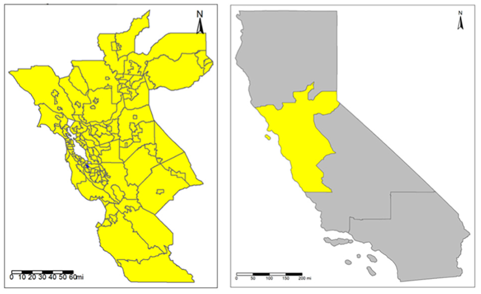
Left: zones in the study area; right: study area in the map of California.

Geographical and Administrative Boundaries

The zones in the study were created to align with county boundaries, enabling analysis of travel patterns within and between counties. At the lower level, the zones were aggregated from census tracts.

Land Use and Infrastructure

The design of the zones considered land use and infrastructure factors, influencing their shapes and sizes. Zones were clustered based on place types ( 31 ): urban, suburban, and rural, including specific areas like downtown San Francisco and downtown San Jose. Special zones were created for major transportation hubs, such as airports (Oakland, Sacramento, San Francisco, and San Jose). This approach aimed to study telecommuting patterns, remote teaching effects, and so on. We also created dedicated zones for large university campuses, enabling the potential evaluation of remote teaching and COVID-19 impacts on densely populated areas, for example, Stanford University, the University of California, Berkeley, and the University of California, Davis

Sociodemographic Information

We tried to preserve the homogeneity of sociodemographic information for census tracts within each zone. For example, income level and population were maximally kept consistent for each zone. In addition, we allocated certain zones to equity priority communities derived from Metropolitan Transport Commission (MTC) methodology ( 32 ) and SB535 criteria ( 33 ).

We also acknowledge several constraints of the defined zone system. First, we were limited to a budget of 150 zones when purchasing the data from Streetlight Data. However, it is important to cover the entire Northern California Megaregion, which enabled us to capture long-distance travel and its recovery from COVID. For example, trips between the Bay area and Sacramento region have been an important element of Northern California regional travel. As a result, each zone defined is much larger in size than traditional traffic analysis zones in the existing California Statewide Travel Demand Model. For this study, we removed three zones which represented three airports and used the remaining 147 zones for analysis.

Weekly OD Matrices

The passively collected location-based data from the StreetLight Data platform ( 6 ) from January 2019 to October 2021 was used for analysis. The StreetLight Data has been used in several studies to understand the impact of the pandemic on travel ( 23 – 26 , 34 ). The OD matrices were available for different periods of the day, day of the week, and trip purpose. The two types of days are: a typical weekday (average of daily OD values from Monday to Thursday, excluding Fridays) and a typical weekend (average of OD values from Saturday and Sunday). The unit of analysis was the estimated average daily OD trip volume.

StreetLight Data also infers travelers’ home and work locations based on their device’s location during night times (7 p.m. to 8 a.m.) and during the daytime (11 a.m. to 4 p.m.) on weekdays. (For more details on the methodology to infer home and work location, please refer to StreetLight Data Support [ 35 ].) The NextGen National Household Travel Survey Passenger OD Data products also classify home and workplace locations in a similar way ( 36 ). The home and work location together are used to deduce the purpose of each trip. The two types of trip purposes used in the two case studies are:

Home-based work trip: trips between home and work location.

Home-based other trip: trips between home and non-work locations such as grocery stores.

Data for Explanatory Variables

The data used to create explanatory variables for the MNL came from the 2019 American Community Survey (ACS) 5-year estimates, the United States Environmental Protection Agency (EPA) Smart Location Database ( 37 ), and the California Department of Public Health (CDPH) COVID-19 Vaccine Progress Dashboard. We also used the share of the population in a zone belonging to equity priority tracts (as derived from MTC methodology [ 32 ] and SB535 criteria [ 33 ]). We downloaded version 3.0 of the Smart Location Database and used the tidycensus R package ( 38 , 39 ) to download variables from the ACS. From the CDPH, we downloaded the most recent data on COVID-19 vaccines administered by demographics and by county as of July 25, 2023 ( 40 ). While the Smart Location Database variables are only defined at the census block group level (CBG), we were able to extract ACS variables at the census tract level. Table 1 lists the variables we extracted from these data sources.

Table 1

Explanatory Variables Extracted from the 2019 American Community Survey (ACS) 5-Year Estimates and the United States Environmental Protection Agency Smart Location Database

Raw variables	Explanatory variables used in MNL
ACS
Total population (census tract)	Population density
Household income in the past 12 months (in 2020 inflation-adjusted dollars)	Mean household income
Total employed in the civilian (resident) labor force for the population 16 years and over	Employment density
Industry for the civilian (resident) employed population 16 years and over	Share of white- and blue-collar workers
Smart location database
Total land area that is not protected from development	Half-mile transit accessibility
The proportion of CBG employment within ½ mi of fixed-guideway transit stop	Half-mile transit accessibility
Total land area	Multimodal road density
Road network density in facility miles of multimodal links per square mile	Multimodal road density
Vaccine progress dashboard
Administered date	Months for the county to reach 50% vaccination
Estimated population (of age group in the county)
Cumulative fully vaccinated

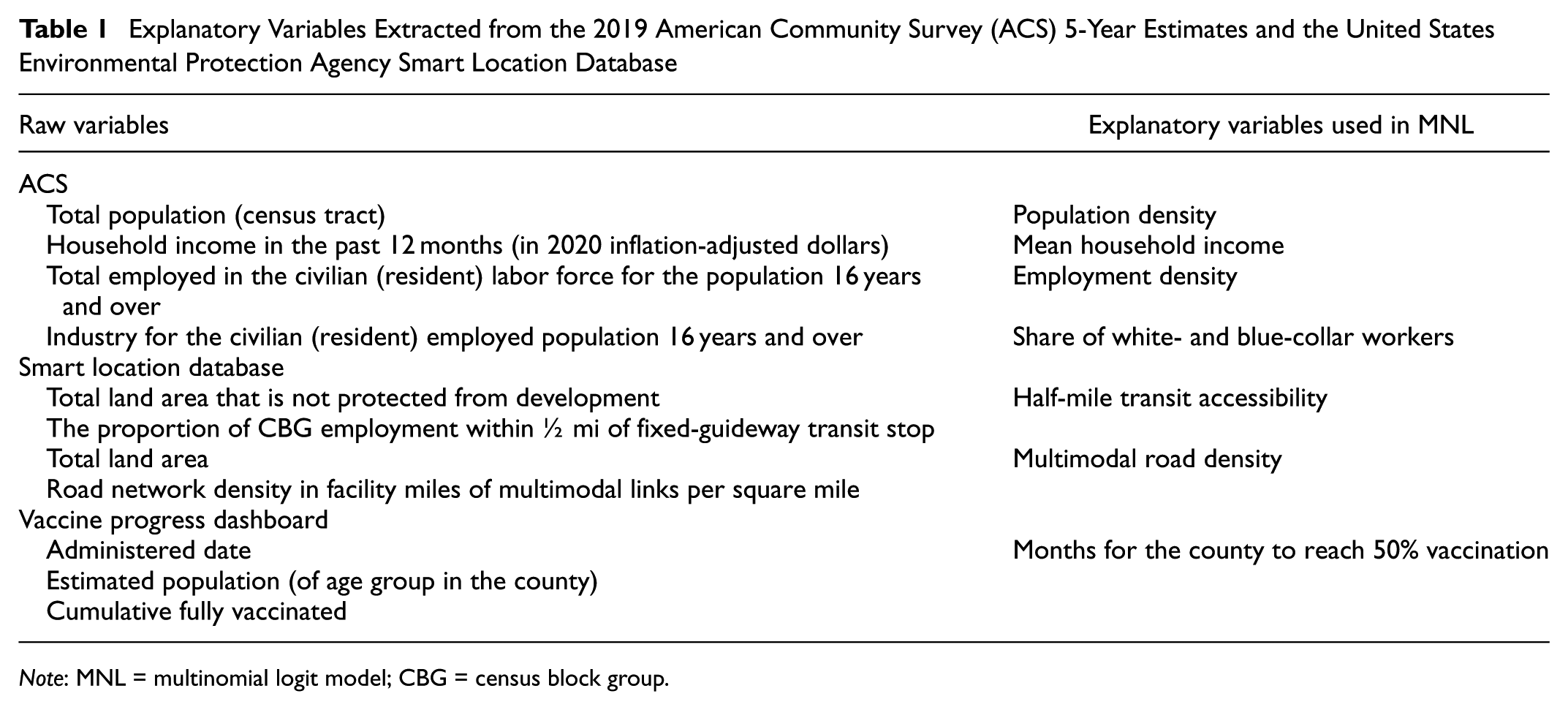
Note: MNL = multinomial logit model; CBG = census block group.

We processed the raw variables in Table 1 to derive new variables. The household income variables provide the estimated number of households within a census tract that fall into each of the 16 income groups, ranging from less than $10,000 to $200,000 or more. For each census tract, we computed the average household income as the weighted mean of the middle values of each income range, using the household estimates as weights. We also grouped industries in which the census tract residents are employed into white-collar and blue-collar categories. White-collar industries include information; finance and insurance; real estate; rental and leasing; management of companies and enterprises; professional, scientific, and technical services; administrative, waste management, and other services; and public administration. Blue-collar sectors include agriculture, forestry, fishing, and hunting; mining, quarrying, and oil and gas extraction; utilities; construction; manufacturing; wholesale trade; transportation and warehousing; and retail trade. The Smart Location Database estimates the proportion of CBG employment accessible to a fixed-guideway transit as the ratio of the area of unprotected land within one-half mile (crow-fly distance) of a fixed-guideway transit stop to the total unprotected land area. Therefore, before aggregating the transit accessibility variable to the zones in our study area, we first multiplied the transit accessibility variable by the area of unprotected land to get the area of land accessible to transit in each CBG. Similarly, the road network density in facility miles of multimodal links per square mile is estimated as the ratio of the total facility miles to the total land area. The definition of multimodal road facilities is based on the attributes of road links including speed category, number of lanes, direction of travel, and auto and pedestrian restrictions. Multimodal road facilities accept travel by both auto and pedestrians. (For more information about the Smart Location Database variables, please see their technical documentation [ 41 ].)

Next, we aggregated the data to the 147 zones in our study area. To calculate the population and employment densities of each zone, we summed the constituent census tract populations and employment numbers. We divided the results by the total area of the zone in square miles. For household income in each zone, we computed the weighted mean from the average household incomes of the constituent census tracts using the total number of households as weights. We calculated the shares of white- and blue-collar workers in each zone by summing the counts of each type of worker across the constituent census tracts and dividing the results by the total of employed residents. The Smart Location Database variables had to be aggregated from the CBG level to the zone level. After combining the transit-accessible land areas to obtain the total area for each zone, we divided the total area of land accessible to transit by the total area of unprotected land for each zone to retrieve the estimated proportion of employment within one-half mile of a fixed-guideway transit stop.

From the earliest date in the CDPH data when vaccines were administered in any of the counties of interest, for each county, we calculated the number of months until the percentage of people under 65 who had completed the primary vaccination series passed 50%. We excluded people 65 and older because this segment of the population was prioritized for vaccine administration and would introduce a systemic bias to the data. For each zone in the same county, we assigned to each of them the number of months for that county to reach 50% vaccination coverage in the population under 65, as the data were available at the county level.

Methodology

The methodology utilized in this paper consists of two primary components, as shown in Figure 2. First, we examined the spatial-temporal variation in trip generation at a disaggregate level for different zones. The SSIM concept, especially the consideration of the entire OD row as a local window, is based on trip generation, which adds value to our methodology (more details about SSIM are discussed in the subsequent section). Next, we employed agglomerative hierarchical cluster analysis to group zones with similar continuous temporal variations. In the second component, we delved into understanding the reasons behind these clusters using multinomial logit model (MNL).

Figure 2.

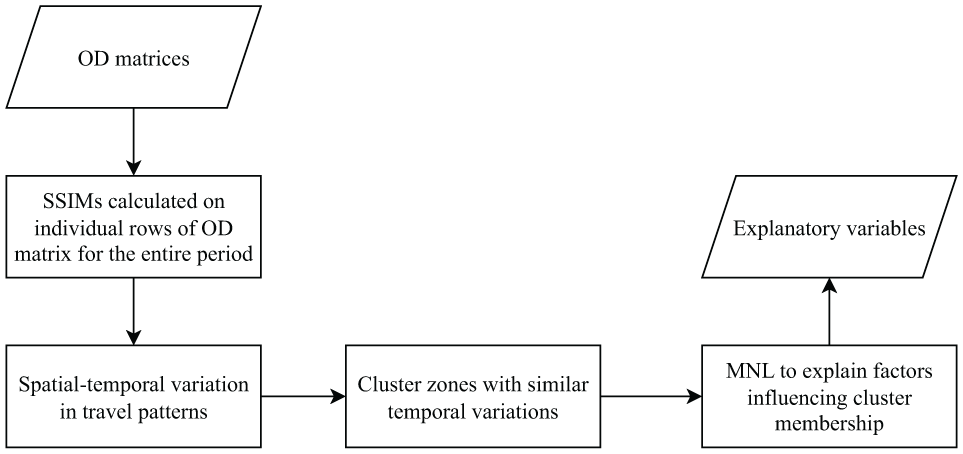
Conceptual diagram of the study methodology.

Trip Generation-Based Window for SSIM

Although OD flow primarily provides two-dimensional information concerning the trip origin and destination, the structure of an OD matrix (or a segment of it) can offer valuable insights into the distribution of travel patterns. Recent studies have been dedicated to developing methods that capture this additional information through SSIMs ( 30 , 42 – 44 ). The SSIM represents the structural similarity between submatrices of two OD matrices, a measure of similarity that accounts for correlations between different OD pairs. The SSIM is a product of three components that correspond to the mean $(L)$ , standard deviation $(C)$ , and coefficient of correlation ( $STR$ ) between groups of OD pairs as shown in Equations 1 to 5:

L (x_{w}, {\hat{x}}_{w}) = \frac{(2 μ_{x_{w}} μ_{{\hat{x}}_{w}} + C_{1})}{(μ_{x_{w}}^{2} + μ_{{\hat{x}}_{w}}^{2} + C_{1})}

(1)

C (x_{w}, {\hat{x}}_{w}) = \frac{(2 σ_{x_{w}} σ_{{\hat{x}}_{w}} + C_{2})}{(σ_{x_{w}}^{2} + σ_{{\hat{x}}_{w}}^{2} + C_{2})}

(2)

STR (x_{w}, {\hat{x}}_{w}) = \frac{(σ_{x_{w} {\hat{x}}_{w}} + C_{3})}{(σ_{x_{w}} σ_{{\hat{x}}_{w}} + C_{3})}

(3)

\begin{matrix} SSIM (x_{w}, {\hat{x}}_{w}) = [L {(x_{w}, {\hat{x}}_{w})}^{α}] [C {(x_{w}, {\hat{x}}_{w})}^{β}] [STR {(x_{w}, {\hat{x}}_{w})}^{γ}]; \\ α > 0, β > 0, γ > 0; \end{matrix}

(4)

[- 1 \leq SSIM (x_{w}, {\hat{x}}_{w}) \leq 1]

(5)

where $x_{w}$ represents an OD submatrix for a week in 2019 and ${\hat{x}}_{w}$ represents a corresponding OD submatrix for the same week between January 2020 and October 2021; $L (x_{w}, {\hat{x}}_{w})$ and $C (x_{w}, {\hat{x}}_{w})$ compare the mean values and standard deviations of the submatrices; and $STR (x_{w}, {\hat{x}}_{w})$ computes the coefficient of correlation and thus compares the structure of the submatrices. The coefficients $α$ , $β$ , and $γ$ in Equation 4 can be used to adjust the relative importance of each component and is generally set to 1. The constants $C_{1}$ , $C_{2}$ , and $C_{3}$ provide mathematical stability and are set to small values. The values of $C_{1}$ and $C_{2}$ were set to 10⁻¹⁰ and 10⁻², and $C_{3}$ was assumed to be $C_{2}$ /2 as mentioned in previous studies ( 45 ).

In this study, we propose to consider the entire row of an OD matrix as a local window for SSIM calculation. By considering trips generated from a specific zone (entire row of an OD matrix) to all other zones in the network, we capture the natural movement of travelers.

Spatial-Temporal Variation in Trip Patterns

In this study, we compared the weekly trip-generation patterns of each zone in the study area for the period between January 2020 and October 2021 with corresponding weeks in 2019 to account for seasonality. The resulting time series of a SSIM curve captured the temporal variations in the trip-generation patterns of a zone. The variation among these curves represents the spatial heterogeneity in disruption and recovery among zones. These 147 SSIM time-series curves were clustered using an agglomerative hierarchical clustering algorithm. Each cluster represented zones with similar temporal patterns in the disruption and recovery from the pandemic. We conducted the entire exercise for two kinds of OD matrices: 1) home-based work trips on a typical weekday; and 2) home-based other trips on a typical weekend.

Agglomerative Hierarchical Clustering

The SSIM curve of each zone consists of weekly SSIM values between January 2020 and October 2021. The 147 SSIM curves (each curve/observation is very high dimensional) were grouped using the agglomerative hierarchical clustering technique. We used the stats package in R ( 46 ) for clustering. We used “Euclidean” distance to compute the distance matrix and later tried different agglomeration (linkage) methods. Ward’s minimum variance method suggested the strongest clustering structure and was used in further analysis. Based on judgment and several trials, we decided to use three clusters in the study.

Multinomial Logit Model

The objective of this study is to explore the factors influencing the heterogeneity in disruption and recovery during and after the pandemic. The membership of a zone to one of the clusters, each of which represents different levels and rates of disruption and recovery, depends on multiple factors. Therefore, we specify a MNL of cluster membership. Equation 6 shows the probability, $P_{ni}$ , then zone $n$ belongs to cluster $i$ :

\begin{matrix} P_{ni} = \frac{\exp (β_{i}^{'} x_{n} + k_{i})}{\sum_{j = 1}^{J} \exp (β_{i}^{'} x_{n} + k_{j})}, \end{matrix}

(6)

where $x_{n}$ is a vector of explanatory variables for zone $n$ ; $β_{i}^{'}$ is a vector of coefficients for cluster $i$ ; $k_{i}$ is a constant parameter specific to cluster $i$ ; and $J$ is the number of clusters. The explanatory variables include mean household income (in thousands of dollars), the population density per square mile, and employment density per square mile. They also include the shares of working residents in the zone employed in white- and blue-collar industries. To account for the effect of transit accessibility, one explanatory variable is included, which represents the proportion of employment within one-half mile of a fixed-guideway transit stop. In addition, the density of multimodal road facilities per square mile is included to account for differences in connectivity and urban design between zones. We also include time taken (in months) for 50% of people aged under 65 in a zone to complete the initial COVID-19 vaccination series. Finally, we include the percentage of the zone population that lives in an equity-priority community. We used the Apollo R package ( 47 ) to estimate the MNL.

Results

This section discusses the results for disruption and recovery of two types of trip purposes: home-based work trips on a typical weekday and home-based other trips on a typical weekend. The zones with similar responses to the pandemic were clustered, and later, MNL was employed to explain the factors influencing cluster membership. The detailed results are presented in the following two subsections.

Spatial-Temporal Variation of Travel Demand

The SSIM curves are created for each zone for both analyses separately. The curves were then clustered into three groups. Figures 3 and 4 show the three clusters of SSIM curves in both analyses. The first cluster (in yellow) is named “minimum impact,” and it represents the zones that experienced the least disruption and fastest recovery. The second cluster (in blue) is named “intermediate impact,” and it represents the zones that experienced more disruption and slower recovery. The third cluster (in red), named “maximum impact,” represents zones that experienced the most disruption and late recovery. The left plot of Figures 3 and 4 shows the width of clusters, represented using different colors. The width of a cluster at any given week represents the minimum and maximum value of the middle 80% of the SSIMs of that week. The middle 80% of SSIMs are used to avoid overlapping clusters and for better visualization. The right plots show the zones in the study area colored by their cluster membership, allowing us to visualize them better. Detailed discussions of both trip purposes are presented in the next subsection.

Figure 3.

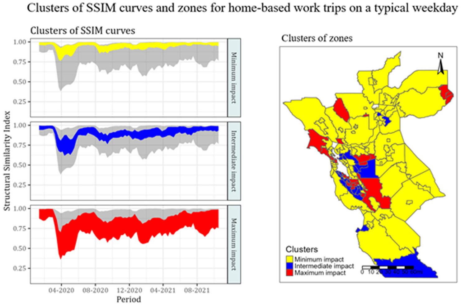
Clusters of SSIM curves based on home-based work trips on a typical weekday.

Figure 4.

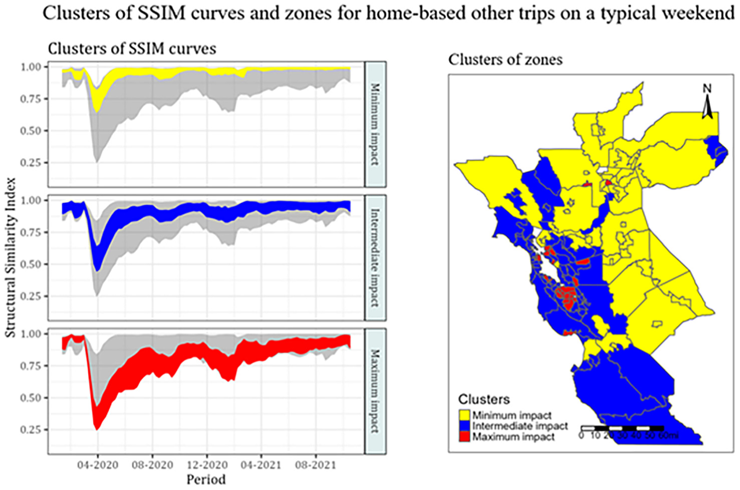
Clusters of SSIM curves based on home-based other trips on a typical weekend.

Please note that the SSIM values lie between −1 and 1, where 1 represents the OD matrices that are perfectly similar, and −1 presents the maximum dissimilarity between them. The SSIM values do not have an intuitive meaning, and the study only observed the variation among SSIM curves to demonstrate the heterogeneity in the disruption and recovery of travel demand.

Home-Based Work Trips on Weekdays

Home-based work trips represent trips whose one trip end is home and another trip end is the workplace. The home-based work trips on weekdays are mainly responsible for congestion during peak a.m. and peak p.m. A better understanding of spatial-temporal variations of home-based work trips is essential for traffic management centers and transportation planners to allocate limited resources optimally to manage congestion, and so on. Out of 147 zones, 94 zones were in the “minimum impact” cluster and experienced the least impact, 23 zones were in the “intermediate impact” cluster, and the remaining 30 zones were in the “maximum impact” cluster. The ribbon plot of the “maximum impact” cluster is wider than other clusters and shows higher volatility. It also highlights that the trip-generation patterns have not returned to the prepandemic patterns in the “maximum impact” cluster by the end of the study period. In comparison, the other two clusters seem to have nearly returned to the prepandemic levels by October 2021. The left plot also shows that the first two clusters had some recovery during June 2020 and later experienced minor disruptions during the subsequent waves of the pandemic. On further investigation, we observed an unexpected decline in trip volume in June 2019. Therefore, trip-generation patterns of June 2020, when compared with those of June 2019, give an impression of some recovery. We suspect the recovery in June 2020 is caused by an issue in the data.

The right image in Figure 3 shows the cluster membership of the zones. The rural zones in the east, north, and south sides of the study (mainly characterized by the large size of the zone) belong to the “minimum impact” cluster and have experienced the least disruption and quicker recovery. While many zones in the San Francisco Bay area (in the west) belong to the “intermediate impact” or “maximum impact” cluster, indicating these zones experienced a larger impact of the pandemic. These zones also have higher proportions of white-collar employees who could opt for remote work. For example, the city of Davis, which is a college town and home to the University of California Davis also belongs to “maximum impact” cluster, possibly because universities continued to operate in remote/hybrid mode during the study period. Some zones in Sacramento, the capital of California, also belong to the “intermediate impact” cluster, possibly the result of the higher share of white-collar employees.

Home-Based Other Trips on Weekends

Home-based other trips represent trips whose one trip end is home, but the other trip end is not a workplace. For example, a trip from/to home to/from the grocery store or gym. The home-based other trips on weekends constitute a significant proportion of the weekend trip volume. The SSIM curves were clustered into three groups based on the zonal level response to the pandemic. Out of 147 zones, 57 zones are in the “minimum impact” cluster and experienced the least impact, 66 zones are in the “intermediate impact” cluster, and the remaining 24 zones are in the “maximum impact” cluster. As is visible from Figure 4, the SSIM curves of home-based other trips on weekends experienced relatively higher disruption than home-based work trips on weekdays during the early phase of the pandemic. This is possibly because of the closure of businesses, stay-at-home orders, and so on. The trip-generation patterns of the zones in the “minimum impact” cluster recovered quickly after the first wave of the pandemic, followed by zones in the “intermediate impact” cluster. The zones in the “maximum impact” cluster recovered quite late but were less volatile than the corresponding cluster in the home-based work trip. The right plot in Figure 4 shows the cluster membership of the zones. A larger proportion of zones belonged to the “intermediate impact” or “maximum impact” cluster, mainly covering the Bay Area, parts of Sacramento, the city of Davis, Napa, Marin, Monterey, and San Benita Counties.

Multinomial Logit Model Results

The second phase of the proposed methodology includes the MNL to explain the factors influencing cluster membership of each zone for both analyses. The explanatory variables used in the model were described in the methodology section and were presented in Table 1. The estimates of MNL models are shown in Table 2. The first model explains home-based work trips on weekdays, and the second model explains home-based other trips on weekends.

Table 2.

Results of selected Multinomial Logit Models for Home-Based Work Trips on Weekdays and Home-Based Other Trips on Weekends

Trip purpose	Home-based work trips on weekdays			Home-based other trips on weekends
Number of zones in each cluster	94	23	30	57	66	24
Clusters	Minimum impact	Intermediate impact	Maximum impact	Minimum impact	Intermediate impact	Maximum impact
Constant	~	−4.79*	−0.73	~	3.83	3.76
Mean income (in thousands)	~	0.05**	0.04**	~	0.04**	0.06**
Population density (in thousands)	~	−0.13	−2.82**	~	−3.16**	−3.85**
Employed resident density per sq. mile (in thousands)	~	−0.03	4.34**	~	6.61**	7.74**
Share of resident white-collar workers in a zone	~	2.29	0.92	~	−5.63	−8.10
Share of resident blue-collar workers in a zone	~	−11.63**	−9.10	~	−5.87	−17.91**
Half-mile transit accessibility index	~	−0.26	−4.91*	~	5.87	4.02
Months to reach 50% Vaccination rate	~	−0.05	−0.21	~	−0.31**	−0.39**
Percent of equity-priority community residents	~	0.05**	0.02	~	0.01	0.05*
Multimodal road density	~	0.32	1.07**	~	−0.52	0.2
Adjusted-Rho-squared versus equal shares	0.33			0.32
Adjusted-Rho-squared versus observed shares	0.19			0.29
AIC	212.74			215.14
BIC	272.14			274.54

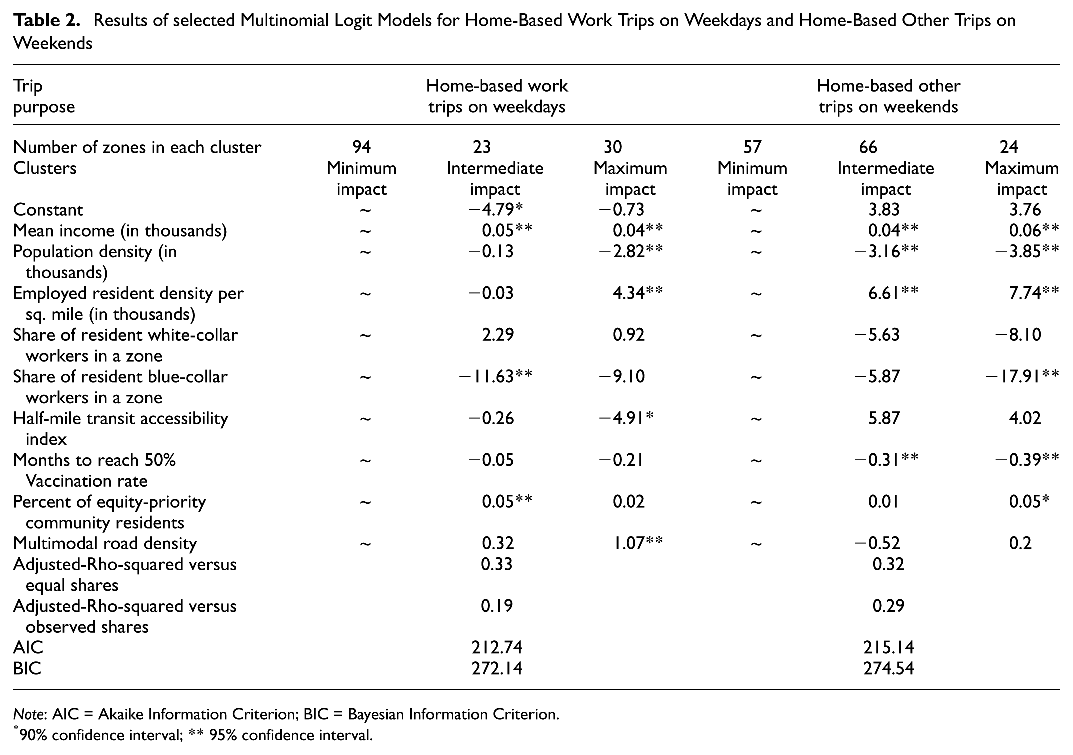
Note: AIC = Akaike Information Criterion; BIC = Bayesian Information Criterion.

90% confidence interval; ** 95% confidence interval.

The results suggest that the mean household income of a zone is positively associated with belonging to the cluster of zones that experienced intermediate or maximum disruption and slow recovery. As can be seen from Figure 3, most high-income zones in the Santa Clara Valley and East Bay areas, and to the northwest of downtown San Francisco, experienced an intermediate or maximum impact of COVID-19 on the generation of these trips. Population density was found to be negatively associated with both models’ maximum impact cluster of trips. Taken together, these results are consistent with the idea that higher-income households tend to be in less densely populated areas where travel patterns were not as greatly impacted by the COVID-19 pandemic.

On the other hand, the density of employed residents per square mile is positively associated with the maximum impact cluster of trips in both models. This may be explained by businesses closing or transitioning to telework after the onset of the COVID-19 pandemic and employees reducing expenditure on travel because of income security concerns. The share of blue-collar jobs in a zone is negatively associated with the intermediate impact cluster of home-based work trips on weekdays, and the maximum impact cluster of home-based other trips on weekends; which may be explained by blue-collar workers being less likely to transition to telework or e-shopping. The vaccination rate was negatively associated with intermediate or maximum impact clusters as expected. The percentage of equity-priority community residents in a zone is positively associated with the intermediate impact cluster of home-based work trips on weekdays and the maximum impact cluster of home-based other trips on weekends.

Several explanatory variables, such as the half-mile transit accessibility index and the share of white-collar workers, were insignificant, suggesting they did not influence the cluster membership. It is likely that 1) a small sample size of 147, 2) the dilution of explanatory information during aggregation from census blocks/tracts to the predefined zones, and 3) the correlation between explanatory variables limited the ability of the models to explain the factors effectively. However, the two case studies provide validation of our proposed novel approach, firmly establishing its proof-of-concept.

Summary and Conclusion

While OD matrices derived from passively collected data present exciting opportunities for transportation demand analysis, they lack causality in trip distribution. This study addresses this limitation by introducing a novel two-stage methodology, incorporating factors from secondary data sources like land use and sociodemographic information, contributing to a more comprehensive understanding of changing travel patterns and demand dynamics.

In this study, we developed a novel two-phase methodology to understand travel trends during and after the pandemic. The first phase used a data-driven approach based on SSIM to analyze detailed OD travel patterns. SSIM has been widely adopted for its ability to capture structural patterns in OD flow patterns that traditional metrics overlook. In contrast, conventional approaches, such as comparing trip-generation volumes through row sums, provide only a single-point, additive measure and fail to reflect complex, nonlinear distribution patterns. SSIM offers a more robust alternative by effectively capturing these nuanced structural variations.

While the formulation of the SSIM itself remains unchanged, the novelty of our approach lies in how we applied SSIM specifically to OD matrices, with a focus on analyzing trip-generation patterns. Unlike typical applications, we treated each row of the OD matrix, representing the distribution of trips generated from a given zone, as a window for comparison across years. This allowed us to quantify how the spatial distribution of trip generation from each zone diverged from the baseline year of 2019. To our knowledge, this row-wise application of SSIM to highlight shifts in trip-generation patterns has not been explored previously, offering a new perspective in travel behavior analysis. The second phase involves a MNL after clustering zones to understand factors influencing the disruption and recovery patterns.

Although this study presented a methodological approach, we demonstrated the proof-of-concept using two case studies: home-based work on weekdays and home-based other on weekends. The data include weekly OD matrices from January 2020 to October 2021 for the Northern California Megaregion and compare them with corresponding matrices from 2019 to account for seasonality. Data for the MNL comes from the 2020 ACS 5-year estimates and the EPA Smart Location Database. The explanatory variables used in MNL are residents’ (25 years or older) percentage with an associate degree or higher, mean household income, employment density, the share of white- and blue-collar workers, the share of white- and blue-collar jobs, and half-mile transit accessibility.

Some limitations affect this study and should be mentioned. In particular, the mobile phone data may not have the same coverage in the entire study, which may lead to some errors/biases. We only considered internal trips in the study but will extend the work later to account for trips terminating outside the study area. A small sample size of 147 zones and the dilution of explanatory information during aggregation from census blocks/tracts to the predefined zones have limited the ability of the MNL model to identify the influencing factors effectively. The future research should also consider weekend home-based work (HBW) and weekday home-based other (HBO) analysis which would enlighten the impacts on blue-collar versus white-collar workers for weekend HBW and investigate weekday HBO trips that are likely to be more utilitarian and less recreational in nature.

The key findings from the proposed methodology should help policymakers at the local and regional levels to better allocate limited resources, particularly for public transportation. For example, the findings from the case study revealed that HBW trips had a maximum impact on the city of Davis as a result of remote/hybrid university operations. This information can be used by policymakers to focus more on accessibility in areas with high concentrations of remote or hybrid workers or target marketing to encourage this segment of riders to use public transit for nonwork-related trips. The methodology in this study is limited to only two trip purposes, but a future study will focus on other trip purposes based on data availability.

Footnotes

Acknowledgements

The authors thank Ran Sun and Keita Makino for creating the zonal system and querying the Streetlight platform using APIs.

Author Contributions

The authors confirm contribution to the paper as follows: study conception and design: Siddhartha Gulhare, David Bunch, Giovanni Circella; data collection: Giovanni Circella; analysis and interpretation of results: Siddhartha Gulhare, James Giller, David Bunch, Krishna Behara, Giovanni Circella; draft manuscript preparation: Siddhartha Gulhare, James Giller, Krishna Behara, Giovanni Circella. All authors reviewed the results and approved the final version of the manuscript.

Declaration of Conflicting Interests

The authors declared the following potential conflicts of interest with respect to the research, authorship, and/or publication of this article: Giovanni Circella is a member of Transportation Research Record’s Editorial Board. All other authors declared no potential conflicts of interest with respect to the research, authorship, and/or publication of this article.

Funding

The authors disclosed receipt of the following financial support for the research, authorship, and/or publication of this article: This study was made possible with funding received from the University of California Institute of Transportation Studies from the State of California through the Road Repair and Accountability Act of 2017 (Senate Bill 1) and the Resilient and Innovative Mobility Initiative. Additional funding was provided by the 3 Revolutions Future Mobility Program of UC Davis.

ORCID iDs

Siddhartha Gulhare

James Giller

Krishna Behara

David S. Bunch

Giovanni Circella

References

King

Amberg

Wasserman

J. L.

Taylor

B. D.

Wachs

LOST and Found: The Fall and Rise of Local Option Sales Taxes for Transportation in California Amidst the Pandemic. In Pandemic in the Metropolis ( Loukaitou-Sideris

Bayen

A. M.

Circella

Jayakrishnan

, eds.), Springer International Publishing, Cham, pp. 63–78.

Speroni

Taylor

B. D.

Hwang

Y. H.

Pandemic Transit: A National Look at the Shock, Adaptation, and Prospects for Recovery. In Pandemic in the Metropolis ( Loukaitou-Sideris

Bayen

A. M.

Circella

Jayakrishnan

, eds.), Springer International Publishing, Cham, pp. 267–281.

Loukaitou-Sideris

Bayen

A. M.

Circella

Jayakrishnan

eds. Pandemic in the Metropolis: Transportation Impacts and Recovery. Springer International Publishing, Cham, 2023.

Kar

H. T. K.

Miller

H. J.

What Is Essential Travel? Socioeconomic Differences in Travel Demand in Columbus, Ohio, During the COVID-19 Lockdown. Annals of the American Association of Geographers, Vol. 112, No. 4, 2022, pp. 1023–1046. https://doi.org/10.1080/24694452.2021.1956876.

Sun

Jian

Liu

Analysis of Changes in Intercity Highway Traffic Travel Patterns Under the Impact of COVID-19. Journal of Advanced Transportation, Vol. 2021, 2021, pp. 1–9. https://doi.org/10.1155/2021/7709555.

StreetLight Data: Transportation Analytics on Demand. StreetLight Data. https://www.streetlightdata.com/. Accessed July 29, 2023.

Our Data. StreetLight. https://www.streetlightdata.com/our-data/

Benita

. Human Mobility Behavior in COVID-19: A Systematic Literature Review and Bibliometric Analysis. Sustainable Cities and Society, Vol. 70, 2021, p. 102916. https://doi.org/10.1016/j.scs.2021.102916.

Lee

Zhao

Sun

Pan

Zhou

Xiong

Zhang

Human Mobility Trends During the Early Stage of the COVID-19 Pandemic in the United States. PLoS One, Vol. 15, No. 11, 2020, p. e0241468. https://doi.org/10.1371/journal.pone.0241468.

10.

Linares-Rendón

Garrido-Cumbrera

Impact of the COVID-19 Pandemic on Urban Mobility: A Systematic Review of the Existing Literature. Journal of Transport & Health, Vol. 22, 2021, p. 101225. https://doi.org/10.1016/j.jth.2021.101225.

11.

Paul

Chakraborty

Anwari

Impact of COVID-19 on Daily Travel Behaviour: A Literature Review. Transportation Safety and Environment, Vol. 4, No. 2, 2022, p. tdac013. https://doi.org/10.1093/tse/tdac013.

12.

Malik

Affolter

Circella

Adoption of Telecommuting and Changes in Travel Behavior in Southern California During the COVID-19 Pandemic. In Pandemic in the Metropolis ( Loukaitou-Sideris

Bayen

A. M.

Circella

Jayakrishnan

, eds.), Springer International Publishing, Cham, pp. 199–216.

13.

Mehdizadeh

Fallah Zavareh

Nordfjaern

Explaining Trip Generation During the COVID-19 Pandemic: A Psychological Perspective. Journal of Transport & Health, Vol. 26, 2022, p. 101390. https://doi.org/10.1016/j.jth.2022.101390.

14.

Paul

Ornob

A. B. S.

Chakraborty

Anwari

Assessment of COVID-19 Induced Travel Pattern Changes in Dhaka City. Case Studies on Transport Policy, Vol. 9, No. 4, 2021, pp. 1943–1955. https://doi.org/10.1016/j.cstp.2021.11.003.

15.

Adibfar

Gulhare

Srinivasan

Costin

Analysis and Modeling of Changes in Online Shopping Behavior due to Covid-19 Pandemic: A Florida Case Study. Transport Policy, Vol. 126, 2022, pp. 162–176. https://doi.org/10.1016/j.tranpol.2022.07.003.

16.

Matson

McElroy

Lee

Circella

Longitudinal Analysis of COVID-19 Impacts on Mobility: An Early Snapshot of the Emerging Changes in Travel Behavior. Transportation Research Record: Journal of the Transportation Research Board, 2023. 2677: 298–312.

17.

Ozbilen

Gulhare

Makino

Jena

Iogansen

Loa

Lee

Malik

Circella

Barriers to Reducing the Carbon Footprint of Transportation Part 2: Investigating Evolving Travel Behaviors in the Post-Pandemic Period in California. UC Davis Institute of Transportation Studies, 2024.

18.

Marra

A. D.

Sun

Corman

The Impact of COVID-19 Pandemic on Public Transport Usage and Route Choice: Evidences from a Long-Term Tracking Study in Urban Area. Transport Policy, Vol. 116, 2022, pp. 258–268. https://doi.org/10.1016/j.tranpol.2021.12.009.

19.

Duc

Salter

Azzi

Jiang

Warren

Watt

Riley

, et al. The Effect of Lockdown Period During the COVID-19 Pandemic on Air Quality in Sydney Region, Australia. International Journal of Environmental Research and Public Health, Vol. 18, No. 7, 2021, p. 3528. https://doi.org/10.3390/ijerph18073528.

20.

Zhang

Fricker

J. D.

Quantifying the Impact of COVID-19 on Non-Motorized Transportation: A Bayesian Structural Time Series Model. Transport Policy, Vol. 103, 2021, pp. 11–20. https://doi.org/10.1016/j.tranpol.2021.01.013.

21.

Displacement and Commuting in the San Francisco Bay Area and Beyond: An Analysis of the Relationship Between the Housing Crisis, Displacement, and Long Commutes (No. PSR-20-03). METRANS Transportation Center (Calif.), 2021. https://rosap.ntl.bts.gov/view/dot/67409

22.

Akioui Sanz

A. A.

De Cáceres

A. M.

Del Valle

L. Á.

Evolution of Mobility During the COVID-19 Crisis in the Region of Madrid. Transportation Research Procedia, Vol. 58, 2021, pp. 416–422. https://doi.org/10.1016/j.trpro.2021.11.056.

23.

Bamney

Jashami

Sonduru Pantangi

Ambabo

Megat-Johari

M.-U.

Cai

Gupta

Savolainen

P. T.

Examining Impacts of COVID-19-Related Stay-at-Home Orders Through a Two-Way Random Effects Model. Transportation Research Record: Journal of the Transportation Research Board, 2023. 2677: 255–266.

24.

Bourassa

K. J.

State-Level Stay-at-Home Orders and Objectively Measured Movement in the United States During the COVID-19 Pandemic. Psychosomatic Medicine, Vol. 83, No. 4, 2021, pp. 358–362. https://doi.org/10.1097/PSY.0000000000000905.

25.

Fisher

LaMondia

J. J.

Understanding the Temporal, Regional, Demographic, and Policy Factors Influencing Counties’ Daily Traffic Volume Reductions in Response to COVID-19. Transportation Research Record: Journal of the Transportation Research Board, 2023. 2677: 129–141.

26.

Hoseinzadeh

Zhang

Han

L. D.

Kim

Freeze

P. B.

Mobility Dynamics amid COVID-19 with a Case Study in Tennessee. Transportation Research Record: Journal of the Transportation Research Board, 2023. 2677: 946–959.

27.

Rafiq

McNally

M. G.

Uddin

M. Y. S.

Telecommuting and Travel During COVID-19: An Exploratory Analysis Across Different Population Geographies in the U.S.A. Transportation Research Record: Journal of the Transportation Research Board, 2023. 2677: 562–582.

28.

Gulhare

Sun

Makino

Behara

Bunch

D. S.

Circella

Investigating Travel Demand Heterogeneity During and After the Pandemic in the Northern California Megaregion: A Data-Driven Analysis of Origin–Destination Structural Patterns. Transportation Research Record, 2025. 2679: 1379–1399.

29.

van Vuren

Day-Pollard

256 Shades of Grey-Comparing OD Matrices Using Image Quality Assessment Techniques. Proc., Scottish Transport Applications and Research Conference, Glasgow, 2015.

30.

Behara

K. N. S.

Bhaskar

Chung

Geographical Window Based Structural Similarity Index for Origin-Destination Matrices Comparison. Journal of Intelligent Transportation Systems, Vol. 26, No. 1, 2022, pp. 46–67. https://doi.org/10.1080/15472450.2020.1795651.

31.

Salon

Heterogeneity in the Relationship Between the Built Environment and Driving: Focus on Neighborhood Type and Travel Purpose. Research in Transportation Economics, Vol. 52, 2015, pp. 34–45. https://doi.org/10.1016/j.retrec.2015.10.008.

32.

Equity Priority Communities. Metropolitan Transportation Commission. https://mtc.ca.gov/planning/transportation/access-equity-mobility/equity-priority-communities. Accessed July 29, 2023.

33.

Monserrat

. SB 535 Disadvantaged Communities. OEHHA. https://oehha.ca.gov/calenviroscreen/sb535. Accessed July 29, 2023.

34.

Reilly

P. J.

Tawfik

A. M.

Using Cellphone Trace Big Data to Analyze Travel Patterns and Behaviors in Urban and Rural Areas in Fresno, California. Presented at the International Conference on Transportation and Development 2022, Seattle, WA, 2022.

35.

Home and Work Location Methodology. StreetLight Data Support. https://support.streetlightdata.com/hc/en-us/articles/360028658432-Home-and-Work-Location-Methodology. Accessed July 31, 2023.

36.

Zhang

Darzi

Pan

Yang

Sun

Kabiri

Zhao

, et al. Next Generation National Household Travel Survey National Origin Destination Data: Passenger Origin-Destination Data Methodology Documentation. 2021. https://nhts.ornl.gov/od/assets/doc/2020_NextGen_NHTS_Passenger_OD_Data_Methodology_v2.pdf

37.

Ramsey

Bell

The Smart Location Database: A Nationwide Data Resource Characterizing the Built Environment and Destination Accessibility at the Neighborhood Scale. Cityscape, Vol. 16, No. 2, 2014, pp. 145–162

38.

Walker

Herman

M. tidycensus: Load US Census Boundary and Attribute Data as ‘tidyverse' and ‘sf'-Ready Data Frames. R package version 1.7.3, 2025. https://walker-data.com/tidycensus/

39.

Pebesma

Bivand

Spatial Data Science: With Applications in R. Chapman and Hall/CRC, Boca Raton, FL, 2023.

40.

COVID-19 Vaccine Progress Dashboard Data. COVID-19 Vaccines Administered by Demographics by County. California Health and Human Services Open Data Portal. https://data.chhs.ca.gov/dataset/e283ee5a-cf18-4f20-a92c-ee94a2866ccd/resource/71729331-2f09-4ea4-a52f-a2661972e146. Accessed July 30, 2023.

41.

Chapman

Fox

E. H.

Bachman

Frank

L. D.

Thomas

Reyes

A. R.

Smart Location Database Technical Documentation and User Guide. 2021. https://www.epa.gov/system/files/documents/2023-10/epa_sld_3.0_technicaldocumentationuserguide_may2021_0.pdf

42.

Djukic

Reliability Assessment of Dynamic OD Estimation Methods Based on Structural Similarity Index. 2013. https://doi.org/10.13140/RG.2.1.4174.1929.

43.

Djukic

Dynamic OD Demand Estimation and Prediction for Dynamic Traffic Management. PhD thesis, Delft University of Technology, Delft, Netherlands, 2014. https://repository.tudelft.nl/record/uuid:ab12d7a7-e77b-424d-b478-d58657f94dd1.

44.

Behara

K. N. S.

Bhaskar

Chung

A DBSCAN-Based Framework to Mine Travel Patterns from Origin-Destination Matrices: Proof-of-Concept on Proxy Static OD from Brisbane. Transportation Research Part C: Emerging Technologies, Vol. 131, 2021, p. 103370. https://doi.org/10.1016/j.trc.2021.103370.

45.

Pollard

Taylor

van Vuren

MacDonald

Comparing the Quality of OD Matrices in Time and Between Data Sources. Proc., European Transport Conference, AET, Frankfurt, Germany, September30, 2013.

46.

Stats Package - RDocumentation. https://www.rdocumentation.org/packages/stats/versions/3.6.2. Accessed August 1, 2023.

47.

Hess

Palma

Apollo: A Flexible, Powerful and Customisable Freeware Package for Choice Model Estimation and Application. Journal of Choice Modelling, Vol. 32, 2019, p. 100170. https://doi.org/10.1016/j.jocm.2019.100170.

Novel Methodology to Identify Factors Causing Heterogeneity in Travel Demand during and after the Pandemic

Abstract

Keywords

Literature Review

Study Area and Data

Study Area

Geographical and Administrative Boundaries

Land Use and Infrastructure

Sociodemographic Information

Weekly OD Matrices

Data for Explanatory Variables

Methodology

Trip Generation-Based Window for SSIM

Spatial-Temporal Variation in Trip Patterns

Agglomerative Hierarchical Clustering

Multinomial Logit Model

Results

Spatial-Temporal Variation of Travel Demand

Home-Based Work Trips on Weekdays

Home-Based Other Trips on Weekends

Multinomial Logit Model Results

Summary and Conclusion

Footnotes

Acknowledgements

Author Contributions

Declaration of Conflicting Interests

Funding

ORCID iDs

References