Sage Journals: Discover world-class research

Abstract

The study delves into the complexities of travel disruption and recovery during and after the COVID-19 pandemic. Using a data-driven methodology, we explore spatial-temporal patterns across regions by times of the day, weekdays/weekends, and trip purposes. Using passively collected location-based data from January 2019 to October 2021 in the Northern California Megaregion, our analysis compares travel patterns through the structural similarity of origin-destination (OD) matrices. Introducing the concept of a “local sliding geographical window” based on natural trip flow, the study identifies various impacts of the pandemic on travel demand including but not limited to (a) trip volume and recovery (e.g., weekday trips dropped by 47% in April 2020, gradually recovering already by October 2021); (b) impact on home-based work and other trips which were significantly disrupted on weekdays compared with non-home-based; (c) OD pattern changes (e.g., all sub-regions experienced significant changes, but the San Francisco Bay area faced the maximum disruptions); (d) gradual recovery with regional variations (e.g., San Francisco lagged in its travel activity recovery but this improved after April 2021, whereas the Northern San Joaquin Valley recovered fastest); (e) disruption and recovery linked to socioeconomic factors (e.g., parts of San Francisco, characterized by higher income, white-collar jobs, faced maximum disruption, whereas the Northern San Joaquin Valley, with a higher proportion of blue-collar workers, experienced the least disruption); and (f) differential recovery rates across and within regions, with areas rich in white-collar jobs showing slower recovery for work trips compared with areas with a higher proportion of blue-collar jobs.

Keywords

planning and analysis effects of information and communication technologies (ICT) on travel choices passive data structural similarity OD matrices

The economic consequences of COVID-19 resulting from a decrease in out-of-home activities and travel demand are multifaceted. Among many impacts of the pandemic, local optional sales tax revenues, a major funding source for local transportation systems in California, declined during the initial months of the pandemic ( 1 ). Public transit system ridership and the associated farebox revenue declined severely during the pandemic, and their recovery has been uncertain after that ( 2 ). At the state and federal levels, the decline in vehicle use resulted in a decline in the fuel tax revenue that forms most of the funding for road infrastructure before car travel rebounded solidly to total volumes that are currently above the pre-pandemic levels.

After the large declines during the first stages of the pandemic, when the responses included shelter-in-place orders leading to a significant reduction in traffic volume, the total amount of travel in California recovered. However, there remain major differences from the pre-pandemic travel patterns ( 3 ). By improving our understanding of the reasons for the patterns of disruption and recovery in transportation systems, this study aims to provide insights into the changes that have happened, using passively collected data derived from actual movements of individuals (instead of self-reported survey data), to reduce uncertainty for policymakers and transit agencies in planning for the “new normal” and help anticipate the likely impacts that potential future shocks could generate. The COVID-19 pandemic has been characterized by heterogeneity in its impacts and recovery. For example, members of disadvantaged communities experienced lower traffic reduction and faster recovery of travel demand compared with members of higher-income groups, and changes to trip frequencies considerably varied by mode and trip purpose ( 3 ). Investigating these heterogeneities is crucial to better plan for the distinctive needs of different population segments and transportation sectors.

The transportation research community has been actively studying the diverse impacts of the pandemic on travel demand. Although traditional travel surveys capture crucial information like daily trips and some of the changes in vehicle miles traveled (VMT), their typical cross-sectional nature limits the exploration of how travel demand evolves over time. Traffic counts offer continuous estimates but lack details on trip characteristics. Passively collected data from sources like cell phones and connected vehicles present an opportunity for measuring travel, providing insights into origins and destinations of trips and trip purposes, allowing us to estimate origin–destination (OD) matrices. The OD matrix quantifies disaggregate travel demand within a region over a certain period, with rows representing the origin zones, columns representing destination zones, and each cell reporting the number of trips made between an origin and destination.

Analyzing OD matrices by time of the day and trip purpose can provide further insights into the distribution of travel demand over space and time. The OD matrices provide important opportunities to explore the disruption and recovery of travel demand caused by the pandemic ( 4 ) or to understand the relationship between the spread of COVID-19 and travel demand ( 5 ). Although it is understood that OD flows include two-dimensional information (based on the trip origin and destination), the structure of an OD matrix (or a portion of an OD matrix defined by a group of OD pairs, which is referred to as a local window) can offer further insights into the distribution of travel patterns in a specific region. Several recent studies have focused on methods to capture this additional information ( 6 – 9 ).

This research develops a data-driven methodology to investigate spatial–temporal patterns associated with the disruption and recovery of travel demand during and after the COVID-19 pandemic. The study focuses on evaluating how the pandemic affected travel demand, measured through OD matrices, within the Northern California Megaregion. The Megaregion comprises twenty-one counties, which are grouped into four main regions: the San Francisco Bay area, the Sacramento area, the Northern San Joaquin Valley, and the Monterey Bay area. The Megaregion has a population of nearly 13 million and encompasses diverse geographic characteristics and a wide range of economic activities. For example, the San Francisco Bay area is home to many hi-tech jobs and has relatively high average household incomes. The Northern San Joaquin Valley has a more agriculture-focused economy. It is also home to many commuters who need to travel to/from the San Francisco Bay area but who reside in this region to reduce housing costs. The median home prices in the San Francisco Bay area are three times higher than the median price in the nearby Northern San Joaquin Valley. Sacramento is the state capital, has many government jobs, and hosts a relatively fast-growing tech industry, though this remains substantially smaller, in total size, than that of the Silicon Valley region in the southern portion of the San Francisco Bay area.

Different metropolitan planning organizations (MPOs) govern these four regions: the Metropolitan Transportation Commission (Bay Area MPO), the Sacramento Area Council of Governments (Sacramento Area MPO), and the Association of Monterey Bay Governments (Monterey Bay Area MPO) are the major ones in the Megaregion. The counties of the Northern San Joaquin Valley—San Joaquin, Stanislaus, and Merced—maintain separate planning organizations ( 10 ). The contrasting regional differences in employment types, urbanization level, income distribution, and so forth, have led to varying impacts of the pandemic on travel demand in these regions. The goal of this study is to help examine how the pandemic affected regional travel demands in these regions to support regional planning organizations (and the Megaregion as a whole) in preparing blueprints to plan for future regional transportation plans, and evaluation of investment opportunities. It can also help understand potential impacts on transportation that might happen in cases of any future health crises.

The Megaregion has over 160 cities, which are served by several local and regional transit agencies, transportation planning organizations, and traffic management centers. The cities vary significantly from one another, and it is important to examine the heterogeneity in the disruption and recovery of travel at a local level, in addition to the regional level, to support the local authorities in their decision-making. However, the challenges in housing, land use, jobs, and policy-level emphasis on more cross-county development have interlinked cities and counties. For this reason, when analyzing local travel patterns, we did not restrict ourselves to studying travel demand following all local administrative boundaries of cities and counties. Instead, we designed zones for the purpose of analyses in this project that were largely based on the aggregation of smaller census boundaries and local travel analysis zones (TAZs) and devised data-driven local spatial windows for each TAZ/zone of interest, ensuring comprehensive coverage of most related trips. This approach contrasts with the potential oversight of trip segments when relying solely on predefined local administrative boundaries. Conversely, using all OD pairs for all TAZs would exponentially increase data dimensions and computational burden. Employing the local spatial window serves as a smoothing technique, facilitating the extraction of essential information from OD matrices. Consequently, we established a unique local spatial window for each zone of analysis within the Northern CA Megaregion, incorporating zones that encompass 90% of trips.

In this study, we delve into five key inquiries concerning the effects of the pandemic on travel demand, aiming to contribute crucial insights for policymakers. Specifically, we:

Assess and quantify the impact of the pandemic on the daily trip volumes (trip generation) in the Northern California Megaregion.

Investigate the heterogeneous impacts on the disruption and recovery of travel demand patterns in the four regions of the Northern California Megaregion.

Explore the extent of the variation in local travel demand caused by the pandemic.

Examine how the impact of the pandemic varied by time of day, day of the week (weekday/weekend), and trip purpose.

Examine the extent to which travel patterns have recovered compared with pre-pandemic levels.

To answer the above inquiries, we analyzed weekly OD matrices derived from large-scale, passively collected data from the StreetLight platform ( 11 ) to investigate the continuous spatial and temporal variation of travel demand (decline and recovery) caused by the pandemic in the Megaregion for the period between January 2019 to October 2021. We restricted our analysis until October 2021 because StreetLight Data gradually changed their data sources around this period, which may affect pre- and post-pandemic comparisons. More details on their data sources are available elsewhere ( 12 ). This analysis examines continuous travel demand at the regional and local level across time of day, day type (weekday and weekend), and trip purpose using OD matrices. To avoid any confusion in the terminology throughout the paper, we are defining them in Table 1 and will use them consistently throughout the remainder of the manuscript.

Table 1.

Terminology used in the Paper

Megaregion	Northern California Megaregion
Zone/TAZ	The Megaregion is divided into 150 zones based on the criteria mentioned in the later part of the paper.
Region	Four regions: San Francisco Bay area, Sacramento area, Northern San Joaquin Valley, and Monterey Bay area.
Local window	The local window constitutes a group of local zonal origin–destination pairs. A more detailed explanation of the local window is given later in the paper.

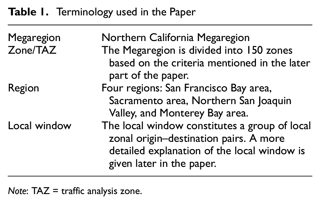
Note: TAZ = traffic analysis zone.

The organization of the paper is as follows. The next section covers the relevant literature on efforts to understand pandemic-related disruption/recovery of travel demand and various methods to compare OD matrices. The following section describes the study area and the data used in the study. We then provide a detailed discussion on how travel demand data were analyzed and the major patterns that were observed. The final section summarizes and concludes the paper.

Background and Use of Structural Similarity Index Measure

This section reviews the literature on two broad topics: (1) efforts to understand travel disruption and recovery during and after the pandemic and (2) methods to compare OD matrices.

Several researchers have studied the impact of the pandemic on travel patterns for different socioeconomic segments, in particular using data from travel surveys ( 13 – 17 ). As noted previously, surveys are often limited in their ability to provide information about continuously changing travel demand over the time periods of interest. In contrast, passively collected data from cell phones and other location-based services can address these dynamics and are becoming a popular option in the transportation research community for investigating a variety of research questions. However, they typically lack information on the sociodemographic and other characteristics (including lifestyles and attitudes) of the individuals who make the trips and the purposes for which the observed trips are made.

Many researchers have used passively collected or smart card data to understand changes in travel patterns during the pandemic ( 4 , 18 –25). For example, Bamney et al. used Streetlight data ( 20 ), and Dean and Zuniga-Garcia used raw Global Positioning System (GPS) data ( 24 ). However, there were some limitations in these studies. Most of them used aggregate metrics such as trip volume or VMT to quantify the impact of the pandemic. The pandemic has changed the way people travel, work, shop, study, and so forth, and it significantly affected travel activities. So, it is possible that, in some cases, the aggregate amount of travel, in relation to daily trip volume or VMT, has returned to pre-pandemic levels, but at a disaggregated level, travel demand has been changed heterogeneously, for example, by trip purpose, travel distance, temporal factors including time of day, day of the week, and spatial factors including land use, zonal properties, and sociodemographic including population characteristics and household income. There is, so far, evidence that this is indeed the case. For example, the decline and recovery of travel in the morning peak has been found to differ from the evening peak. Similarly, travel pattern changes also differ by trip purpose, as discussed in later sections.

We also provide a brief overview of methods for comparing OD matrices here. Trip volumes between different OD pairs can be correlated owing to similar properties, such as trip production/attraction and travel impedance ( 6 ). Similarly, trip volumes for the same OD pair measured at different times can exhibit temporal correlation ( 8 , 26 ). A more detailed discussion on spatial and temporal correlation can be found elsewhere ( 6 , 27 ). Traditional metrics associated with detailed analyses or regression models of OD travel data, such as mean squared error ( 28 ), mean absolute error ratio ( 29 ), Theil’s goodness of fit ( 30 ), R-squared ( 31 ), and entropy measures ( 32 ) typically fail to capture the spatial and temporal correlations between OD pairs.

Very few metrics have been proposed to address this limitation of traditional metrics. One such metric is the Structural Similarity Index Measure (SSIM), which is discussed in detail in the next subsection. The SSIM was originally proposed to compare two digital images ( 33 ) but has since been extended in several studies to compare travel demand with OD matrices ( 6 , 8 , 27 , 34 , 35 ). In digital images, the data matrix consists of measurements for individual pixels; however, pixel data from (meaningful) images necessarily have patterns that are spatially correlated. This type of structure can best be analyzed by grouping together adjacent pixels into sub-matrices. Using the same grouping definitions (sub-matrices) for data from two images, a similarity measure between corresponding pairs of sub-matrices can be computed. The traditional SSIMs for image analysis are typically computed using sub-matrices that are constructed via a “local sliding window” method, in which windows (sub-matrices of common size) slide cell by cell from the top-left to bottom-right. Two image matrices are compared using a summary measure over the individual SSIMs.

Each SSIM for a pair of sub-matrices is a product of three components. Two components (L and C) measure the similarity of the means and standard deviations of the two windows, respectively. The third component (STR) uses the correlation coefficient across the two windows. See Equations 1 to 3, where $x_{w}$ represents the window (sub-matrix) for the first image, and $\underset{w}{\hat{x}}$ is the corresponding window from the second image. The three components are combined using the expression in Equation 4, which includes three influence parameters.

L (x_{w}, {\hat{x}}_{w}) = \frac{(2 μ_{x_{w}} μ_{{\hat{x}}_{w}} + C_{1})}{(μ_{x_{w}}^{2} + μ_{{\hat{x}}_{w}}^{2} + C_{1})}

(1)

C (x_{w}, {\hat{x}}_{w}) = \frac{(2 σ_{x_{w}} σ_{{\hat{x}}_{w}} + C_{2})}{(σ_{x_{w}}^{2} + σ_{{\hat{x}}_{w}}^{2} + C_{2})}

(2)

STR (x_{w}, {\hat{x}}_{w}) = \frac{(σ_{x_{w} {\hat{x}}_{w}} + C_{3})}{(σ_{x_{w}} σ_{{\hat{x}}_{w}} + C_{3})}

(3)

\begin{matrix} SSIM (x_{w}, {\hat{x}}_{w}) = [L {(x_{w}, {\hat{x}}_{w})}^{α}] [C {(x_{w}, {\hat{x}}_{w})}^{β}] [STR {(x_{w}, {\hat{x}}_{w})}^{γ}]; \\ α > 0, β > 0, γ > 0; \end{matrix}

(4)

Assuming $α = β = γ = 1$ and $C_{3} = C_{2} / 2$ yields

\begin{matrix} SSIM (x_{w}, {\hat{x}}_{w}) = \frac{(2 μ_{x_{w}} μ_{{\hat{x}}_{w}} + C_{1}) (2 σ_{x_{w} {\hat{x}}_{w}} + C_{2})}{(μ_{x_{w}}^{2} + μ_{{\hat{x}}_{w}}^{2} + C_{1}) (σ_{x_{w}}^{2} + σ_{{\hat{x}}_{w}}^{2} + C_{2})} \\ [- 1 \leq SSIM (x_{w}, {\hat{x}}_{w}) \leq 1] \end{matrix}

(5)

For this study we use these same measures to compare pairs of OD matrices (i.e., not image matrices) at different points in time, where a key aspect of the methodology is specifying an appropriate procedure for defining sub-matrices for this type of data. Specifically, $x_{w}$ represents an OD sub-matrix for a week in 2019 and $\underset{w}{\hat{x}}$ represents a corresponding OD sub-matrix for the corresponding week between January 2020 and October 2021. $L (x_{w}, {\hat{x}}_{w})$ and $C (x_{w}, {\hat{x}}_{w})$ compare the mean values and standard deviations of the OD sub-matrices, respectively. $STR (x_{w}, {\hat{x}}_{w})$ computes the coefficient of correlation, and thus compares the structure of the sub-matrices. The coefficients $α$ , $β$ and $γ$ in Equation 4 are used to adjust the relative importance of each component and are generally set to 1. The constants $C_{1}$ , $C_{2}$ , and $C_{3}$ are included to provide mathematical stability and are set to small values. The values of $C_{1}$ and $C_{2}$ were set to $10^{- 10}$ and $10^{- 2}$ , respectively, and $C_{3}$ was set to $C_{2}$ /2 as mentioned in a previous study ( 34 ). Using these settings, the SSIM values lie between −1 and 1, where 1 represents perfect similarity, and −1 represents the maximum dissimilarity between the OD sub-matrices. An overall similarity measure between two OD matrices can be obtained by computing the mean SSIM (MSSIM).

Recall that, in the case of images, the way the data are stored ensures that neighboring pixels are generally spatially correlated. The analogous (purely spatial) concept for OD matrices would be zone adjacency. However, the way data are stored in OD matrices does not automatically take zone adjacency into account. Moreover, the factors that influence patterns of travel behavior between OD pairs are unlikely to be determined exclusively by spatial location. For example, zones with lower travel impedance (within a neighborhood) or zones with high levels of activity are not necessarily located “close” to each other geographically. In any case, the concept of “local sliding windows” originally developed to compare local “regions” of two image matrices is not relevant for comparing travel demand data represented in OD matrices.

Behara et al.’s methodology attempted to address this issue by proposing the concept of a geographical SSIM, in which the rows and columns of OD matrices are manually re-arranged based on geographic proximity, and “static local geographic windows” are defined for which OD pairs are grouped into predefined geographic “regions” ( 7 ). The SSIMs are computed for these regions and then aggregated to compute a GSSI (equivalent to MSSIM). However, the manual effort required for re-arranging zones and determining windows can be challenging to apply effectively to large OD matrices, limiting its practicality for capturing geography-based similarity in travel patterns. What is therefore needed to improve this approach is a practical way of selecting geographical regions or OD sub-matrices to calculate SSIMs.

This study improves the current methodology by proposing a new “local sliding geographical window” based on the natural flow of trips. The proposed “local sliding geographical window” slides over the study area (Megaregion) and is independent of the arrangement of zones in the OD matrix. More details are presented in the section on the analysis of travel patterns.

Study Area

This study focused on the Northern California Megaregion as the study area. Figure 1 shows the four regions: San Francisco Bay area, Sacramento area, Northern San Joaquin Valley, and Monterey Bay area. We divided the Megaregion into 150 Traffic Analysis Zones (a.k.a. “TAZs” or “zones”) for the purposes of this study, as shown in Figure 2. The three key considerations when defining the zone system are listed below:

Geographical and administrative boundaries

The 150 zones are formed by the aggregation of census tracts and are nested within county boundaries. This enables high-level analysis of intra- and inter-county travel patterns. Furthermore, local regulation and travel activity changes caused by the pandemic can be better studied with such a design.

Sociodemographic information

To the degree possible, census tracts were grouped to maximize the homogeneity of sociodemographic information such as income level and population density. In particular, certain zones are aggregations of disadvantaged communities derived from the MTC methodology ( 36 ) and SB535 criteria ( 37 ). This supports the analysis of activity and travel changes related to the needs of low-income areas and communities lacking proper access to mobility services.

Land use and infrastructure

The land use and infrastructure systems guide the shapes and sizes of the zones. “Place type” is the main attribute by which we cluster census tracts. Three place types were defined in a previous study ( 38 ): Urban (including Central City), Suburban (including Rural-in-Urban), and Rural. In addition, we specifically distinguish some local communities and urban centers. Examples include downtown San Francisco, downtown San Jose, and West Sacramento. These zones are especially helpful for studying telecommuting patterns. We also created dedicated zones for large university campuses, enabling the potential evaluation of remote teaching and COVID-19 impacts on densely populated areas, such as, Stanford University, the University of California, Berkeley, and the University of California, Davis. Major highway networks often serve as administrative and planning boundaries for local communities. Finally, we defined zones for major transportation hubs. Specifically, four zones are dedicated to major international airports, including the Sacramento International Airport, San Francisco Bay Oakland International Airport, the San Francisco International Airport, and the San Jose Mineta International Airport.

Figure 1.

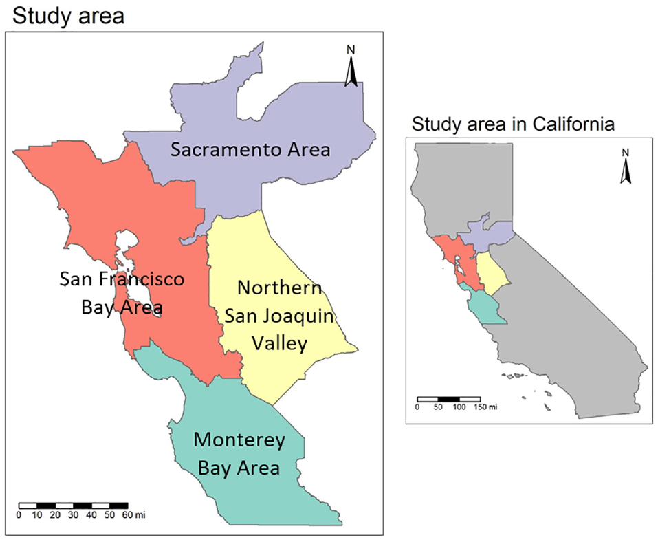
The left figure shows the study area. The right plot shows the study area on the map of California.

Figure 2.

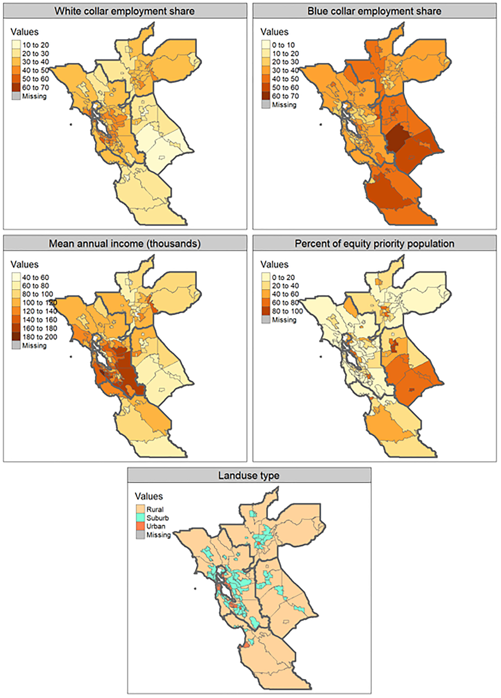
Sociodemographic and land-use characteristics of 150 zones in the study area. The wider line shows the boundaries of the four regions.

Beyond the abovementioned key considerations, we also acknowledge several constraints of the defined zone system. First, we were limited to a budget of 150 zones when purchasing the demand- and flow-related data from Streetlight Data. However, it is important to obtain enough data that can cover the Northern California Megaregion. This would also enable us to capture long-distance travel and their recovery from COVID. For example, trips between the Bay area and Sacramento region have been an important element of Northern California regional travel. As a result, each zone defined is much larger in spatial size than zones (TAZs) in the existing California Statewide Travel Demand Model. Second, from an estimation and computational perspective, finer resolution might not always lead to better efficiency and insights. A zoning system that is too detailed would add noise and computation burdens in studying characteristics for factors related to COVID-19. For example, smoothing operations are very common in spatial data analysis by aggregating the census tracts to a coarser granularity to allow us to denoise the data and capture the dominant structure in OD data over time.

Figure 2 highlights the variation in selected socioeconomic characteristics among the zones and regions. The San Francisco Bay area has the highest white-collar employment, higher mean income, and more urban and suburban land use, followed by the Sacramento area. The Northern San Joaquin Valley and the Monterey Bay are more rural and have a larger proportion of blue-collar jobs in the agriculture and industrial sectors. Some zones in the Northern San Joaquin Valley also have a large proportion of the equity-priority population. These variations among regions would lead to heterogeneous impacts of the pandemic on the regional travel demand.

Data and Period of Analysis

The passively collected, location-based data from the StreetLight Data platform ( 11 ) from January 2019 to October 2021 were used for analysis. This section gives a brief overview of the StreetLight Data, the study area, and the weekly OD matrices used in the analysis. StreetLight Data is a cloud database platform that receives GPS-trajectory data from various sources and uses them to compute datasets containing a variety of measures that are useful for transportation research applications, such as OD matrices. Several studies have used Streetlight data for various applications. MPOs and transit agencies have also been using Streetlight data, consistent with the findings of Yang et al. ( 39 ), who evaluated the StreetLight Data and provided recommendations on their use for planning applications. They advise using the data at varying levels of aggregation to reduce the estimation error, for example, over different time periods (days, weeks, months).

Weekly OD Matrices

We analyzed weekly OD matrices from January 2019 to October 2021. The OD matrices are segmented across six time periods of the day, three inferred trip purposes, and two types of days of the week. The six time periods are: all day, early AM, peak AM, midday, peak PM, and late PM. The early AM and peak AM correspond to the time between midnight and 6 a.m. and 6 a.m. and 10 a.m., respectively. The midday period corresponds to the time between 10 a.m. and 3 p.m. The peak PM and late PM refer to the time between 3 p.m. and 7 p.m. and 7 p.m. and midnight, respectively. The two types of days are weekdays and weekends. Weekdays included Monday to Thursday (but excluded Fridays), whereas weekends included Saturday and Sunday. In StreetLight Data’s default setting, Fridays are excluded from weekdays simply because they tend to deviate from more typical weekday traffic patterns (more people may be leaving work early, people tend to take Fridays off more frequently, etc.).

The StreetLight data infer home and work locations based on where devices spend their working hours and their night time hours. For example, work hours are defined as 11 a.m. to 4 p.m. on weekdays (M–F) ±1 or 2 hour, depending on the exact time zone and data month. But it also implies that if a given person is spending those work hours at an education institution, it may be considered as a work location. For more details on the methodology to infer home and work location, please see StreetLight Data ( 40 ). The home and work locations were used to infer the purpose of each trip and to assign it to one of three categories:

Home-based work trips: Trips for which one end is the inferred home location, and the other end is the inferred work location.

Home-based other trips: Trips for which one end is the inferred home location but the other end is not the inferred work location. For example, trips made from/to home to/from grocery stores.

Non-home-based trips: Trips for which none of the ends is the inferred home location. For example, trips made from workplace to grocery store.

Timeline of the COVID-19 Pandemic

The study period from January 2019 to October 2021 was divided into five stages of the pandemic, as defined by Wang et al. ( 25 ), based on the chronology of the pandemic and policy interventions in California. Each stage is described briefly.

Stage 0. Pre-COVID-19: 01/06/2019–03/09/2020. This period served as the baseline for pre-pandemic average daily trip volume.

Stage 1. COVID-19 outbreak: 03/10/2020–08/30/2020. This period experienced strict policies, such as stay-at-home orders, to contain the spread of the COVID-19 virus.

Stage 2. Start of the Blueprint: 08/31/2020–12/31/2020. This period represents the time between the launch of the Blueprint framework and the start of vaccination. The stringency varied across county and time.

Stage 3. Start of Vaccination: 01/01/2021–06/14/2021. This period is between the start of vaccination and the full reopening of the State of California.

Stage 4. Fully Reopen: 06/15/2021–10/24/2021. This period is after the lifting of all statewide restrictions (retirement of the Blueprint) until the end of the study period. This period marks the lifting of state interventions but the continuation of private sector policies, for example, allowing remote working.

Analysis of Travel Patterns

The study attempts to explore the extent of variability in the impact of the pandemic on travel demand through three main components.

Temporal Variation in Trip Volume: This initial phase of our analysis involves an exploratory examination aimed at quantifying the impact of the pandemic on trip volume within the Megaregion. We also investigated the heterogeneity in the impact across time of the day, day of the week, and trip purpose. The result from this exploratory analysis should help us to see any variation in trip volume and suggest what types of travel patterns should be investigated further.

Spatial–Temporal Variation of Travel Demand within Individual Regions: This is the second phase of analysis, delving into comprehensive examinations of spatial–temporal patterns through the utilization of OD matrices for individual regions. In this study, there are four regions, namely, the San Francisco Bay area, the Sacramento area, the Northern San Joaquin Valley, and the Monterey Bay area. Here, we use the concept of structural similarity to compare travel patterns inferred from OD matrices. This is achieved by using an existing metric, SSIM, as discussed in the literature review section. Although the analysis in this section surpasses the sole reliance on trip volumes, as seen in the initial part, by capturing the two-dimensional nature of travel through OD matrices, it is important to note that the examination of each region is conducted independently. This approach does not account for the natural flow of trips between the regions. The subsequent section of the analysis delves deeper into addressing this limitation.

Spatial–Temporal Variation of Travel Demand at a local level: The third part involves the analysis at a more refined level to study the extent of variability in the impact of the pandemic at local regions. This is accomplished by refining the application of SSIM, transforming the traditional “sliding window” into a “local sliding geographical window.” A “local sliding geographical window” for a specific zone encompasses all OD pairs that account for 90% of trips originating from that zone. This approach ensures that trips originating from and ending in any of the four regions (San Francisco Bay area, Sacramento area, the Northern San Joaquin Valley, and Monterey Bay area) falling within the 90% threshold are included, enabling the capture of the natural flow of trips across these regions. If there are 150 local zones, we have 150 local sliding geographical windows corresponding to those zones. Additionally, we independently examine the temporal changes in the weekly OD matrices using SSIMs for each local sliding geographical window (group of local zonal pairs). These temporal variations across diverse local sliding geographical windows reflect spatial variation or spatial heterogeneity.

The following sub-sections first discuss the temporal variation in trip volume in the Northern California Megaregion and then discuss more detailed spatial–temporal variations at the regional and local levels. The key findings are presented together later in this section.

Temporal Variation in Trip Volume

The temporal variation in absolute daily trip volume and relative trip volumes were analyzed by time of day, day of the week, and trip purpose, as shown in Figures 3 and 4. The relative daily trip volumes from January 2020 to October 2021 are estimated with respect to the average daily trip volume of the corresponding weeks in 2019. A three-point moving average was employed to smoothen the temporal variation in trip volumes because some weeks in the study period may contain holidays, long weekends, or other special events. This preliminary analysis quantified the decline and recovery trends of trip volumes across the study period. It also highlights that the decline and recovery of trip volumes varied by time of the day, day of the week, and trip purpose. The impact on trip volume during different stages of the pandemic is discussed briefly.

Stage 0 – pre-COVID: In the second week of January 2019, an estimated 30.3 million average daily trips were made on weekdays within the Megaregion. The daily volume remained similar until the first week of March 2020, apart from some usual seasonal variations.

Stage 1 – COVID Outbreak: The trip volume dropped significantly after the stay-at-home orders were enforced to contain the spread of the COVID-19 pandemic. The average weekday trip volumes dropped by nearly 47% by the first week of April 2020 compared with the first week of April 2019. The decline in the daily trip volume varied by trip purpose, time of day, and day of the week. The average daily home-based work trips dropped by 37%, daily home-based other trips by 46%, and daily non-home-based trips by 56% on weekdays during the first week of April 2020 with respect to the first week of April 2019. Figure 4 suggests a relative recovery of peak AM home-based work trips during June–August 2020 when compared with the same period in 2019. However, further investigation, including discussions with StreetLight Data, revealed that this apparent increase could partially be attributed to a decrease in the home-based work trips during June–August 2019. A potential explanation for these decreases is school and college vacations, which reduce the number of trips between home and educational institutions that are considered work trips in the StreetLight data. Further work and cross-checking with additional data sources and models are essential to either understand the underlying causes or to validate the StreetLight data.

Stage 2 – Blueprint and Stage 3 – Vaccination: The trip volume remained stable and slightly recovered during these stages. The recovery of non-home-based trips was the slowest among the three trip purposes. However, the recovery of home-based work trips was the slowest during peak AM. People with more flexibility in work likely continued to work remotely, at least partially, during this period.

Stage 4 – Fully Reopen: When the statewide restrictions were lifted, the home-based work trip during peak AM largely rebounded from 29% below the base level in June 2021 to 10% below the base level in October 2021. Notably, the average weekday trip volumes had also recovered to the pre-pandemic level by October 2021 and were 8% below the corresponding week in 2019.

Overall, the non-home-based trips experienced the largest disruption and lagged in their recovery. Non-home-based trips represent those that neither start nor end at home, for example, trips made from the workplace to a grocery store or from a restaurant to a friend’s place. There are multiple possible reasons for these changes. First, we interpret this finding as the fact that travel tours became simpler during the pandemic. For example, during the pandemic, people traveled to work or to carry out other activities and returned home, avoiding making stops at grocery stores, coffee shops, gyms, and so forth for other activities. Others switched to remote work and reduced the number of commuting trips, and from their home location, they traveled to a third location and then directly back home. The persistence of forms of hybrid remote work is also responsible for the slower recovery in this type of trip, as there are fewer occasions to originate a trip from a non-home location such as work.

Figure 3.

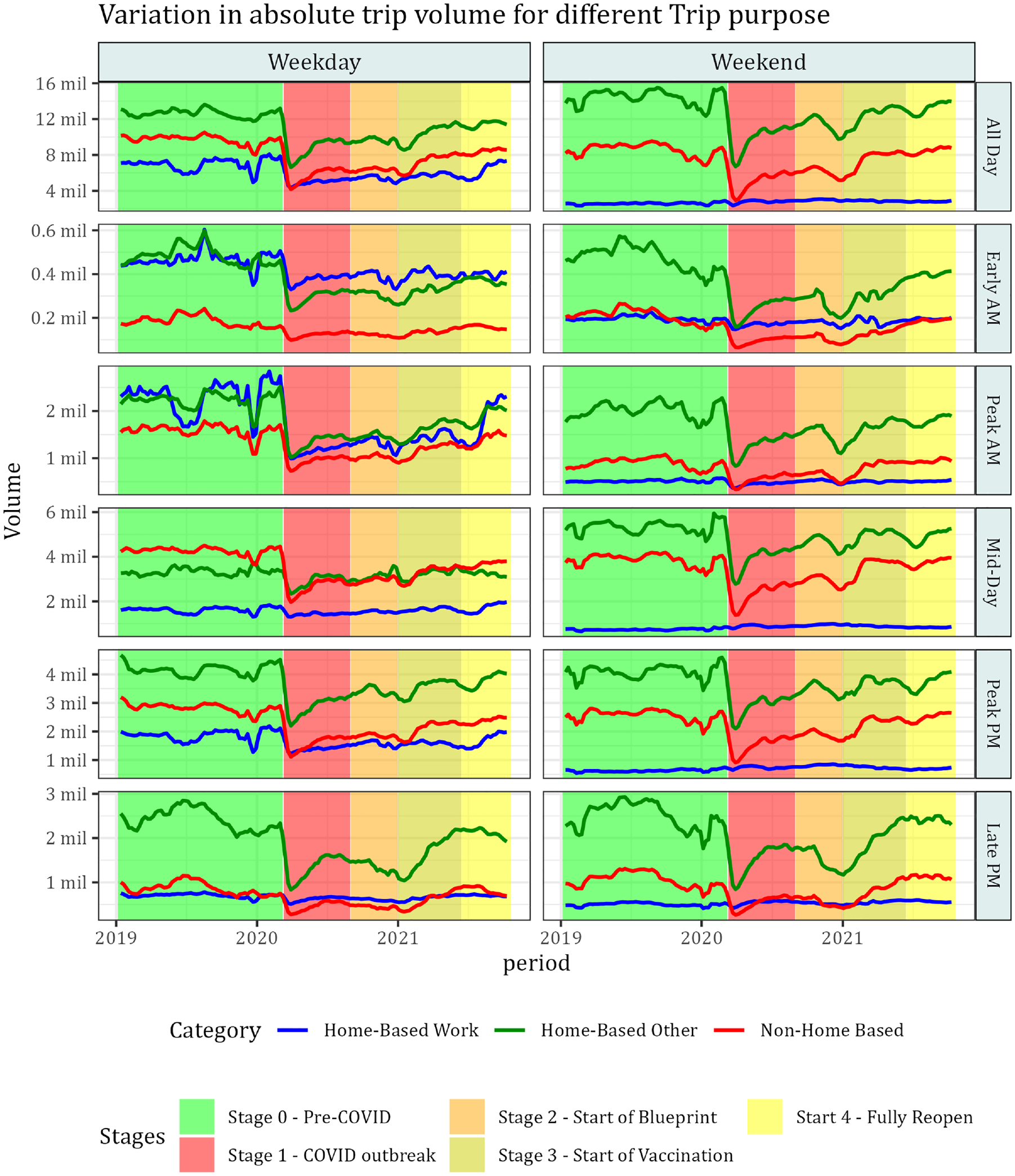
Variation in estimated average daily trip volumes (in million) by trip purpose from January 2019 to October 2021.

Figure 4.

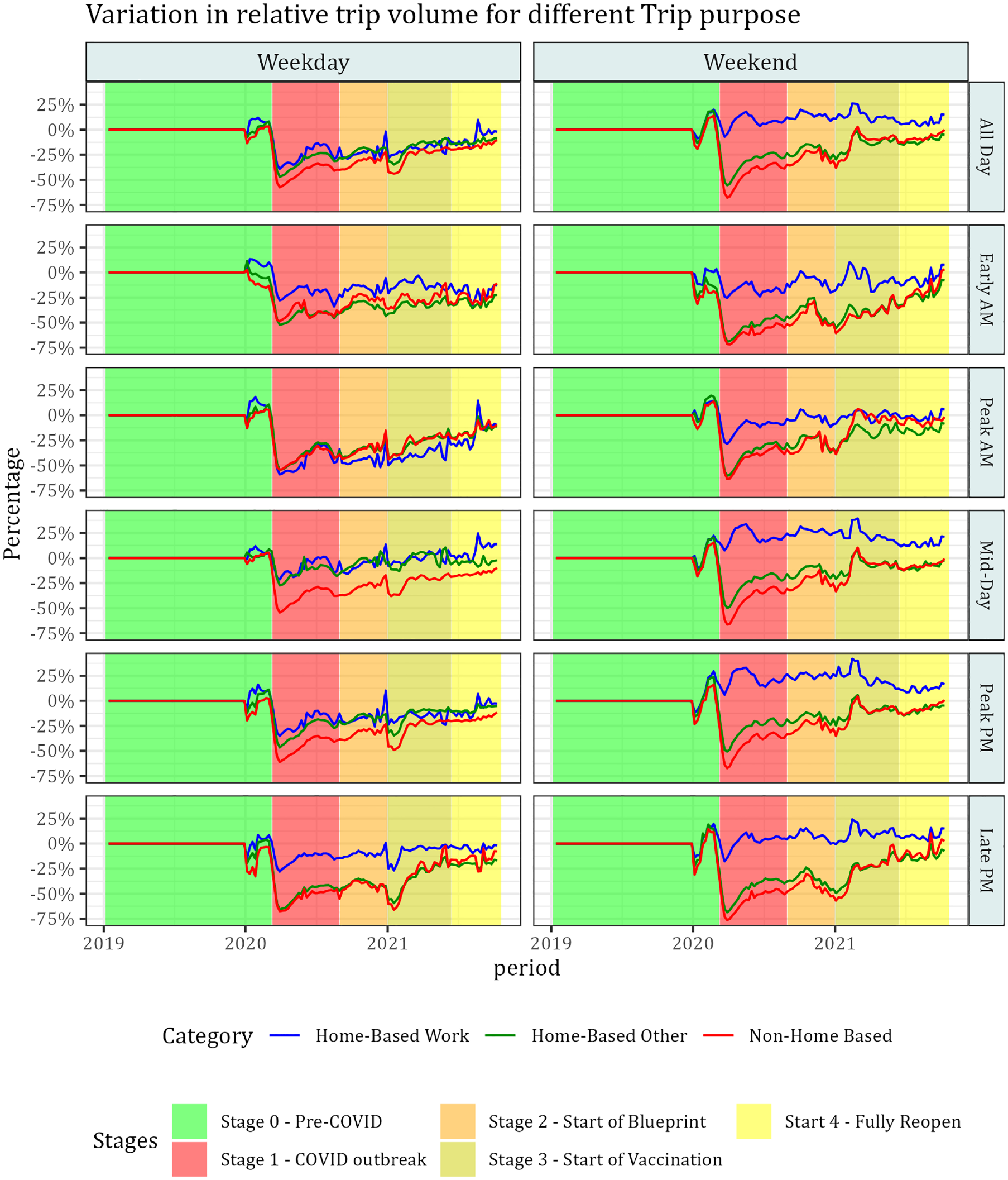
Variation in relative average daily trip volumes by trip purpose from January 2020 to October 2021 with respect to volume in corresponding weeks in 2019.

Spatial–Temporal Variation of Travel Demand within Individual Regions

The temporal variation in trip volume can provide some preliminary information about the trends. However, the aggregate measure (trip volume) fails to capture the underlying spatial variations. For example, the non-home-based trips for a local region (during late PM on weekends) in June 2021 were 43% below the trips in the corresponding week in 2019, also as the result of the fewer people that were at work and could start trips from the work location in the afternoon.

The heatmap in Figure 5 highlights an example of the variation in relative recovery in trips among OD pairs. The red color represents those OD pairs where trip volumes were significantly below the pre-pandemic level (corresponding week in 2019), and the yellow color represents those OD pairs that nearly recovered. The green color represents those OD pairs where trips in 2021 were higher than the pre-pandemic level. It is also important to note that the heatmap in the figure represents a relative change (not an absolute change), and the OD pairs with green color had smaller absolute trip volumes. However, the figure clearly illustrates the spatial variation in the decline and recovery of trip volume in a region, and therefore, it emphasizes the importance of comparing the OD matrices (a disaggregate measure) across time to study the impact of the pandemic. In the later sections, we compare OD matrices across time using a technique called SSIM.

Figure 5.

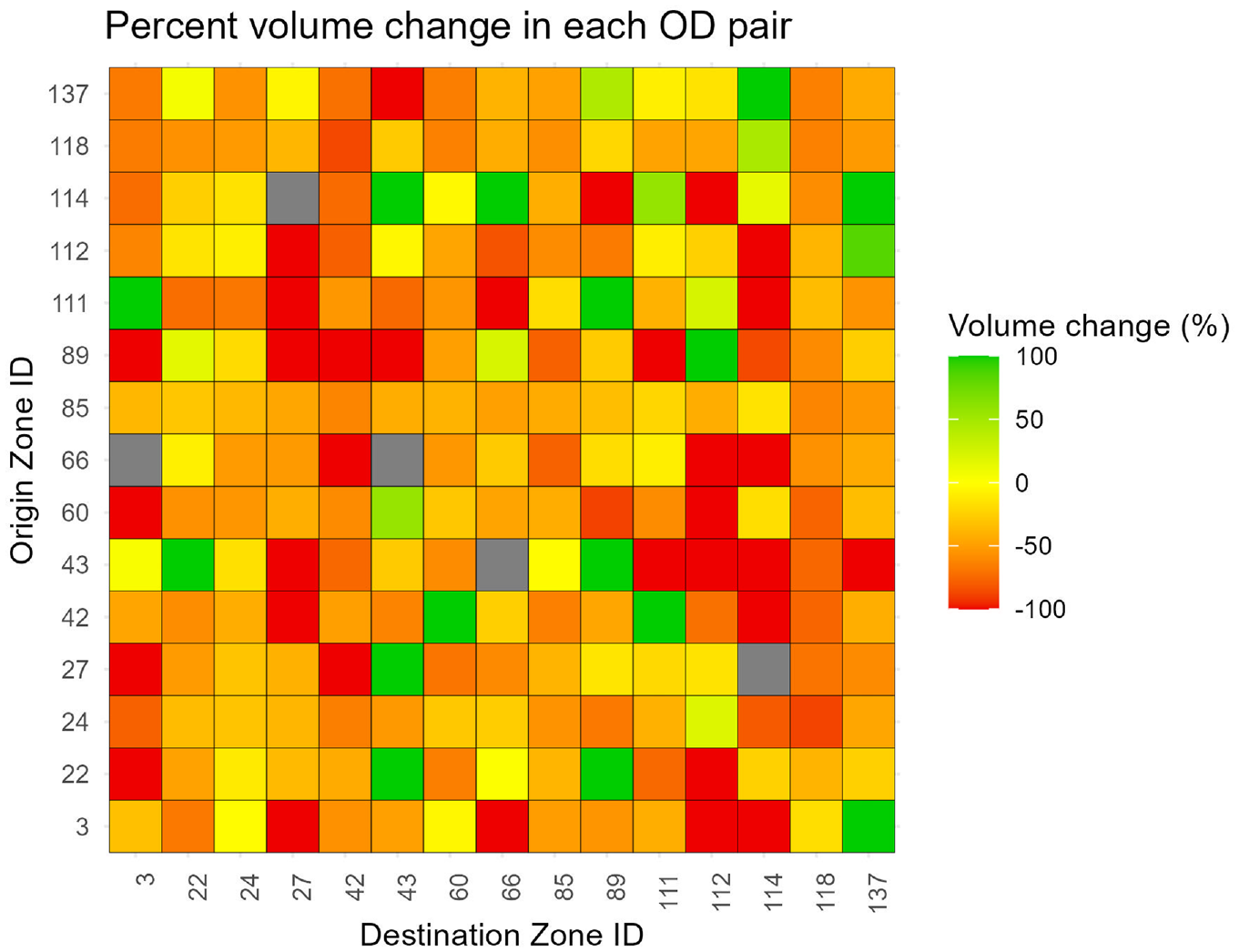
Example of variation in trip volume change across origin–destination pairs in a region.

The preliminary analysis of trip volumes establishes the basis for a comprehensive and in-depth spatial–temporal analysis. It is crucial for MPOs, policymakers, traffic management centers, and transportation planners to understand variations in travel demand during the pandemic and recovery phases. This knowledge supports the targeted and optimal allocation of limited resources, such as financial investments and mobility funds, to meet the public’s needs effectively. In addition to trip generation, knowing the destinations of these trips is vital for informed decisions about transportation planning and policy. It is well known that OD demand matrices have always played a key role in the travel demand modeling process, enabling the prioritization of OD pairs for transportation (including transit) improvement and the identification of congested corridors during peak periods. The next portion of this section presents results from a detailed spatial and temporal analysis building on insights from the preliminary examination of trip volumes and OD matrices. By comprehensively studying local spatiotemporal patterns, this analysis will inform effective strategies for addressing travel demand fluctuations, optimizing transportation services, and ensuring a resilient and sustainable transportation network in the face of future challenges.

To investigate the spatial–temporal pattern in travel demand, we computed weekly SSIM values of each region from January 2020 to October 2021 by comparing them with the corresponding weeks in 2019 to account for seasonal variations. Similar to the previous analysis, a three-point moving average was employed to smoothen the SSIM curves because some weeks in the study period may contain holidays, long weekends, and other special events, which could affect the OD demand. The resulting time series curve of SSIMs for each region captures the temporal variations in travel demand, and the variations between these curves across regions can reveal spatial heterogeneity in the disruption and recovery of travel. Note that the SSIM values lie between −1 and 1, where 1 represents occurs when an OD matrix is perfectly similar to its counterpart in 2019, and −1 occurs when an OD matrix is maximally dissimilar to its 2019 counterpart. Because this methodology is totally new, there are no benchmarks from existing literature for comparison purposes. Moreover, these specific results are a function of the parameters used in the SSIM definitions, as well as the approach to defining regions. Our ability to provide heuristics on the relative meaning of these similarity measures will continue to develop as follow-up phases of this work are carried out in the future.

Figure 6 highlights the variation in disruption and recovery of travel demand (OD patterns) of home-based work trips during peak AM among the four regions of the Northern California Megaregion.

Stage 0 – pre-COVID: The travel demand in the early months of 2020 was similar to 2019. However, in the early weeks of March, the work commute started to decline rapidly. The decline in travel demand was sharpest in the San Francisco Bay area, followed by the Sacramento area. Both regions have a higher proportion of white-collar workers (as shown in Figure 2), compared with the other regions in the study—this allowed more residents in the San Francisco Bay area and in the Sacramento area to work from home even before the stay-at-home orders were implemented. This would not be surprising, considering the awareness among and strong international ties of the California high-tech industry with international contexts, and in particular, the relationships with China, where the pandemic spread earlier on than in the United States.

Stage 1 – COVID Outbreak: During the early phase of the outbreak, all regions experienced significant changes in their OD patterns. Again, the San Francisco Bay area experienced maximum disruption in the OD patterns. The disruptions were similar for the Sacramento area, which also has a significant number of government jobs and rapidly growing hi-tech employment. The figure shows some relative recovery in the OD patterns during June–August 2020. However, as we discussed earlier, we believe that this relative recovery partially appears because of a drop in peak AM home-based work trips in June–August 2019, which is likely caused by school and college vacations. We observed similar recoveries in November 2020 owing to Thanksgiving holidays and December 2020 to Christmas holidays.

Stage 2 – Blueprint and Stage 3 – Vaccination: During these stages, the OD patterns of all the regions gradually and steadily recovered. However, the SSIM curves during these stages clearly highlight the significant regional variations in the recovery. The recovery in the San Francisco Bay area was significantly below that of the other three regions. However, demand started to recover quickly after April 2021. There are a few possible reasons for the rapid recovery, such as the vaccination of a large proportion of the residents, the reopening of some offices, and the reduced COVID-related restrictions. In Stage 3, the recovery of Sacramento and Northern San Joaquin Valley followed each other very closely. Travel demand in the Northern San Joaquin Valley recovered fastest among all four regions and returned to the pre-COVID level by the end of Stage 3. The SSIM curves at the end of December 2020 give an impression of a sharp recovery of travel demand. However, it is important to note that the end of December is a holiday season, and therefore the comparison of travel demand refers to a season in which commuting flows remained low(er), as well as in December 2019. The OD patterns from 2019 and 2020 looked similar in December, which led to recording the relatively abrupt jump (recovery) in the SSIM values.

Stage 4 – Fully Reopen: The OD patterns of the Sacramento area and Monterey Bay area had nearly returned to the pre-COVID levels by August 2021. However, the OD patterns in the San Francisco Bay area were still different from the corresponding weeks of 2021, and they continued to recover until October 2021. The decline or recovery of travel patterns appears to be closely associated with socioeconomic and land-use patterns such as mean income and type of employment. The San Francisco Bay area, which has a higher mean income and a high proportion of white-collar workers, experienced maximum disruption and late recovery compared with other regions. The Northern San Joaquin Valley, which has a higher proportion of blue-collar workers associated with the industrial and agricultural sector and a large equity-priority population, experienced the least disruption and quickest recovery. The other two regions experienced intermittent impact.

Figure 6.

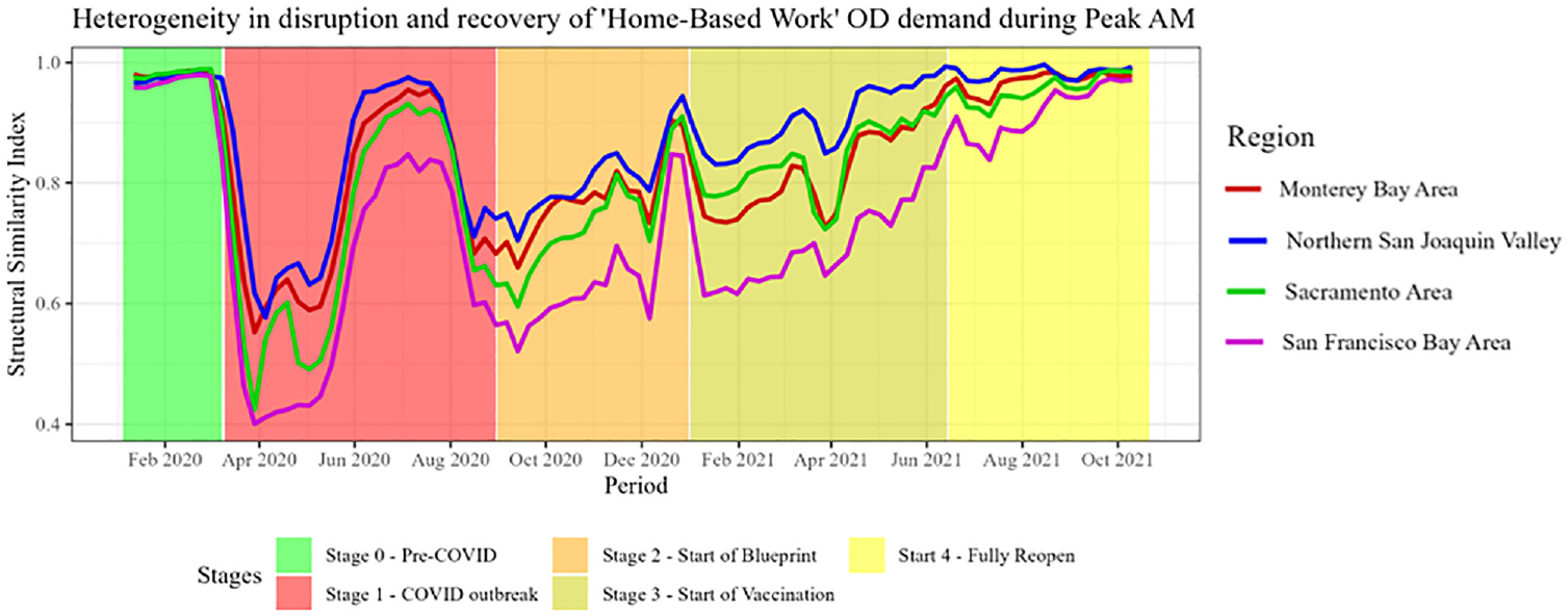
Illustration of heterogeneity in disruption and recovery of demand of home-based work trips during peak AM.

Spatial–Temporal Variation of Travel Demand at Local Level via Local Sliding Geographical Window

Although the result in the previous section establishes heterogeneity among four regions, it is important to note that there are 160+ cities in the Megaregion, which are managed by several transportation planning organizations, local and regional transit agencies, and traffic management centers. It is also important to investigate the extent of variability among local regions to support the local agencies in decision-making and optimally allocate resources among them in case of future pandemics.

Unlike the previous analysis, we do not predefine local regions here for two reasons. First, in this study, we were limited to defining only 150 local zones, some of which are as large as counties. Second, there are large numbers of trips that are made across administrative boundaries (cities and counties) for many reasons, including:

High rent values force people to live in more affordable locations and, from there, commute to work. For example, the growth in the Northern San Joaquin Valley commuters to the Bay area has been particularly dramatic, more than doubling from 1990 to 2013 and now comprising 15.8% of the Northern San Joaquin Valley’s resident workforce ( 10 )

There is increased emphasis on cross-county development, which induces more trips across administrative boundaries (cities, counties, regions).

For these reasons (among other reasons explained in the section), it is important not to predefine the regions but to have a more flexible definition. For each zone in the study area, we defined a local sliding geographical window (or region of influence of the zone) as the set of top destination zones where up to a threshold of 90% of the daily trips terminate. This proposed definition of the local window in the study area has the following benefits over the existing windows in the literature:

The defined window (group of local zonal OD pairs) is independent of the position of zones in the OD matrices and overcomes the issue of zone adjacency ( 8 , 27 ). The region corresponding to a zone remains the same regardless of the arrangement of zones in the OD matrix.

The proposed definition does not require manual re-arrangement of zones in the case of GSSI ( 7 ) or calculation of Euclidean distances as in the case of 4D-SSIM ( 35 ), which could be time-consuming and computationally expensive, respectively. The Euclidean distance is automatically accounted for.

The proposed definition allows the regions to be discontinuous. It can include distant zones if they fall under the defined criteria of the top destination zones. Please see Figure 7 for an illustration.

Figure 7.

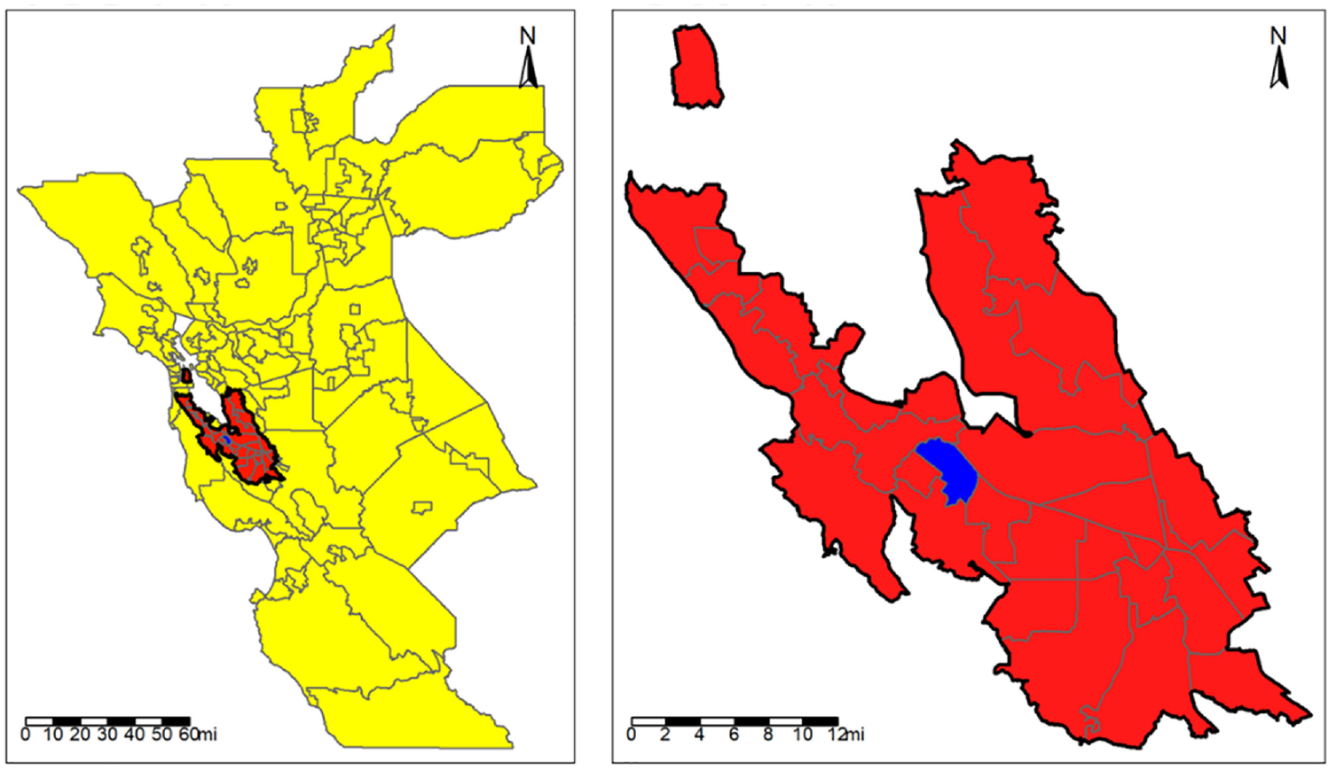
The left plot shows one of the local windows (in red) in the study area (in yellow). The right plot shows the zoomed plot of the same window; the zone colored in blue is used to create the window.

We created 150 local sliding geographical windows corresponding to each zone in the study area. The left plot in Figure 7 shows an example of one of the regions in the study area, and the right plot shows the zoomed-in image for the same region. The red-colored zones are the top zones where up to 90% of the trips generated from the blue-colored zone terminated (i.e., the red zones are the destination zones for trips that are generated in the blue origin zone). The algorithm calculates a regional SSIM for each local window in iteration. It can be visualized as a “local geographical window” sliding through the study area and computing the SSIM for each geographical window.

Moreover, we analyzed the OD matrices for different trip purposes and periods of the day to gain insights into the spatial–temporal patterns of travel demand. We repeated the process in five different time periods for three different trip purposes, weekdays and weekends. We used parallel programming in R language to accelerate this computationally intense exercise and compared over half a million local OD matrices in this portion of the study.

Figures 8 to 10 provide the spatial–temporal variation in the similarity indexes for home-based work, home-based other, and non-home-based trips. Results from all 150 zones are compiled using ribbon plots to show the variation for all SSIM curves during the study period. The width of the lighter ribbon plot provides the range of SSIMs across all regions at a given time period and represents the overall spatial heterogeneity in disruption or recovery of OD demand. The darker ribbon plot in the center represents the interquartile range of the regional SSIM values. The darker ribbon plots were superimposed on the lighter ribbon plots, which provided an indication of the distribution of SSIMs at any given time. If the darker ribbon is centrally placed, it indicates that SSIMs for a given week are symmetrically distributed. However, if the darker ribbon is not centrally placed on the lighter ribbon, it indicates a skewed distribution of SSIMs. In each figure, the left panel is for weekdays, and the right panel is for weekends. The top panel provides the SSIM ribbon for the whole day, whereas the other panels provide SSIM ribbons for different time periods of the day.

Figure 8.

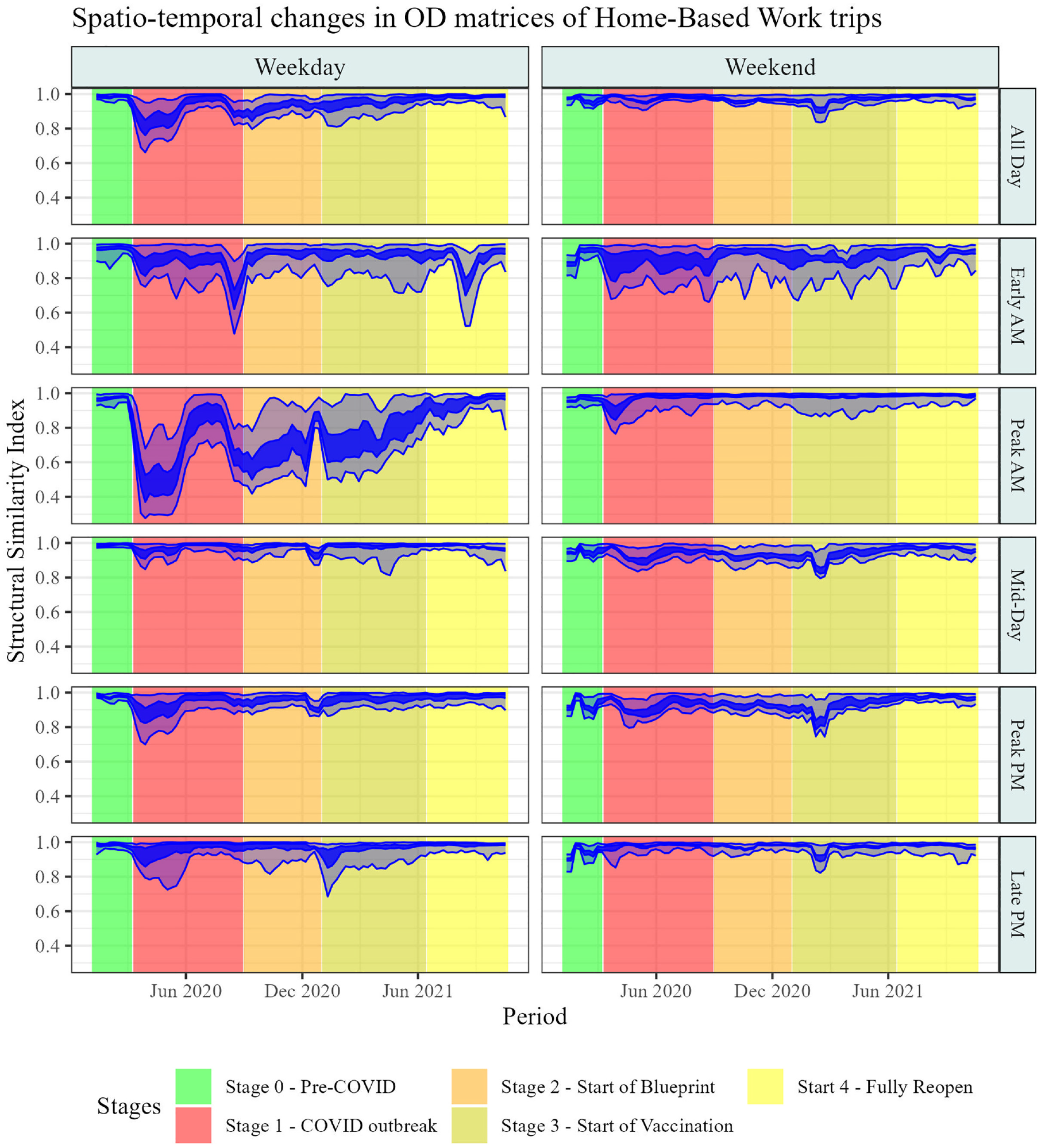
The spatial and temporal variation of Structural Similarity Index Measure values of weekly origin–destination matrices of home-based work trips with respect to the corresponding week in 2019.

Figure 9.

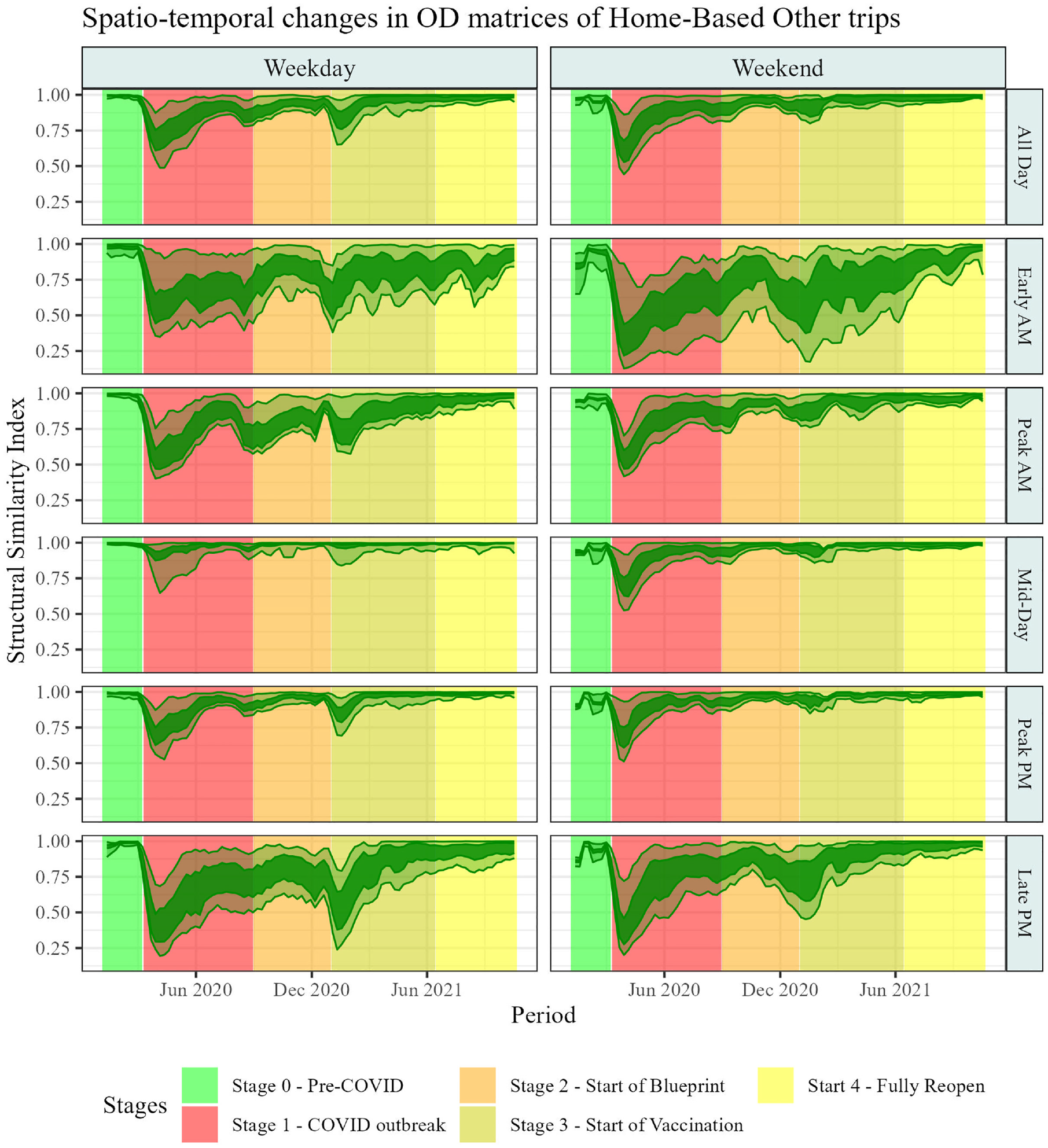
The spatial and temporal variation of Structural Similarity Index Measure values of weekly origin–destination matrices of home-based other trips with respect to the corresponding week in 2019.

Figure 10.

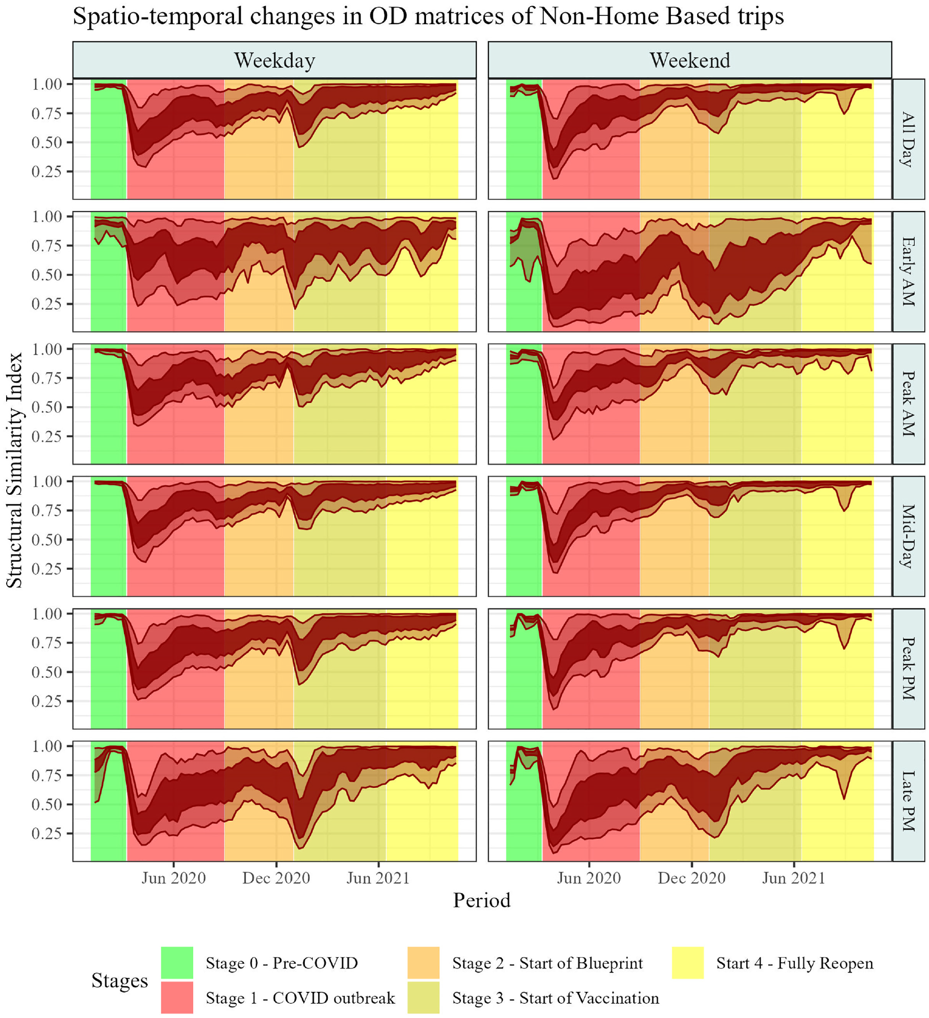
The spatial and temporal variation of Structural Similarity Index Measure values of weekly origin–destination matrices of non-home-based trips with respect to the corresponding week in 2019.

Figures 8 to 10 clearly demonstrate the heterogeneous impacts of the pandemic on travel demand. OD demand witnessed the largest disruption and significant regional variation for home-based work trips during the AM peak time (6 a.m. to 10 a.m.) on weekdays. The peak AM period accounted for an average of 2.3 million daily home-based work trips in the second week of January 2019. The OD demand for home-based work trips experienced the largest total disruption during the pandemic. The results also demonstrate significant regional variations in the disruption and recovery patterns of the OD demand. Some regions, such as the Bay area, with a high proportion of white-collar jobs, experienced significant changes in the OD demand in the early stages of the pandemic and slow recovery as more residents had the option to work from home. Other rural regions, with a larger proportion of blue-collar jobs, experienced smaller disruptions and faster recovery of OD demand, as more residents had to continue to travel for work during the analyzed period. After the initial disruption, Figure 8 highlights that the travel demand recovered in June–August 2020, which is mainly because of the decline in trips in June–August 2019, as discussed before. However, the travel demands experienced disruption again for the next few months, possibly because of subsequent waves of the pandemic.

OD demand witnessed a large disruption and significant regional variation in the disruption and recovery patterns of home-based other trips from late PM to early AM (7 p.m. to 6 a.m.), as shown in Figure 9. Home-based other trips represent trips that either start or end at home, but the other end is not a workplace, for example, a trip from home to the grocery store. The late PM and early AM periods account for 11 hours, but only 20% of home-based other trips in the second week of January 2019. Some reasons for the significant disruption during the pandemic include the “stay-at-home” orders, closed businesses, and fear of getting the infection. However, the analysis demonstrated significant variations in the regional disruption and recovery of the OD demand during this period.

The differences in the ribbon plots in Figures 8 to 10 demonstrate the heterogeneity in disruption and recovery of travel demand by region, time of the day, day of the week, and trip purpose. The SSIM values may not be directly interpretable, but they still provide a means for relative comparisons between different time points. Even though the absolute values are difficult to comprehend, the trends provide meaningful insights and are helpful in digging into underlying dynamics.

For further investigation, similar plots were developed for different components of SSIM (as mentioned in Equations 1–3) but not presented in the paper. The plots of STR, which represent structural similarities among OD matrices, have shown show that the STR values remained close to 1 in most of the plots. It indicates that the OD demand changed, but the structure of OD matrices remained relatively similar during the study period.

Summary and Conclusion

Many studies have examined the shifts in travel patterns resulting from the pandemic and the ongoing evolution of travel demand in the post-pandemic era. Measures such as trip volumes help explain the temporal variations in the impact of the pandemic on travel demand. However, along with trip volume, an OD-level analysis by time of day and day of the week helps us better understand spatial–temporal patterns at the local/regional level during and after the pandemic.

The objective of this work is to study the temporal patterns in trip volumes and develop a data-driven method to analyze the spatial–temporal patterns in the disruption and recovery of travel demand during and after the COVID-19 pandemic by analyzing OD matrices for different regions, time of day, day of the week (weekday and weekend), and trip purpose. This study used passively collected, location-based data from the StreetLight Data platform in the form of weekly OD matrices of all vehicle modes between January 2019 and October 2021. The study period was divided into five stages of the pandemic (Stage 0 to Stage 4). We studied the Northern California Megaregion, which has four regions: San Francisco Bay area, Sacramento Area, Northern San Joaquin Valley, and Monterey Bay area. The Megaregion was subdivided into 150 zones.

The study explores pandemic-induced variability in travel demand through three phases:

Temporal variation in trip volume: This is to quantify the pandemic impact on the Megaregion trip volume, examining temporal variations for further pattern analysis.

Spatial–temporal variation within regions: This is to utilize OD matrices and SSIM for an in-depth analysis of four regions, moving beyond trip volumes while considering regional independence.

Spatial–temporal variation at the local level: This part of the analysis redefined SSIM with a “local sliding geographical window,” capturing 90% of trips for each of the 150 zones. This reveals temporal changes, reflecting spatial heterogeneity across the Megaregion.

One of the paper’s key contributions lies in advancing the technique used to compute SSIM for OD matrices through the proposed local sliding geographical window. This innovative approach enhances the accuracy and reliability of comparing OD matrices, bringing a valuable improvement to the field. The advantages of this proposed definition are: (1) the regions are independent of the position of zones in the OD matrices and overcome the issue of zone adjacency, (2) the OD matrices do not require to be re-arranged, and (3) it allows the regions to be very flexible and discontinuous. We created 150 local regions corresponding to each zone in the study area and later calculated local SSIMs each week during the study period.

This study analyzed temporal patterns of trip volumes and spatial–temporal patterns in regional travel demand during and after the pandemic using weekly OD matrices. It provides empirical evidence of heterogeneity in the disruption and recovery of travel demand by region, time of the day, day of the week, and trip purpose. Some key insights into temporal patterns are as follows:

By the first week of April 2020, average weekday trip volumes had decreased by almost 47% compared with the same period in April 2019.

Home-based work trips dropped by 37%, home-based other trips by 46%, and non-home-based trips by 56% on weekdays during the first week of April 2020 with respect to the first week of April 2019.

By October 2021, daily trip volumes on weekdays had nearly recovered, with only an 8% difference compared with October 2019.

Non-home-based trips experienced the most significant disruption and slower recovery owing to changes in travel patterns and continued remote work.

Key findings from the spatial–temporal analysis for individual regions include:

The initial months of 2020 mirrored the travel demand patterns from 2019, followed by a sharp decline in work commute trips, in particular, in March. The San Francisco Bay area and Sacramento Area, with more white-collar workers, experienced the steepest declines.

All regions experienced significant OD pattern changes. The San Francisco Bay faced the largest disruptions, followed by Sacramento. Recovery in May–July 2020 might be data-related, an issue that is sometimes associated with the use of passively collected data and data-driven approaches.

Gradual recovery with notable regional variations was observed, with travel flows in San Francisco lagging but then improving after April 2021. Trips in the Northern San Joaquin Valley recovered fastest, returning to pre-COVID levels before the other regions.

Sacramento and Monterey Bay returned to pre-COVID levels by August 2021, whereas San Francisco took several more months to experience a similar recovery.

Disruption and recovery are likely linked to socioeconomic factors. San Francisco, with higher income and high-tech and government white-collar jobs, faced maximum disruption. Northern San Joaquin Valley, with blue-collar workers, experienced the least disruption and quickest recovery. Other regions had intermittent impacts.

More insights were found using local SSIM plots (considering the natural flow of trips across the regions) for different trip purposes. The OD structure was found to be less affected by the pandemic, suggesting that the structure of travel patterns did not change much during the pandemic. However, the changes in SSIMs were mainly contributed to by the varying trip volumes:

The largest disruptions occurred in home-based work trips during weekday mornings and home-based other trips during late evenings and early mornings.

The regions with more white-collar jobs had slower recoveries for work trips, whereas rural areas with blue-collar jobs recovered faster.

Late PM to early AM home-based other trips faced significant disruption because of “stay-at-home” orders, business closures, and infection fears.

Significant regional variations were observed in the disruption and recovery of home-based trips during the pandemic.

The analysis of the pandemic’s heterogeneous impacts helps policymakers at the local/regional level identify the modified spatial/temporal travel demand patterns and help allocate the limited resources—for example, for transportation investments and public transit funding—better. It can also contribute to designing future guidelines for pandemic preparation by better understanding the sensitivity of certain types of trips on various corridors with a modification of commuting versus other components of travel demand. Further, the work can be extended to learn the factors responsible for heterogeneity in disruption and recovery. Future extensions will consider regressing regional SSIMs representing the heterogeneity in recovery against aggregate sociodemographic and land-use characteristics such as mean household income and share of various employment types to explain the reasons behind the observed patterns.

Footnotes

Author Contributions

The authors confirm contribution to the paper as follows: study conception and design: Siddhartha Gulhare, Ran Sun, Keita Makino, Giovanni Circella; data collection: Giovanni Circella, Ran Sun, Siddhartha Gulhare; analysis and interpretation of results: Siddhartha Gulhare, Ran Sun, Keita Makino, Giovanni Circella, Krishna Behara, David Bunch; draft manuscript preparation: Siddhartha Gulhare, Ran Sun, Keita Makino, Krishna Behara, Daivd Bunch, Giovanni Circella. All authors reviewed the results and approved the final version of the manuscript.

Declaration of Conflicting Interests

The author(s) declared no potential conflicts of interest with respect to the research, authorship, and/or publication of this article.

Funding

The author(s) disclosed receipt of the following financial support for the research, authorship, and/or publication of this article: This study was made possible with funding received by the University of California Institute of Transportation Studies from the State of California through the Road Repair and Accountability Act of 2017 (Senate Bill 1). Additional funding was provided by the 3 Revolutions Future Mobility (3RFM) program of the University of California, Davis.

ORCID iDs

Siddhartha Gulhare

Ran Sun

Keita Makino

Krishna Behara

David S. Bunch

Giovanni Circella

References

King

Amberg

Wasserman

J. L.

Taylor

B. D.

Wachs

LOST and Found: The Fall and Rise of Local Option Sales Taxes for Transportation in California Amidst the Pandemic. In Pandemic in the Metropolis ( Loukaitou-Sideris

Bayen

A. M.

Circella

Jayakrishnan

, eds.), Springer International Publishing, Cham, pp. 63–78.

Speroni

Taylor

B. D.

Hwang

Y. H.

Pandemic Transit: A National Look at the Shock, Adaptation, and Prospects for Recovery. In Pandemic in the Metropolis ( Loukaitou-Sideris

Bayen

A. M.

Circella

Jayakrishnan

, eds.), Springer International Publishing, Cham, pp. 267–281.

Loukaitou-Sideris

Bayen

A. M.

Circella

Jayakrishnan

(eds.). Pandemic in the Metropolis: Transportation Impacts and Recovery. Springer International Publishing, Cham, 2023.

Kar

H. T. K.

Miller

H. J.

What Is Essential Travel? Socioeconomic Differences in Travel Demand in Columbus, Ohio, During the COVID-19 Lockdown. Annals of the American Association of Geographers, Vol. 112, No. 4, 2022, pp. 1023–1046. https://doi.org/10.1080/24694452.2021.1956876.

Anupriya Bansal

Graham

D. J.

Modelling the Propagation of Infectious Disease via Transportation Networks. Scientific Reports, Vol. 12, No. 1, 2022, p. 20572. https://doi.org/10.1038/s41598-022-24866-3.

Behara

K. N. S.

Bhaskar

Chung

A DBSCAN-Based Framework to Mine Travel Patterns from Origin-Destination Matrices: Proof-of-Concept on Proxy Static OD from Brisbane. Transportation Research Part C: Emerging Technologies, Vol. 131, 2021, p. 103370. https://doi.org/10.1016/j.trc.2021.103370.

Behara

K. N. S.

Bhaskar

Chung

Geographical Window Based Structural Similarity Index for Origin-Destination Matrices Comparison. Journal of Intelligent Transportation Systems, Vol. 26, No. 1, 2022, pp. 46–67. https://doi.org/10.1080/15472450.2020.1795651.

Djukic

Reliability Assessment of Dynamic OD Estimation Methods Based on Structural Similarity Index. 2013. https://doi.org/10.13140/RG.2.1.4174.1929.

Sun

Sharpnack

Fan

Understanding Origin-Destination Ride Demand with Interpretable and Scalable Nonnegative Tensor Decomposition. Transportation Science, Vol. 57, No. 6, 2023, pp. 1473–1495. https://doi.org/10.1287/trsc.2022.0101.

10.

Bellisario

Weinberg

Mena

The Northern California Megaregion: Innovative, Connected, and Growing. Bay Area Council Economic Institute, San Francisco, CA, 2016.

11.

StreetLight Data: Transportation Analytics On Demand. StreetLight Data. https://www.streetlightdata.com/. Accessed July 29, 2023.

12.

Why StreetLight: Our Data. StreetLight Data. https://www.streetlightdata.com/our-data/. Accessed May 20, 2023.

13.

Jiao

Azimian

Exploring the Factors Affecting Travel Behaviors during the Second Phase of the COVID-19 Pandemic in the United States. Transportation Letters, Vol. 13, No. 5–6, 2021, pp. 331–343. https://doi.org/10.1080/19427867.2021.1904736.

14.

Matson

McElroy

Lee

Circella

Longitudinal Analysis of COVID-19 Impacts on Mobility: An Early Snapshot of the Emerging Changes in Travel Behavior. Transportation Research Record: Journal of the Transportation Research Board, 2023. 2677: 298–312.

15.

Adibfar

Gulhare

Srinivasan

Costin

Analysis and Modeling of Changes in Online Shopping Behavior due to Covid-19 Pandemic: A Florida Case Study. Transport Policy, Vol. 126, 2022, pp. 162–176. https://doi.org/10.1016/j.tranpol.2022.07.003.

16.

Giovanni Circella

X. I.

Investigating the Temporary and Longer-Term Impacts of the COVID-19 Pandemic on Mobility in California. 2023. https://doi.org/10.7922/G23X84ZS.

17.

Wang

Kim

S. H.

Mokhtarian

P. L.

Teleworking Behavior Pre-, During, and Expected Post-COVID: Identification and Empirical Description of Trajectory Types. Travel Behaviour and Society, Vol. 33, 2023, p. 100628. https://doi.org/10.1016/j.tbs.2023.100628.

18.

Akioui Sanz

A. A.

De Cáceres

A. M.

Del Valle

L. Á.

Evolution of Mobility During the COVID-19 Crisis in the Region of Madrid. Transportation Research Procedia, Vol. 58, 2021, pp. 416–422. https://doi.org/10.1016/j.trpro.2021.11.056.

19.

Zhang

Fricker

J. D.

Quantifying the Impact of COVID-19 on Non-Motorized Transportation: A Bayesian Structural Time Series Model. Transport Policy, Vol. 103, 2021, pp. 11–20. https://doi.org/10.1016/j.tranpol.2021.01.013.

20.

Bamney

Jashami

Sonduru Pantangi

Ambabo

Megat-Johari

M.-U.

Cai

Gupta

Savolainen

P. T.

Examining Impacts of COVID-19-Related Stay-At-Home Orders Through a Two-Way Random Effects Model. Transportation Research Record: Journal of the Transportation Research Board, 2023. 2677: 255–266.

21.

Hoseinzadeh

Zhang

Han

L. D.

Kim

Freeze

P. B.

Mobility Dynamics Amid COVID-19 with a Case Study in Tennessee. Transportation Research Record: Journal of the Transportation Research Board, 2023. 2677: 946–959.

22.

Fisher

LaMondia

J. J.

Understanding the Temporal, Regional, Demographic, and Policy Factors Influencing Counties’ Daily Traffic Volume Reductions in Response to COVID-19. Transportation Research Record: Journal of the Transportation Research Board, 2023. 2677: 129–141.

23.

McNally

M. G.

Rafiq

Uddin

M. Y. S.

Impacts of the COVID-19 Pandemic on Telecommuting and Travel. In Pandemic in the Metropolis ( Loukaitou-Sideris

Bayen

A. M.

Circella

Jayakrishnan

, eds.), Springer International Publishing, Cham, pp. 217–232.

24.

Dean

M. D.

Zuniga-Garcia

Shared E-Scooter Trajectory Analysis During the COVID-19 Pandemic in Austin, Texas. Transportation Research Record: Journal of the Transportation Research Board, 2023. 2677: 432–447.

25.

Wang

B. S.

Rodnyansky

Boarnet

M. G.

Comandon

Measuring the Impact of COVID-19 Policies on Local Commute Traffic: Evidence from Mobile Data in Northern California. Travel Behaviour and Society, Vol. 34, 2024, p. 100660. https://doi.org/10.1016/j.tbs.2023.100660.

26.

Nigro

Cipriani

Del Giudice

Exploiting Floating Car Data for Time-Dependent Origin–Destination Matrices Estimation. Journal of Intelligent Transportation Systems, Vol. 22, No. 2, 2018, pp. 159–174. https://doi.org/10.1080/15472450.2017.1421462.

27.

Djukic

Dynamic OD Demand Estimation and Prediction for Dynamic Traffic Management. 2014. https://doi.org/10.13140/2.1.2061.2169.

28.

Cascetta

Estimation of Trip Matrices from Traffic Counts and Survey Data: A Generalized Least Squares Estimator. Transportation Research Part B: Methodological, Vol. 18, No. 4–5, 1984, pp. 289–299. https://doi.org/10.1016/0191-2615(84)90012-2.

29.

Kim

S.-J.

Kim

Rilett

L. R.

Calibration of Microsimulation Models Using Nonparametric Statistical Techniques. Transportation Research Record, 2005. 1935: 111–119.

30.

Barceló

Montero

Bullejos

Serch

Carmona

A Kalman Filter Approach for Exploiting Bluetooth Traffic Data When Estimating Time-Dependent OD Matrices. Journal of Intelligent Transportation Systems, Vol. 17, No. 2, 2013, pp. 123–141. https://doi.org/10.1080/15472450.2013.764793.

31.

Tavassoli

Alsger

Hickman

Mesbah

How Close the Models Are to the Reality? Comparison of Transit Origin-Destination Estimates with Automatic Fare Collection Data. Proc., Australasian Transport Research Forum 2016, Melbourne, Australia, November 16–18, 2016.

32.

Ros-Roca

Montero

Schneck

Barceló

Investigating the Performance of SPSA in Simulation-Optimization Approaches to Transportation Problems. Transportation Research Procedia, Vol. 34, 2018, pp. 83–90. https://doi.org/10.1016/j.trpro.2018.11.017.

33.

Wang

Bovik

A. C.

Sheikh

H. R.

Simoncelli

E. P.

Image Quality Assessment: From Error Visibility to Structural Similarity. IEEE Transactions on Image Processing, Vol. 13, No. 4, 2004, pp. 600–612. https://doi.org/10.1109/TIP.2003.819861.

34.

Pollard

Taylor

van Vuren

MacDonald

Comparing the Quality of OD Matrices: In Time and Between Data Sources. Proc., European Transport Conference, AET, Frankfurt, Germany, September 30, 2013.

35.

van Vuren

Day-Pollard

STAR 2015. 2015. https://www.starconference.org.uk/star/2015/Pollard.pdf.

36.

Metropolitan Transportation Commission. Equity Priority Communities. Metropolitan Transportation Commission. https://mtc.ca.gov/planning/transportation/access-equity-mobility/equity-priority-communities. Accessed July 29, 2023.

37.

Monserrat

SB 535 Disadvantaged Communities. OEHHA. https://oehha.ca.gov/calenviroscreen/sb535. Accessed July 29, 2023.

38.

Salon

Heterogeneity in the Relationship Between the Built Environment and Driving: Focus on Neighborhood Type and Travel Purpose. Research in Transportation Economics, Vol. 52, 2015, pp. 34–45. https://doi.org/10.1016/j.retrec.2015.10.008.

39.

Yang

Cetin

Qingya

Guidelines for Using StreetLight Data for Planning Tasks. Publication No. FHWA/VTRC 20-R23. Virginia Transportation Research Council (VTRC), 2020.

40.

StreetLight Data. Home and Work Location Methodology. StreetLight Data Support. https://support.streetlightdata.com/hc/en-us/articles/360028658432-Home-and-Work-Location-Methodology. Accessed July 31, 2023.

Investigating Travel Demand Heterogeneity During and After the Pandemic in the Northern California Megaregion: A Data-Driven Analysis of Origin–Destination Structural Patterns

Abstract

Keywords

Background and Use of Structural Similarity Index Measure

Study Area

Data and Period of Analysis

Weekly OD Matrices

Timeline of the COVID-19 Pandemic

Analysis of Travel Patterns

Temporal Variation in Trip Volume

Spatial–Temporal Variation of Travel Demand within Individual Regions

Spatial–Temporal Variation of Travel Demand at Local Level via Local Sliding Geographical Window

Summary and Conclusion

Footnotes

Author Contributions

Declaration of Conflicting Interests

Funding

ORCID iDs

References