Sage Journals: Discover world-class research

Abstract

As cycling continues to grow in popularity, the volume of bicycle traffic is increasing in many metropolitan areas. To accommodate this trend, a shift from supply-oriented to demand-oriented design approaches will be necessary. This shift requires an empirical foundation on which to develop design guidelines with recommended bicycle facility widths that vary depending on the expected bicycle traffic demand. This paper presents an analysis of cross-sectional data collected over 5 months using inductive loop detectors in Muenster, Germany. The data included the timestamp accurate to 1 s, speed, direction, and inductive loop ID for over 1.3 million bicycle crossings. We analyzed the relationships between speed, density, and flow across the full width of the bicycle facilities, as well as separately within the right-hand, center, and left-hand sublanes. Our findings confirmed a decrease in average speed with increasing flow across the entire path. However, the sublane-specific analyses indicated important differences: the right-hand sublane exhibited the lowest average speed and the most pronounced decrease in speed with increasing volume, whereas a relatively stable speed was maintained on the left-hand sublane. Under free-flow conditions, density increased linearly with flow across the full cross-section. This increase was strongest in the right-hand sublane, followed by the center, and was minimal in the left-hand sublane, reflecting cyclists’ tendency to keep to the right. We present an analysis of how density propagates laterally from the right-hand side across the bicycle facility and propose a method for determining the necessary width of unidirectional bicycle facilities.

Keywords

bicycle traffic traffic flow cross-sectional data cyclist behavior facility design

The bicycle is an uncomplicated machine with the potential to address a range of transport-related issues, such as reducing noise and air pollution, promoting physical activity, and improving the livability of urban spaces. Thanks to policy support, infrastructure provision, and technical advances of the bicycle itself, the proportion of cycling in many European cities has increased considerably over recent decades. For instance, from 2002 to 2017, the average share of cycling in metropolitan areas in Germany rose from 11% to 18% of all trips ( 1 ). The cycling cities of Amsterdam and Copenhagen now boast modal shares above 30% of trips ( 2 ).

In most cases, infrastructure for bicycle traffic is designed using supply-oriented approaches. Engineers and planners aim to provide attractive, direct, comfortable, and safe infrastructure to serve existing cyclists and to encourage others to take up cycling. For example, the U.S. Urban Bikeway Design Guide ( 3 ) suggests a minimum width including shy distances for unidirectional facilities of 2.0 to 2.1 m and a preferred width of 2.5 to 3.8 m, widths that allow cyclists to ride in groups and/or pass one another. Similarly, the German Recommendations for Bicycle Facilities (Empfehlungen für Radverkehranlagen) ( 4 ) provides minimum required widths for different types of unidirectional bicycle facilities. These recommended widths do not vary depending on the expected bicycle demand volume in either case. At most locations, bicycle traffic demand falls far below the capacity provided by facilities with these widths. All too familiar problems that occur when demand exceeds capacity on infrastructure for motor vehicle traffic—stop-and-go traffic, traffic jams, and queues at traffic lights that do not dissipate in one green phase—are seldom observed in bicycle traffic.

However, as cycling continues to grow in popularity, designing infrastructure for high-volume situations and managing bicycle traffic flow will become increasingly important topics, necessitating a shift from supply-oriented to demand-oriented infrastructure provision. Already, the recommended width for bidirectional bicycle paths increases depending on the expected traffic demand volume in the Urban Bikeway Design Guide ( 3 ). Similarly, in both the Danish design recommendations “The Concept for Cycle Superhighways” ( 5 ) and the German “Guidelines for High-Speed Bicycle Facilities and Priority Bicycle Routes” (Hinweise zu Radschnellverbindungen und Radvorrangrouten) ( 6 ) the suggested widths vary by expected demand volume. However, these width suggestions appear to be based on practical engineering expertise and are not built on an empirical foundation.

Evidence of the relationship between flow, density and average speed in bicycle traffic has been gathered in experiments ( 7 – 11 ), in field observations ( 12 – 15 ), and using simulation ( 16 , 17 ). The critical densities and capacity flows reported in these papers are summarized in Table 1.

Table 1.

Reported Critical Density and Capacity Flow Values

Measure	Method	Reported Values
Critical density (bicycles/km/m)	Experimental	15 ( 18 ) 30 ( 8 ) 33.3 ( 9 ) 37 ( 11 ) 50 ( 10 )
	Field observation	101.5 ( 13 ) (one sublane)
	Simulation	~40 ( 16 )~130 ( 17 )
Capacity flow (bicycles/h/m)	Experimental	~4,500 ( 9 )~3,600 ( 8 )~2,000 ( 18 ) (1-m wide path)~1,800 ( 10 )
	Field observation	1,500 ( 15 )1,531 ( 14 )3,960 ( 13 ) (one sublane)~4,000 ( 12 ) (sublane width: 78 cm)
	Simulation	1,500 ( 17 )

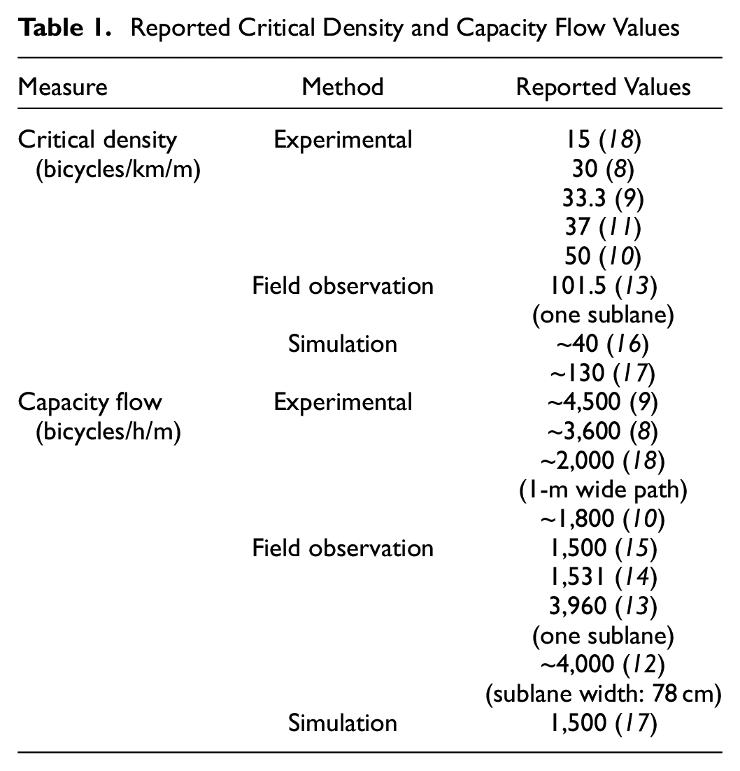
Based on field data, Botma and Papendrecht deduced a linear relation between mean speed and flow and a quadratic relation between flow and density ( 12 ). After accounting for speed and size in single-file systems, Zhang et al. identified a universal fundamental diagram for bicycle, pedestrian, and motor vehicle traffic and observed three traffic states: free-flow, congested, and stop-and-go waves ( 8 ). Guo et al. conducted a ring experiment in which cyclists were allowed to make full use of the width of the bicycle path to pass one another and found a higher critical density than Zhang et al. did in their single-file experiment ( 10 ). Li et al. observed both free-flow and congested conditions at four sites in China and were the first researchers to create a fundamental diagram containing both congested and free-flow states using only field data ( 13 ). The critical density reported by Li et al. is considerably higher than all values determined under experimental conditions. Hoogendoorn and Daamen proposed a composite headway model for bicycle traffic and derived model parameters using data from a busy intersection in Delft to estimate capacity flow ( 14 ). Navin analyzed the two-dimensional space requirements of child cyclists and observed free-flow conditions when the operating space was greater than 9.3 m²/bicycle ( 9 ). Congested conditions with no possibility for maneuvering the bicycle occurred at an operating space of less than 3.0 m²/bicycle. All of these analyses assume that bicycle traffic flow is uniform across the width of a bicycle path.

The total width of the infrastructure plays a critical role in bicycle traffic flow. Wierbos conducted a large-scale experiment in Delft to explore the relationship between average speed, flow, and density for various path widths ( 18 ). She found that the average speed and flow increase nonlinearly with path width while density decreases. She noted that a breakdown in traffic flow was not observed, despite conducting experiments with a narrow pathway and high-demand conditions. The hypothesis put forth by Wierbos is that cyclists anticipate congested conditions and adapt their behavior beforehand, allowing for the mitigation of potential breakdowns before they occur. Greibe and Buch found that the speed increases as the width of the path increases and the variation in speed decreases as the flow rate increases ( 15 ). Findings from previous studies, as well as the wide range of capacity flow and critical density in Table 1, could suggest that bicycle traffic flow depends on several factors in addition to the path width, including for example the slope ( 19 ), the composition of bicycle traffic ( 16 ), the curvature of the infrastructure, adjacent traffic/obstacles ( 15 ), pavement conditions, and cycling experience and culture.

A cyclist requires a certain amount of lateral space to operate their bicycle, known as “riding space” ( 3 ), which accounts for the physical width of the bicycle and for fluctuations in the lateral position that occur naturally while cycling. The riding space plus a “shy distance” or safety distance to obstacles adjacent to the bicycle infrastructure is the effective width of one bicycle sublane. The narrowest width of a bicycle sublane found in the literature is 0.75 m ( 20 ). Most papers and guidelines propose bicycle sublane widths of between 1 and 1.2 m ( 3 , 4 ). Sublane formation in bicycle traffic has also been observed in experiments and field studies. Wierbos observed the formation of sublanes at an infrastructure width of 2 m and found that the average speed is greater in left-hand sublanes than right-hand sublanes ( 18 ). Greibe and Buch observed bicycle traffic in Copenhagen and found that cyclists position themselves to the right-hand side of a bicycle path in low flow rate conditions (1 to 4 bicycles/10 s, 360 to 1,440 bicycles/h), and either form two sublanes (narrow bicycle paths) or distribute themselves over the width of the infrastructure (wide bicycle paths) in high-flow-rate conditions (>8 bicycles/10 s, >2,880 bicycles/h) ( 15 ). The relationships between flow, density, and average speed of bicycle traffic per sublane have not yet been explored using field, experimental, or simulation data.

We propose that a fundamental understanding of bicycle traffic flow that takes into account the nonuniformity of flow across the width of a bicycle path could provide an empirical foundation for determining the required width of bicycle facilities in demand-oriented contexts. The behavioral hypothesis that we work from is that cyclists hold to the right-hand sublane of a cycling infrastructure unless overtaking or riding in pairs/groups. Thus, as the bicycle traffic-demand-volume increases, the density increases first in the right-hand sublane and then this increase propagates through the center of the path to the left-hand sublane. The contributions of this paper are twofold: 1) the relationships between average speed, flow, and density per sublane are investigated and compared with relationships for the entire cross-section, and 2) the propagation of density across the width of a cycling infrastructure is quantified. Based on these results we propose a method for determining the number of sublanes necessary to serve a given bicycle traffic demand, To this end, we use cross-sectional data from a new generation of inductive loops for bicycle traffic that include the speed, direction, sublane, and timestamp accurate to 1 s from a sample of more than 1.3 million cyclists.

Methods

Sensor Technology

Data were collected using double inductive loop detectors for bicycle traffic. An inductive loop is a coil of electric wire installed slightly below or on the surface of a roadway or bicycle path and connected to a sensor. An electric current is passed through the loop, generating an electromagnetic field. Each time an object passes over the loop, the conductive material of the object influences the electromagnetic field. This technology has been used for decades to detect and count motor vehicle traffic and more recently for bicycle traffic. Bicycle traffic count data are typically stored in 15-min or 1-h intervals. Information about the individual crossings, such as speed, timestamp, direction, and lateral position is typically not collected or stored.

Cross-sectional data analyzed in this study were collected using ZELT^Evo inductive loop sensors. These diamond-shaped inductive loops count and classify bicycles, including carbon-framed bicycles and electric scooters. Inductive loops are manufactured for each cross-section and have widths between 80 cm and 1.4 m, roughly reflecting the widths of bicycle sublanes found in the literature. Multiple loops are installed beside each other on the cross-section, as shown in Figure 1 (Image B shows the inductive loops most clearly). In addition to classified count data, this system also allows for the recording of timestamps and thus the storage of individual crossings with speed, inductive loop ID, and direction of travel. The counting accuracy of the inductive loops is 95% for all potential situations, such as cyclists riding in groups or mixed traffic, and 99% of the speed observations lie within 1 km/h of the actual speed.

Figure 1.

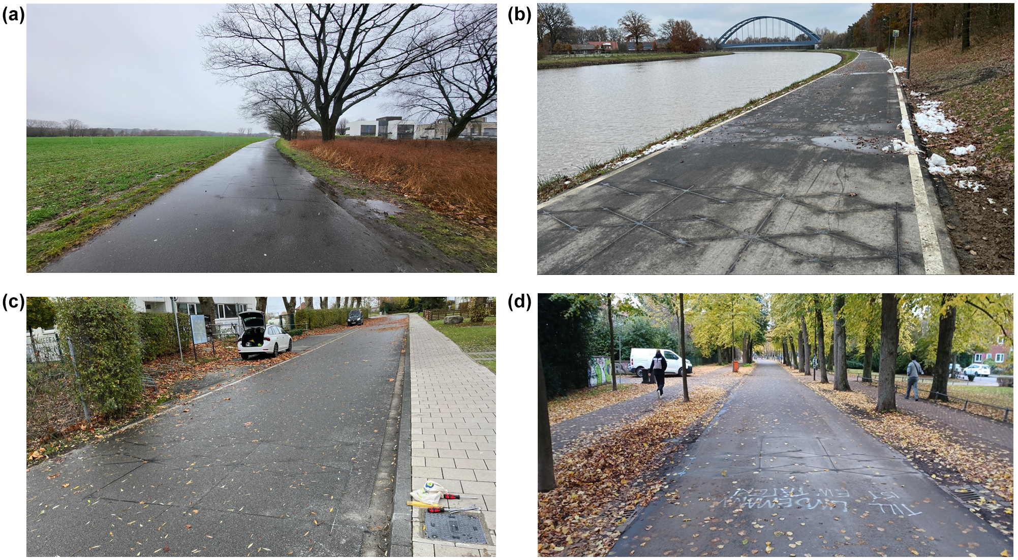
Inductive loop detectors at the sites: (a) Gasselstiege, (b) Kanalpromenade A, (c) Kanalpromenade B, and (d) Promenade.

Description of Sites

Data were collected in Muenster, Germany. Muenster is a medium-sized city with 315,000 inhabitants and a cycling modal split of about 30% of trips ( 1 ). Muenster is well-known in Germany for its well-developed network of cycling infrastructure, including wide on-road bicycle lanes, high-quality separated bicycle paths, and numerous bicycle streets (Fahrradstraßen). There are currently 23 permanent bicycle traffic counting sites in Muenster and up-to-date count data aggregated in 15-min time intervals is available online (opendata.stadt-muenster.de). In 2023, ZELT^Evo inductive loops were installed at 13 sites in Muenster, making it possible to collect extended count data containing the speed, direction, inductive loop ID, and timestamp for each crossing cyclist. This extended count data are not available online and are not collected continuously, as their collection and storage require significantly more energy than the 15-min aggregated count data.

Of the 13 cross-sections with ZELT^Evo counters, four sites were selected for data analysis (see Figure 1). The selection criteria were the bicycle traffic volume, the width of the infrastructure, and the distance from a traffic signal/intersection. The goal of this study was to assess bicycle traffic across the width of the bicycle path, without significant restrictions owing to the available width and with minimal influence from other types of road users. For this reason, separate bicycle paths with a minimum width of 3.5 m were selected. Although unidirectional bicycle lanes would have been preferable for our research question, all sites with a ZELT^Evo and a high traffic volume in Muenster are bidirectional. To account for this, we only included time intervals in our analysis in which there was no counterflow traffic. To ensure bicycle traffic was unaffected by stops and signal-induced platoons, sites were selected that were located more than 100 m from an intersection. Information about the four sites is summarized in Table 2.

Table 2.

Site Descriptions

Site	Cross-section width (m)	Number of loops/loop width (cm)	Max. flow rate^a (bicycles/h)	Total observations^b	Data collection dates (d/m/year)
Gasselstiege51°58′46.4″N, 7°36′23.3″E	3.6	3/120	3,600	287,932	19/2/2024 to 1/4/2024;6/5/2024 to 27/6/2024
Kanalpromenade A51°53′22.2″N 7°39′00.1″E	3.6	3/120	4,080	78,161	19/2/2024 to 1/4/2024;6/5/2024 to 27/6/2024
Kanalpromenade B51°58′46.2″N 7°39′47.5″E	4.4	3/145	2,880	146,694	19/2/2024 to 1/4/2024;6/5/2024 to 27/6/2024
Promenade51°57′24.7″N 7°37′28.2″E	4.2	3/140	3,000	846,571	19/2/2024 to 1/4/2024; 6/5/2024 to 19/6/2024

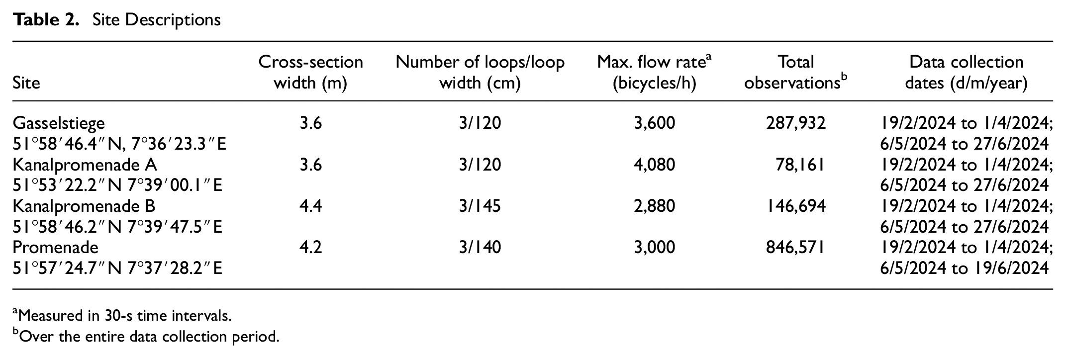
Measured in 30-s time intervals.

Over the entire data collection period.

Data Collection and Processing

Data were collected for 96 days during the first half of 2024, which was unusually wet and cool. The first collection campaign ran from February 19 to April 1, 2024. Data were collected in a second campaign from May 6 to June 27, 2024 in an effort to include more sunny, warm days with very high volumes of bicycle traffic in the sample. There was a technical issue storing data at the Promenade site at the end of June. Despite the generally cool weather, over 1.3 million cyclist crossings were included in the dataset and considerable bicycle traffic volumes were observed.

The raw data from the inductive loop detectors include the timestamp of the crossing accurate to 1 s, the inductive loop ID, the direction, and the speed. The inductive loop ID parameter indicates which of the three inductive loops registered the crossing. The raw data and the Python code used to process the data are available as a Github repository ( 21 ).

The speed data collected by the inductive loop detectors were irregularly binned. Bin widths of 1 km/h for speed observations less than 15 km/h (bins: 1, 2, …, 14 km/h); bin widths of 2 km/h for observations between 15 and 20 km/h (bins: 16, 18, and 20 km/h); bin widths of 4 km/h for observations between 21 and 28 km/h (bins: 24 and 28 km/h) were saved; and two bins captured high-speed observations above 30 km/h (bins: 36 and 48 km/h). Speed observations less than 7 km/h were removed from the dataset (between 1% and 3% of the data points were removed for each site).

To evaluate the accuracy of the speed observations, we compared the distribution of speeds measured at the Promenade site with the distribution reported by Brandenburg et al., who collected speed data using radar and video measurements on the Promenade facility in Muenster ( 16 ). They reported a normal distribution with a mean of 18.8 km/h and a standard deviation of 3.7 km/h across all the sites they observed (this appears to reflect the distribution for the Promenade site: Figure 3 of the Brandenburg et al. paper). As shown in Figure 2a, the two distributions match very well. Statistical testing indicated that although the means of the two distributions were significantly different, the effect size was small (t-statistic = 24.53, p-value = 0.000, Cohen’s d = 0.228). The speed distributions observed at all sites are shown in Figure 2b. An analysis of variance (ANOVA) test showed significant differences between the mean speeds observed at the different sites, but a negligible effect size (F-statistic = 4536.83, p-value = 0.000, $η^{2}$ = 0.010).

Figure 2.

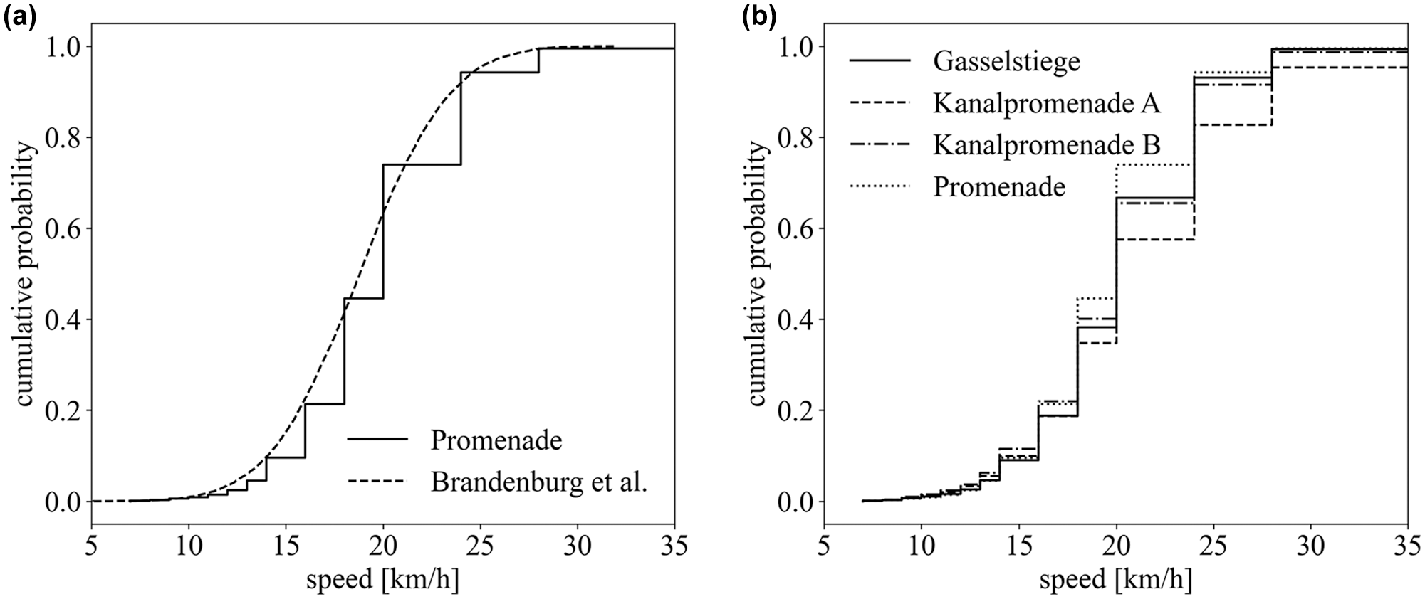
Comparison of the observed speed distribution at the Promenade site (both directions) and the distribution reported by (a) Brandenburg et al. ( 16 ), and (b) the speed distributions observed at each site.

The effect of weather on the observed speed distributions was assessed using the open weather and climate database Meteostat ( 22 ), which includes an hourly weather condition code for locations around the world. The 27 weather condition codes were aggregated into nine codes (“clear/fair,”“cloudy/overcast,”“fog,”“rain,”“sleet,”“snow,”“thunder and lightning,”“hail,”“storm”). Cyclists were detected in five weather conditions in our dataset. The observed speed distributions for each weather condition are shown in Figure 3a.

Figure 3.

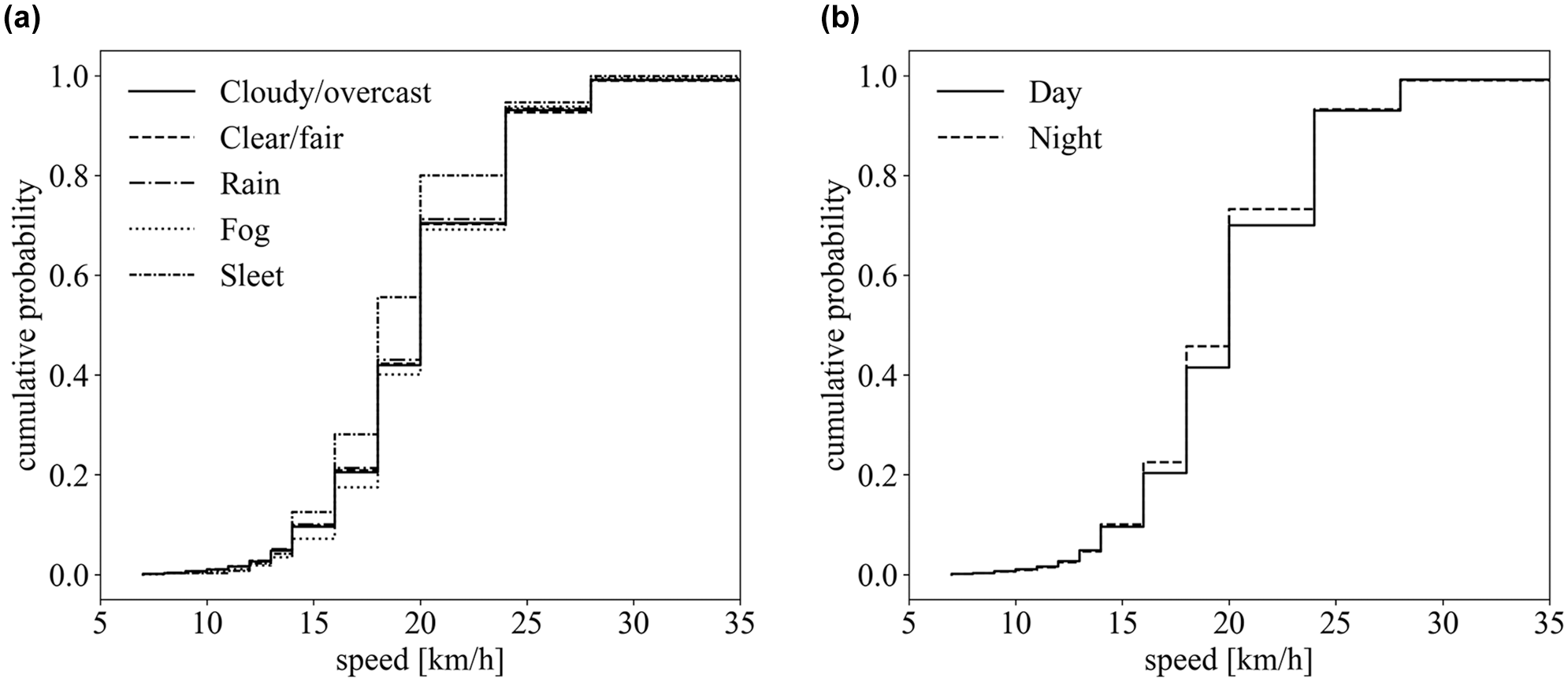
Observed speed distributions at all sites under (a) different weather conditions, and (b) during the day (6 a.m. to 7 p.m.) and night.

Cyclists tend to ride slower under sleet conditions and an ANOVA test showed that the mean speeds observed under different weather conditions were significantly different, although the effect size was negligible (F-statistic = 47.75, p-value = 0.000, $η^{2}$ = 0.000). Similarly, the distribution of speeds observed during daytime hours (between 6 a.m. and 7 p.m.) were compared with those observed during nighttime hours (Figure 3b). Cyclists rode slightly slower during the night and a t-test indicated that the mean speeds were significantly different with a negligible effect size (t-statistic = 25.57, p-value = 0.000, Cohen’s d = 0.060). Considering the negligible effect sizes of all tested independent variables (weather condition, day/night, location) on the speed distribution, it was decided to include all observations in one sample for the analyses.

The number of cyclists, $N_{l}$ , crossing each inductive loop, $l$ , in a given time interval, $T$ , was determined from the raw data. The flow rate, $q_{l}$ , passing inductive loop $l$ during the time interval T was calculated using Equation 1. The harmonic mean of the speeds, $\bar{v_{l}}$ , of all cyclists, $i$ , that passed loop $l$ in time interval $T$ was calculated using Equation 2. Under the assumption of stationary traffic conditions, the harmonic mean of observed speeds is equal to the space mean speed, which is used to compute traffic density from cross-sectional data. The density, $k_{l}$ , at inductive loop $l$ was derived from the space mean speed, $\bar{v_{l}}$ , the flow rate, $q_{l}$ , and the width of the inductive loop, $w_{l}$ (Equation 3). The total number of cyclists detected over the entire cross-section, $N$ , was the sum across all loops (Equation 4). The corresponding parameters across the entire cross-section, $q$ , $\bar{v}$ , and $k$ were calculated using the number of cyclists crossing the entire cross-section, $N$ , the speed, $v_{i}$ , of each cyclist, $i$ , and the total width of the bicycle path, $w$ .

q_{l} = \frac{N_{l}}{T}

(1)

\bar{v_{l}} = N_{l} {(\sum_{i = 0}^{N_{l}} v_{i, l}^{- 1})}^{- 1}

(2)

k_{l} = \frac{q_{l}}{\bar{v_{l}} * w_{l}}

(3)

N = \sum_{l = 1}^{3} N_{l}

(4)

Time intervals, $T$ , applied to bicycle traffic data in the literature range between 15 s ( 13 ) and 15 min ( 16 ). Different time intervals were tested on the data (10, 15, 30 s, and 1 min) and a time interval of 30 s was found to best capture rapidly changing flow conditions while smoothing out fluctuations from individual behavior.

Data were analyzed for each direction of travel on the bidirectional bicycle paths separately. For each direction, we calculated space mean speed, flow, and density parameters for bicycle traffic traveling in that direction, as well as the volume of counterflow traffic (cyclists moving in the opposite direction). All 30-s time intervals with counterflow traffic were removed from the sample for each site/direction dataset. Thus, our four sites effectively yielded eight datasets with unidirectional traffic.

Results

Despite the high modal split of cycling in Muenster, none of the flows observed at the sites approached the lowest estimates for capacity flow identified in the literature. The maximum flow rate at the Kanalpromenade A site was 4,080 bicycles/h (1,133 bicycles/h/m), which is considerably less than the 1,500 bicycle/h/m capacity flow estimated in previous research ( 14 , 15 , 17 ). Considering this, along with an analysis of the flow-speed and flow-density plots, we concluded that all observations reflected free-flow conditions. In this section, we present our analysis of the relationship between speed and flow rate as well as density and flow over the entire cross-section, and then differentiate by inductive loop. We then explore the propagation of density over the width of the bicycle path. All the flow rates presented are calculated by multiplying the number of cyclists counted in each 30-s observation time interval by 120.

Flow and Speed

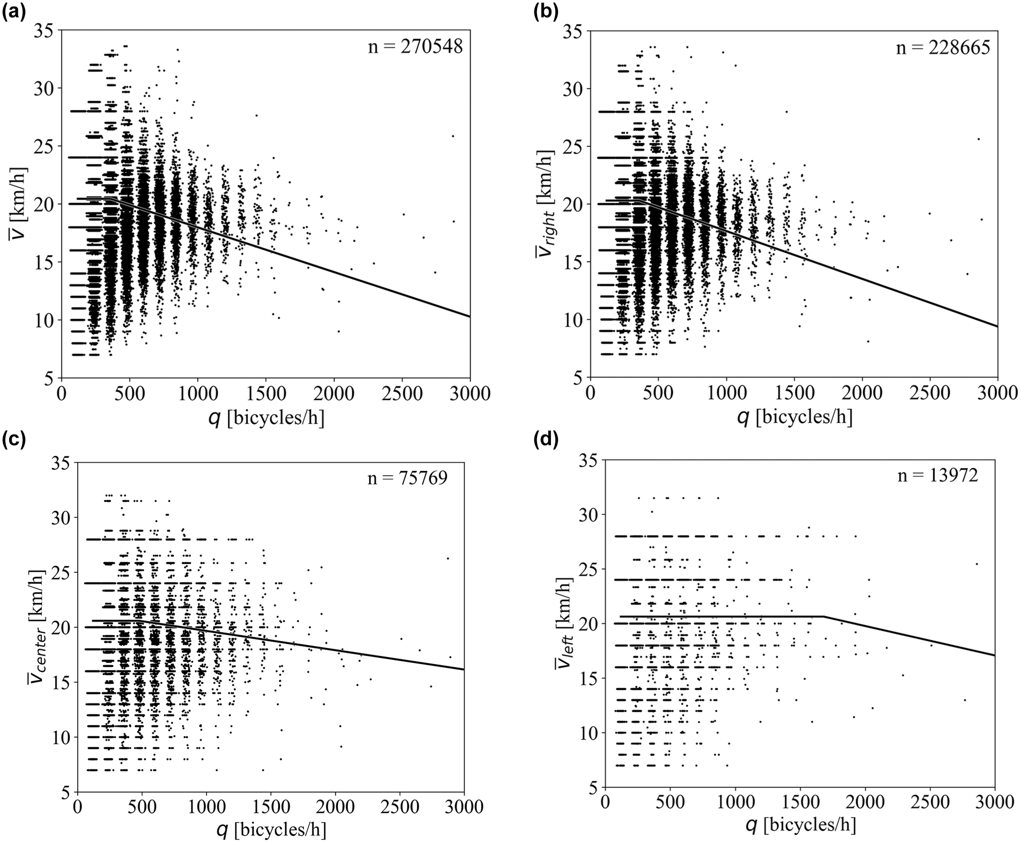
The space mean speeds and the flow rates observed in all 30-s observation time intervals for cyclists across the entire cross-section of the four locations are displayed in Figure 4a. The space mean speeds observed in the right, center and left inductive loops by the flow rate over the entire cross-section are shown in the top right (B), bottom left (C) and bottom right (D) of Figure 4, respectively. Note that the numbers of 30-s observation time intervals ( $n$ ) in the inductive loop figures are not equal and do not sum to the number over the entire cross-section (A) This is because only time intervals during which the given inductive loop registered any cyclists are included in Figure 4b to d . A jitter is applied to the data on the x-axis to increase the visibility of overlapping data points.

Figure 4.

(a) Space mean speed, $\bar{v}$ , and space mean speed per inductive loop, $\bar{v_{l}}$ ([b] right, [c] center, and [d] left) by the flow rate, $q$ , over the entire cross-section.

The space mean speed $\bar{v}$ appears to decrease slightly with the flow rate $\bar{q}$ over the entire cross-section (Figure 4a). The variation in mean speeds decreased with increasing flow rate. This was partially explained by the speeds of more cyclists being averaged in high-flow conditions, reducing the noise in the data. However, this may also indicate that cyclists ride at a more uniform speeds in high-flow conditions. As most cyclists were observed in the right sublane, the trends in the two top figures were quite similar. There was a less clear decrease in the mean or variation of the space mean speeds registered by the center and left inductive loops (Figure 4, c and d ) as the flow rate increased.

To identify trends in the data, we fit a piecewise linear model to the observations over the entire cross-section and for each inductive loop. The first piece was a horizontal line at the mean of the observed space mean speeds up to a breakpoint flow rate. After this point, a linear model was fit to the data. Different breaking points separating the horizontal line and linear model, ranging between 0 bicycles/h (purely linear model) and 2,000 bicycles/h, were tested and the most suitable breakpoint was selected based on the r² value. As shown in Figure 4, the best fit for data registered by the right-hand inductive loop was found with a horizontal line to 360 bicycles/h followed by a relatively strong decrease in space mean speed by flow rate, compared with the center and left inductive loops. The piecewise model fit to the data registered by the center inductive loop indicated a slightly later influence of flow rate on speed (at 480 bicycles/h) and a less pronounced decrease after this breakpoint. In the left-hand inductive loop, an effect of flow rate on space mean speed was first seen at 1,680 bicycles/h. More data in high-flow situations are needed to determine whether the trend after the breakpoint would be better captured using a curved rather than a linear model.

Flow and Density

The density across the entire cross-section and the flow rates observed in all 30-s observation time intervals at all four locations are displayed in Figure 5a. The densities calculated from data registered by the right, center, and left inductive loops by the flow rate over the entire cross-section are shown in Figure 5, b to d , respectively. 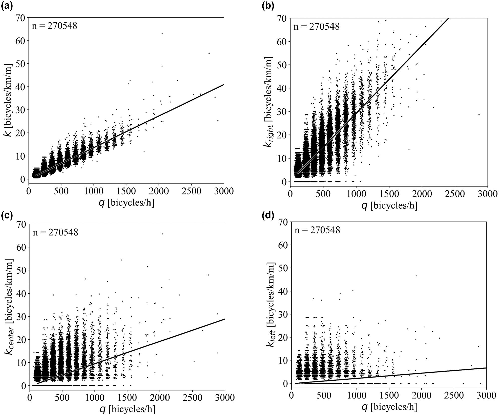Note that the number of 30-s observation intervals ( $n$ ) is equal across all figures, as a density of 0 bicycles/km/m was assigned to any time interval in which no cyclists were detected by the respective inductive loop. Again, a jitter was applied to the data on the x-axis to increase the visibility of overlapping data points.

Figure 5.

(a) Density, $k$ , and density per inductive loop, $k_{l}$ ([b] right, [c] center, and [d] left) by the flow rate, $q$ , over the entire cross-section.

As all observations describe free-flow conditions, the density, $k$ , was found to increase linearly with the flow rate, $q$ , over the entire cross-section (Figure 5a). The data showed relatively little variation, and a clear linear relationship between the variables was apparent over the entire cross-section. A much steeper relationship between the flow rate and density was observed on the right inductive loop compared with the other inductive loops. Although densities up to 70 bicycles/km/m were observed, we did not see an indication of a traffic breakdown taking place nor did we see a leveling of the density on the right-hand inductive loop that might indicate saturation on this inductive loop. This could suggest that many of the critical densities reported in the literature (Table 1) are low, particularly those stemming from experiments.

The form of the relationship between density and flow rate registered by the center and left-hand inductive loops was less clear. We hypothesized that the density on the center inductive loop is characterized by the presence of passing and pair-riding cyclists, even at low flow rates, whereas the relatively low densities observed on the left-hand inductive loop are related to the free-flow conditions governing on the right and center inductive loops.

Mapping Density Across the Width of the Bicycle Paths

As hypothesized, density was not uniform across a bicycle path, but built first on the right-hand side and progressed to the left. Heatmaps of the bicycle path were created to explore this progression for each direction of travel at the four sites separately (Figure 6). 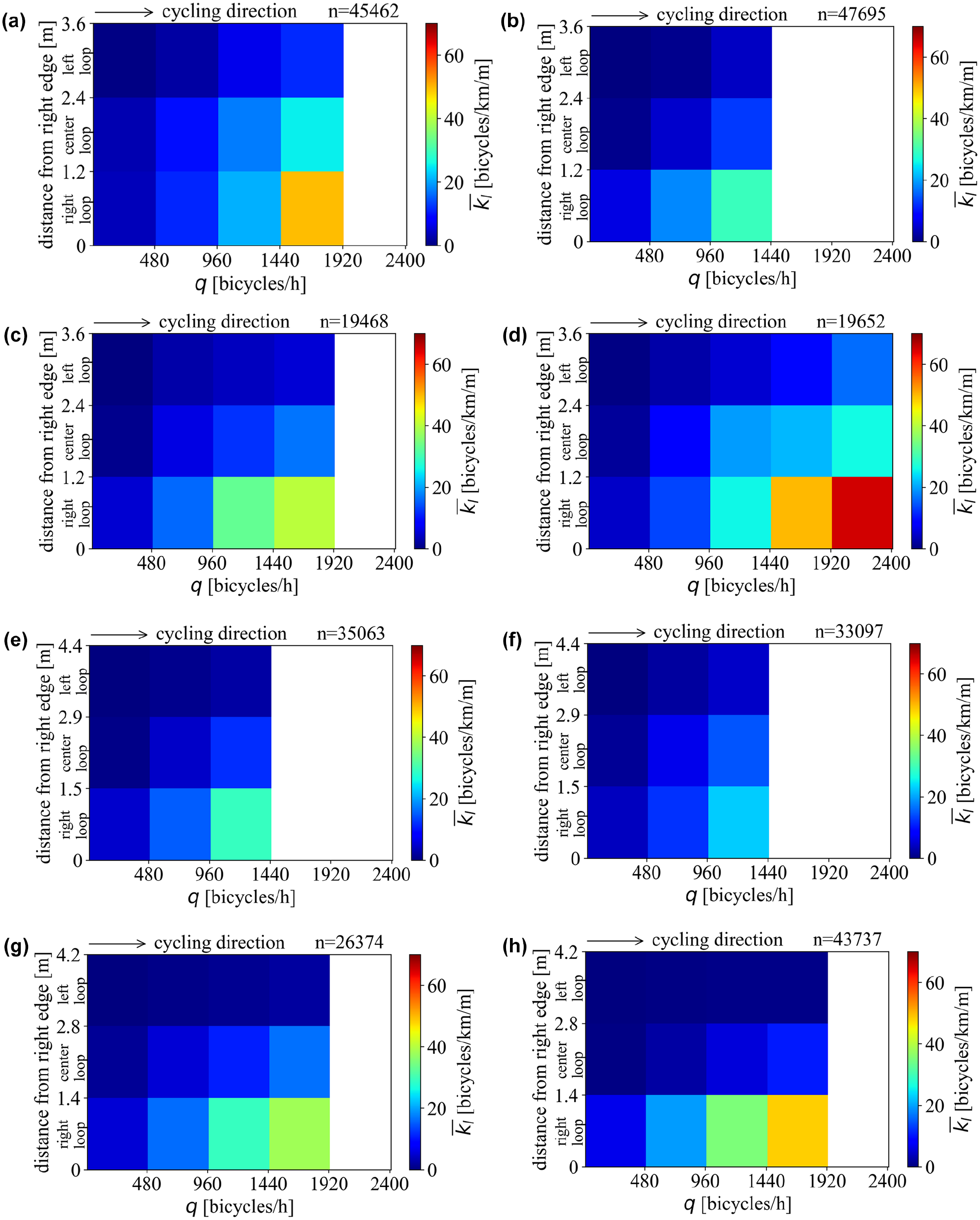To create the heatmaps, the observed densities per inductive loop for each 30-s time interval were sorted into bins depending on the overall flow rate, $q$ , at the cross-section. A bin width of 480 bicycles/h was selected to smooth the effects of traffic stochasticity while still showing trends in the data. This bin width was a multiple of 120 bicycles/h, which was important considering the length of the observation time interval. The mean density per inductive loop, $\bar{k_{l}}$ , for all 30-s time intervals in each bin was calculated. Means were only calculated if five or more 30-s intervals were observed in the bin. The nonuniform y-axis values in Figure 6 reflect the different path and inductive loop widths at the sites.

Figure 6.

The average density per inductive loop, $\bar{k_{l}}$ , by the flow rate, $q$ , over the entire cross-section at each site in each direction: (a and b) Gasselstiege; (c and d) Kanalpromenade A; (e and f) Kanalpromenade B; and (g and h) Promenade.

At all four sites, the density built first on the right-hand loop detector. Although there was variation between sites, density began to build on the center loop detector at about 1,200 bicycles/h. The two sites with wider loop detectors, Kanalpromenade B and Promenade, showed a building of density in the center at a higher flow and a more gradual increase in density in the center. None of the sites displayed moderate or high densities on the left-hand inductive loop.

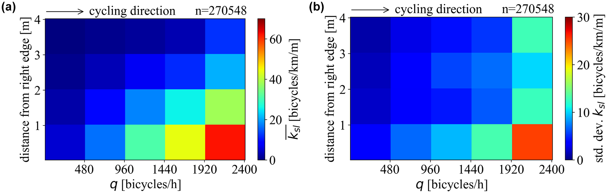
Bringing observations from all sites together requires creating sublanes of equal width. We assumed that the flow was distributed uniformly across the width of each inductive loop. The density in 1-m wide sublanes, $k_{sl}$ , was calculated using the weighted average of densities measured at the relevant inductive loops. All the observations were combined into one large dataset of cross-section flow rates and sublane densities. In Figure 7a, the mean and the standard deviation (Figure 7b) of the densities observed in all 30-s interval observations at all sites in both directions are shown.

Figure 7.

(a) Mean and (b) standard deviation of $k_{sl}$ across all sites in both directions.

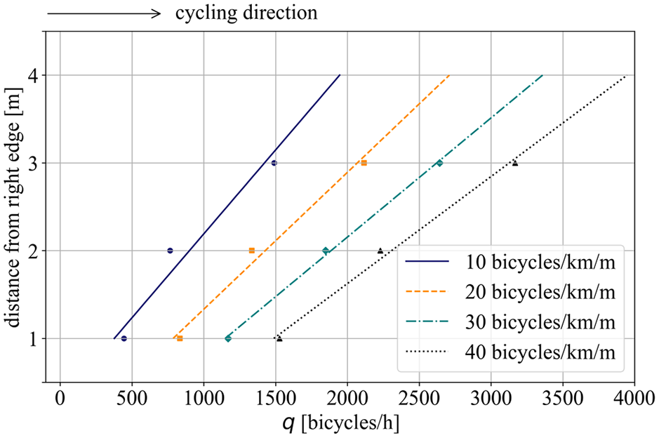
Linear interpolation of $\bar{k_{sl}}$ was performed along each of the 1-m wide sublanes. This interpolation allowed for the estimation of the flow at densities of 10, 20, 30, and 40 bicycles/km/m. These points were plotted for each density and sublane in Figure 8. Only very low densities occurred on the far left-hand sublane. This was partially because bidirectional bicycle paths were observed and cyclists avoided using the part of the infrastructure reserved for opposing traffic. This was likely to be true even though time intervals were removed in which opposing flow was present. For this reason, we omitted the interpolated points for the fourth sublane. Linear regression was used to derive a line of best fit through the interpolated points.

Figure 8.

Interpolated flow points for densities of 10, 20, 30 and 40 bicycles/km/m at each sublane and trendlines for the propagation of density.

Figure 8 illustrates the expected density at different widths (sublanes) of a bicycle path under different flow conditions. For example, at a cross-sectional flow of 1,000 bicycles/h, a density of ~25 bicycles/km/m is expected on the rightmost 1-m wide sublane and a density of ∼12.5 bicycles/km/m is expected on the second 1-m wide sublane. Any sublanes further to the left are expected to have a density below 10 bicycles/km/m.

The information displayed in Figure 8 was rearranged to demonstrate a possible approach for designing the widths of bicycle paths using the expected cross-sectional flow (Figure 9). Here, we assume that a minimum width of two sublanes (∼2 m) is necessary, regardless of demand, to ensure that cyclists can pass one another. Depending on the accepted maximum density on the leftmost sublane and the cross-sectional flow, the number of sublanes beyond this minimum can be determined.

Figure 9.

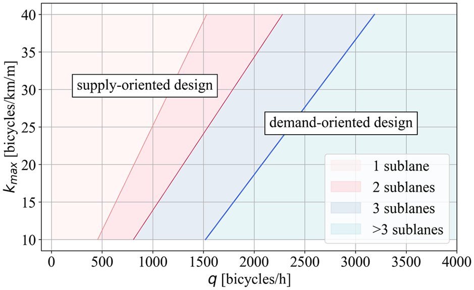
Approach for using the cross-sectional flow and design maximum density on the leftmost sublane to specify the necessary number of sublanes.

To demonstrate how Figure 9 can be used to select the width of a unidirectional bicycle facility, we set a maximum density of 10 bicycles/km/m on the leftmost sublane. According to Figure 8, on a three-sublane facility, the densities on the center and rightmost sublanes would be ∼19 bicycles/km/h and ∼35 bicycles/km/h, respectively. For situations with fewer than approximately 800 bicycles/h, supply-oriented provision of infrastructure with widths between 2.0 and 2.4 m (two sublanes) is sufficient. For demand volumes between 800 and 1,500 bicycles/h, widths between 3.0 and 3.6 m (three sublanes) are necessary, and for high-demand volumes of over 1,500 bicycles/h, widths between 4.0 and 4.8 m are recommended. For comparison, the widths suggested in the Danish design recommendations “The Concept for Cycle Superhighways” ( 5 ) are 2.25 to 2.5 m for low demand volumes less than 200 bicycles/h, 2.5 to 3.0 m for moderate demand volumes between 200 and 1,500 bicycles/h, and 3.0 to 3.5 m for high volumes of over 1,500 bicycles/h. These are the only guidelines we identified that contain demand variable widths for unidirectional bicycle facilities. Our findings suggest similar design widths at low volume conditions with a steeper increase in width for increasing demand volumes.

Discussion and Conclusion

This paper presents the first analysis of bicycle traffic flow differentiated by sublane of a bicycle path. We compared the relationships between mean speed, density, and flow across the entire bicycle path with the relationships on the right-hand, center, and left-hand sublanes. Our findings indicated that cyclists, as expected, held to the right side of a path, resulting in a steeper increase in density and a sharper drop in mean speed in the right-hand sublane as the overall flow increased. Only free-flowing bicycle traffic was observed; the maximum flows fell far below the capacity flows reported in the literature. However, subjective interpretations of the traffic situation in person, particularly at the Promenade site, indicated operation was near capacity during peak hours. We believe that more research is necessary concerning the perception of cyclists and the subjective criteria for “too full,” as measured by density rather than passing and meeting events. It could well be that the 40 bicycles/km/m limit suggested by Brandenburg et al. ( 16 ) is reasonable, but more research is necessary to quantify limits.

Our findings have several practical use cases. First, they could be used to inform practical approaches for dimensioning bicycle infrastructure in high-demand conditions, as demonstrated. This could be useful in setting recommended widths for unidirectional bicycle facilities in design guidelines such as the Urban Bikeway Design Guide or the German Recommendations for Bicycle Facilities (Empfehlungen für Radverkehranlagen). Here, it will be important to design for future bicycle traffic demand volumes, which can be derived by extrapolating trends in count data or using travel demand models. Our findings could also be useful in developing level of service evaluation methods based on density, which is more readily measurable than the number of passing and meeting events. These events form the basis of the current evaluation procedures in both the Highway Capacity Manual ( 23 ) and the German Manual for the Design of Road Traffic Facilities (Handbuch für die Bemessung von Straßenverkehrsanlagen) ( 24 ). However, it is necessary to quantify (or qualify) the density levels that are acceptable to cyclists first. Finally, our findings could be used to calibrate and validate microscopic traffic simulations of bicycle traffic.

This paper presents the first analysis of cross-sectional data from inductive loops for bicycle traffic that contain timestamps, speeds, and inductive loop ID for each crossing cyclist. However, some limitations should be considered. First, we only observed bidirectional bicycle infrastructure. Although we omitted time intervals with any traffic flow in the opposing direction, cyclists most likely remained on their side of the path. Finally, the width of the infrastructure itself constrains the cyclists’ behavior. We purposely selected wide infrastructure, but cyclists could have been compressed to the right-hand side of the path in higher volume conditions. The analysis of wide, one-way bicycle paths with high volumes of bicycle traffic would have been optimal for the research presented in this paper. However, we could not identify such locations in Germany. Another limitation is the inability of the inductive loop detectors to differentiate between conventional bicycles, cargo bikes, bicycles with trailers, and electrically supported bicycles. This diversity in bicycle form has a known impact on bicycle traffic flow (see for example Botma and Papendrecht [ 12 ]) that could not be further investigated using these data.

In the future, it will be necessary to continue investigating high-volume bicycle traffic situations as they become more common in the field. Observations at multiple sites with various infrastructure characteristics (width, directionality, slope, curvature, pavement, etc.) and bicycle traffic compositions are necessary to understand the influence of each of these parameters on the overall flow. It is necessary to gain an understanding of the subjective evaluation of different flow conditions. How dense is too dense? In the lack of a clear tipping point from free-flow to congested bicycle traffic, the perceptions and subjective evaluation of cyclists are more important to consider in planning and design than for motor vehicle traffic.

Footnotes

Acknowledgements

The authors would like to thank the City of Muenster for their permission to use the data for this paper. Heather Kaths would like to thank Fred Hall for his valuable comments and suggestions.

Author Contributions

The authors confirm contributions to the paper as follows: study conception and design: H. Kaths, A. Roosta; data collection: J. Fischer, A. Roosta; analysis and interpretation of results: H. Kaths, A. Roosta, A. Pušica, T. Kathmann; draft manuscript preparation: H. Kaths, A. Roosta, J. Fischer, A. Pušica, T. Kathmann. All authors reviewed the results and approved the final version of the manuscript.

Declaration of Conflicting Interests

The authors declared no potential conflicts of interest with respect to the research, authorship, and/or publication of this article.

Funding

The authors disclosed receipt of the following financial support for the research, authorship, and/or publication of this article: This research was supported by the German Federal Ministry for Digital and Transport on the basis of a decision by the German Bundestag. Research was carried out within the research project NUErLast (Nutzen und Umsetzbarkeit von detektorbasierter Erfassung von Lastenrädern, 19F1124A).

ORCID iDs

Heather Kaths

Aboozar Roosta

Data Availability

The inductive loop data are available here:

Python code for analysis is available here:

ChatGPT was used sparingly to edit problematic sentences.

References

Nobis

Mobilität in Deutschland. MiD Analysen Zum Radverkehr Und Fußverkehr. https://bmdv.bund.de/SharedDocs/DE/Anlage/G/mid-analysen-rad-fussverkehr.html?nn=12830.

Pucher

Buehler

Cycling towards a More Sustainable Transport Future. Transport Reviews, Vol. 37, No. 6, 2017, pp. 689–694.

National Association of City Transportation Officials. Urban Bikeway Design Guide. Island Press, Washington, D.C., 2025.

FGSV. Empfehlungen Für Radverkehrsanlagen. ERA FGSV-284. Forschungsgesellschaft für Straßen- und Verkehrswesen, Köln, 2010.

Office for Cycle Superhighways. Path and Route Course of Cycle Superhighways. https://supercykelstier.dk/concept/design-and-build/path-and-route-course/. Accessed April 24, 2025.

FGSV. Hinweise Zu Radschnelleverbindungen Und Radvorrangrouten. H RVS FGSV 284/1. Forschungsgesellschaft für Straßen- und Verkehrswesen, Köln, 2021.

Gavriilidou

Wierbos

M. J.

Daamen

Yuan

Knoop

V. L.

Hoogendoorn

S. P.

Large-Scale Bicycle Flow Experiment: Setup and Implementation. Transportation Research Record: Journal of the Transportation Research Board, 2019. 5: 709–719.

Zhang

Mehner

Holl

Boltes

Andresen

Schadschneider

Seyfried

Universal Flow-Density Relation of Single-File Bicycle, Pedestrian and Car Motion. Physics Letters A, Vol. 378, No. 44, 2014, pp. 3274–3277.

Navin

F. P. D.

Bicycle Traffic Flow Characteristics: Experimental Results and Comparisons. ITE Journal, Vol. 64, No. 3, 1994, pp. 31–37.

10.

Guo

Jiang

Wong

S. C.

Hao

Q.-Y.

Xue

S.-Q.

M.-B.

Bicycle Flow Dynamics on Wide Roads: Experiments and Simulation. Transportation Research Part C: Emerging Technologies, Vol. 125, 2021, p. 103012.

11.

Jiang

M.-B.

Q.-S.

Song

W.-G.

Traffic Dynamics of Bicycle Flow: Experiment and Modeling. Transportation Science, Vol. 51, No. 3, 2017, pp. 998–1008.

12.

Botma

Papendrecht

Traffic Operation of Bicycle Traffic. Transportation Research Record: Journal of the Transportation Research Board, 1991. 1320: 65–72.

13.

Some Operational Features in Bicycle Traffic Flow. Transportation Research Record: Journal of the Transportation Research Board, 2015. 1: 18–24.

14.

Hoogendoorn

Daamen

Bicycle Headway Modeling and Its Applications. Transportation Research Record: Journal of the Transportation Research Board, 2016. 1: 34–40.

15.

Greibe

Buch

T. S.

Capacity and Behaviour on One-Way Cycle Tracks of Different Widths. Transportation Research Procedia, Vol. 15, 2016, pp. 122–136.

16.

Brandenburg

Geistefeldt

Zeidler

Buck

Vortisch

Baier

M. M.

A New Method for the Quality of Service Assessment of Highly Frequented Bicycle Facilities in Germany. Transportation Research Record: Journal of the Transportation Research Board, 2023. 2: 1288–1302.

17.

Gould

Karner

Modeling Bicycle Facility Operation. Transportation Research Record: Journal of the Transportation Research Board, 2009. 1: 157–164.

18.

Wierbos

M. J.

Macroscopic Characteristics of Bicycle Traffic Flow: A Bird’s-Eye View of Cycling. PhD dissertation. Delft University of Technology, 2021.

19.

Parkin

Rotheram

Design Speeds and Acceleration Characteristics of Bicycle Traffic for Use in Planning, Design and Appraisal. Transport Policy, Vol. 17, No. 5, 2010, pp. 335–341.

20.

Botma

Method to Determine Level of Service for Bicycle Paths and Pedestrian-Bicycle Paths. Transportation Research Record: Journal of the Transportation Research Board, 1995. 1502: 38–44.

21.

Heather Kaths. LoopDetectorData. GitHub, 2024. https://github.com/HeatherAnne85/LoopDetectorData.

22.

Meteostat. Wetterrückblick Und Klimadaten. https://meteostat.net/de/. Accessed October 30, 2024.

23.

National Academies of Sciences, Engineering, Medicine, and Transportation Research Board. Highway Capacity Manual 7th Edition: A Guide for Multimodal Mobility Analysis. National Academies Press, Washington, D.C., 2022.

24.

FGSV. Handbuch Für Die Bemessung Von Straßenverkehrsanlagen. HBS FGSV 299. Forschungsgesellschaft für Straßen- und Verkehrswesen, Köln, 2015.

Mapping Bicycle Traffic Flow Across the Width of a Bicycle Path to Inform Facility Design

Abstract

Keywords

Methods

Sensor Technology

Description of Sites

Data Collection and Processing

Results

Flow and Speed

Flow and Density

Mapping Density Across the Width of the Bicycle Paths

Discussion and Conclusion

Footnotes

Acknowledgements

Author Contributions

Declaration of Conflicting Interests

Funding

ORCID iDs

Data Availability

References