Sage Journals: Discover world-class research

Abstract

This article investigates the effect of ambient light level on traffic flow for different types of road user—pedestrians, cyclists, and drivers of motorized vehicles—using counts of traffic flow recorded by automated counters. Previous analyses have focused only on pedestrians and/or cyclists, in Arlington, Virginia (U.S.) and Birmingham (U.K.). The new data represent all three types of road user for one location (Cambridge, U.K.) and motorized vehicles in London (U.K.), Adelaide (Australia) and trunk roads in England. The effect of ambient light level was established using odds ratios to compare traffic flows in case and control hours, chosen to isolate the effect of ambient light from other factors of influence. The data for this analysis included the counts for 71,477,159 motorized vehicles, 89,392 pedestrians, and 66,925 cyclists. It was found that darkness leads to significant reductions in pedestrians and cyclists but does not have a significant effect on the number of motorized vehicles.

Keywords

operations traffic flow theory traffic flow characteristics traffic flow pedestrians bicycles human factors human factors of infrastructure design and operations lighting safety motorcycles mopeds pedestrian safety bicyclist safety

The need to travel persists across changes in ambient light level, from daylight to darkness. This article investigates the influence of ambient light on the number of road users present. Changes in ambient light are expected to influence travel decisions because, after dark, the visual system is impaired, including reductions in contrast discrimination and depth perception, and an increase in reaction time ( 1 ). Darkness significantly increases the risk of some types of road traffic collision (RTC) compared with daylight, which may be at least partially attributable to darkness-related visual impairment ( 2 , 3 ). A better understanding of how change in ambient light level influences traffic flow would inform consideration of the potential benefits of road lighting after dark, including how the change in RTC risk is influenced by any changes in exposure.

The Department for Transport describes daily and seasonal variations in travel for the U.K. ( 4 ). On weekdays, the daily pattern for cars is bimodal (Figure 1), with peak traffic flows around 08:00 and 17:00 as expected because of the typical working day, but a broad unimodal peak on weekends between about 09:00 and 16:00. (Martin shows a similar bimodal peak for the hourly annual average traffic flow [1997–1998] for motorways in France [ 5 ]). In relation to seasonal trend (Figure 2), the average hourly traffic flow for cars is fairly uniform across the year but with a slight increase in summer, while for cycles the seasonal variation is more significant with miles traveled being 75% higher in the summer months than in winter months. These data are used for basic traffic flow analyses and do not isolate the impact of a single factor on travel behavior.

Figure 1.

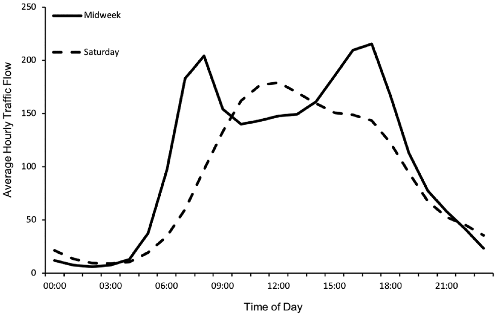
Daily car traffic trends for midweek (Tuesday, Wednesday, Thursday) and Saturday for 2018 as published by the U.K. Department for Transport ( 6 ).

Figure 2.

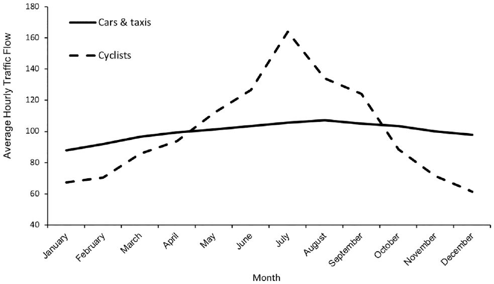
Monthly vehicle traffic trends for cars and taxis and cyclists between 2014 and 2016 as published by the U.K. Department for Transport ( 7 ).

To isolate the impact of ambient light from other factors which influence the number of road users, this work applies the approach previously used to study the influence of ambient light on RTCs ( 2 , 3 ). Travel counts for the days before the twice-yearly daylight-savings clock change are compared with those for the days following clock change. The counts are recorded within a specific daily time window, chosen so that it is daylight before the clock change but dark after the clock change (or vice versa, depending on whether spring or autumn). Comparing travel counts in daylight and darkness for the same time of day is done with the assumption that this isolates the change in ambient light level from other factors which may affect travel decisions, such as the purpose and/or destination of the journey. Changes in travel count between daylight and darkness are compared with simultaneous changes in control periods using an odds ratio (OR). These control periods are either permanent daylight or permanent darkness before and after the clock change. Including control periods within the OR accounts for seasonal influences on traveler count such as the weather.

Three types of road user are considered: pedestrians, cyclists, and drivers of motorized vehicles.

First, consider pedestrians. After dark, and generally at lower light levels, pedestrian reassurance is reduced, and a lower level of reassurance is associated with reduced walking ( 8 – 11 ). Darkness is known to reduce the likelihood of people leaving their homes, in particular the elderly, a result of their perceived vulnerability and concerns about the speed and volume of traffic after dark ( 12 ). It is therefore expected that, for a given time of day, there would be fewer pedestrians after dark than in daylight.

This expectation was confirmed by analyses of pedestrian data from Arlington, Virginia, U.S., over a 6-year period from 2011 to 2016. The number of automated traffic counters changed over this period, with nine automated counters in Autumn 2011 and 22 counters in Spring 2016 (Table 1). When the analysis considered the 13 days before and after clock change, the OR of 1.72 (95% CI = 1.69–1.75, p < 0.001) suggested a significant reduction in pedestrian numbers after dark ( 13 ). (Note that these are the OR for the early day and late dark control hours in that study: see Uttley and Fotios, and Robbins and Fotios for analyses of how the choice of control hour influences the OR [ 13 , 14 ]). When these data were further analyzed using the whole year approach, the OR of 1.93 (95% CI = 1.92–1.95, p < 0.001) again revealed significantly fewer pedestrians after dark ( 15 ). The whole-year method uses data from all 52 weeks rather than the (just under) 8 weeks used in the clock-change method, and employs seasonal variation in solar altitude to establish periods of darkness and daylight for the same time of day.

Table 1.

Past Studies Using Odds Ratios (ORs) to Compare Travel Counts in Different Ambient Light Levels

	Data		Method of analysis			Road user	OR (95% confidence interval [CI]) for effect of darkness on travel count**
Study	Location and period	Reported count interval	Period analyzed	Case hour	Control hours	Road user
Uttley and Fotios ( 13 )	Arlington, Virginia, U.S., 2011–2016	15 min	Clock change (2 weeks before/after)	Spring: 18:00–18:59 Autumn: 17:00–17:59	Spring: 16:30–17:29; 19:30–20:29; 14:30–15:29; 21:30–22:29 Autumn: 15:30–16:29; 18:30–19:29; 13:30–14:29; 20:30–21:29	PedestriansCyclists	1.72 (1.69–1.75) p < 0.0011.42 (1.41–1.44) p < 0.001
Fotios et al. ( 15 )	Arlington, Virginia, U.S., 2012–2015	15 min	Whole year	18:00–18:59	15:00–15:59; 21:00–21:59	Pedestrians	1.93 (1.92–1.95) p < 0.001
						Cyclists	1.67 (1.66–1.68) p < 0.001
Uttley et al. ( 16 )	Birmingham, U.K., 2012–2015	60 min	Whole year	18:00–18:59	14:00–14:59; 22:00–22:59	Cyclists	1.32 (1.31–1.33) p < .001

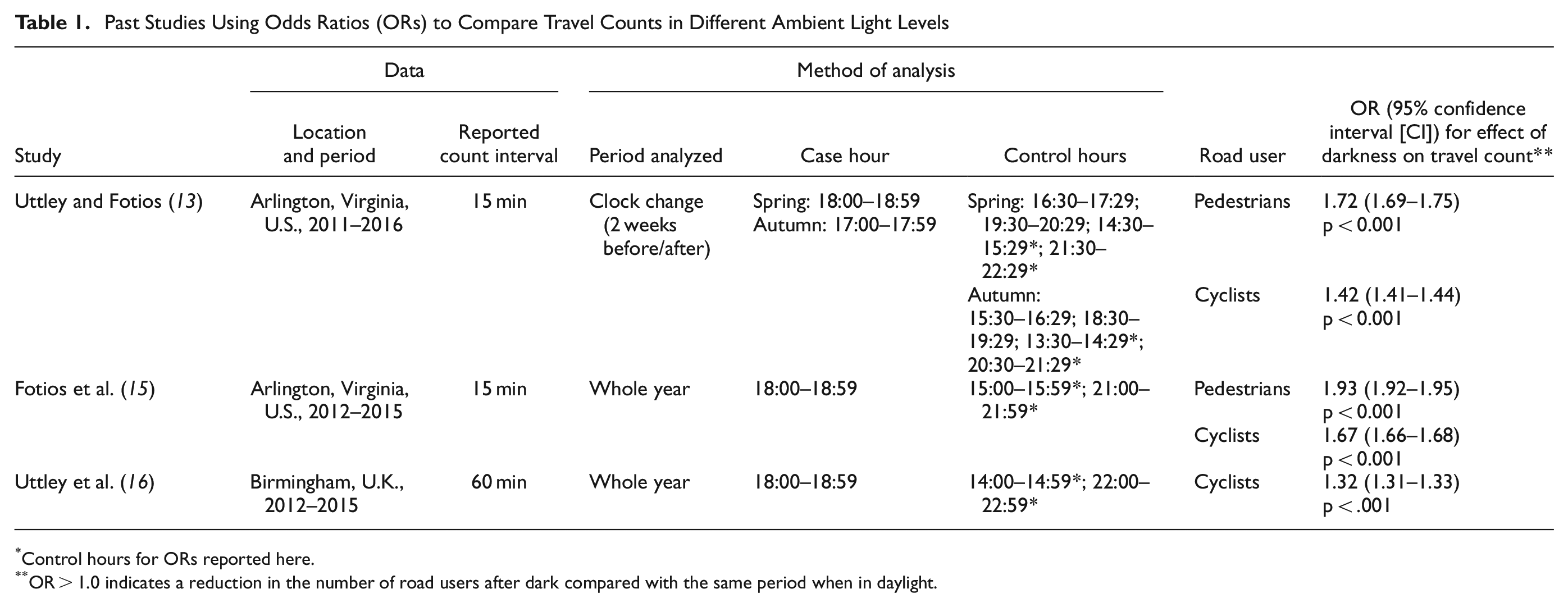
Control hours for ORs reported here.

OR > 1.0 indicates a reduction in the number of road users after dark compared with the same period when in daylight.

In some locations, cycling is considered to be a dangerous mode of transport. For example, the 2017 British Social Attitudes Survey found that 62% of cyclists think it is too dangerous to cycle on U.K. roads ( 17 ). Cycling after dark is considered to be more dangerous than cycling in daytime because of the apparent reduced visibility to others ( 18 ). It is therefore expected that, for a given time of day, there would be fewer cyclists after dark than in daylight. The data from Arlington, Virginia, U.S., also included counts of cyclists, and analyses of these revealed significant reductions of cyclists after dark using both the clock-change method (OR = 1.42, 95% CI = 1.41–1.44, p < 0.001) and the whole-year method (OR = 1.67, 95% CI = 1.66–1.68, p < 0.001) ( 13 – 15 ). Uttley et al. used the whole-year method to analyze cyclist count data from a further location (Birmingham, U.K.) and found the same effect, reporting an OR of 1.32 (95% CI = 1.31–1.33, p < 0.001) ( 16 ).

If fewer people are walking or cycling after dark, the remainder must be doing something else instead. Consider three possibilities. First, they are making the same journey but instead driving using a personal motorized vehicle: darkness is a suggested factor in the choice of travel mode for short trips ( 19 ). Second, they are again making the same journey but using some form of shared motorized transport for some part of it, such as sharing a private vehicle or using public transport. Third, they are not leaving their home. This could be investigated by repeating the ambient light level analysis for motorized vehicles in addition to pedestrians and cyclists. Ideally, this investigation would be conducted for all types of road user within the same area. Such investigation does not yet appear to have been reported.

Tenekeci et al. investigated the effect of ambient light level on the number of motorized vehicles ( 20 ). They counted vehicles on the 13 approaches (37 entry lanes) to four roundabouts in Leeds, U.K. Surveys were conducted in 1999 at saturated flow times (defined as vehicles queueing to enter the roundabout) under the four combinations of ambient light level (day or dark) and weather condition (dry or wet): day-dry, day-wet, dark-dry, and dark-wet. Compared with the day-dry condition, the least reduction was found for dark-dry condition (6.3%) and the greatest reduction for the dark-wet condition (10.8%). There are three limitations with these data. First, the definitions of day and dark were not reported; light conditions were apparently recorded but were not included in this publication. Second, the four roundabouts were located on A-roads, which are usually major roads, and may not include those journeys which would otherwise be carried out by walking or cycling. Third, the study did not report whether the 6.3% reduction in traffic because of light conditions was a statistically significant reduction.

The effect of ambient light level on motorized traffic has been studied by others, but with a focus on vehicle speed rather than vehicle numbers. Jägerbrand and Sjöbergh investigated the effect of ambient light on passenger vehicle speed and truck speed using hourly count data from 25 automated counters in Sweden over the years 2012 to 2014 ( 21 , 22 ). Their analyses did not suggest an effect of ambient light on vehicle speed.

Current knowledge of the influence of ambient light level on travel counts for different types of road user is therefore limited because there are only few studies, and these consider data for different road users in different locations rather than a common location. The current article examines the influence of ambient light on the number of pedestrians, cyclists, and motorized vehicles. Count data for all three user groups for one location (Cambridge, U.K.) are analyzed. Those data include only 14 locations and for a limited period (June 2019–September 2020). To extend the data set, motorized vehicle count data from two urban locations (Adelaide, Australia, and London, U.K.) is also analyzed. For commuting journeys, short distances are associated with a greater tendency to walk ( 23 ). Similarly, changes in ambient light level might be expected to affect the decision to walk, cycle, or drive for short journeys, but less likely to be the case for long journeys. Therefore, vehicle count data on trunk routes from the main road network in England is also analyzed. Table 2 shows how these new analyses extend the existing data set.

Table 2.

Past and Planned Studies of Travel Counts in Different Ambient Light Levels

Location	Road users counted
Location	Pedestrians	Cyclists	Motorized vehicles
Current analyses
Cambridge, U.K.	✓	✓	✓ (urban)
Adelaide, Australia	na	na	✓ (urban)
London, U.K.	na	na	✓ (urban)
England, U.K.	na	na	✓ (trunk roads)
Previous analyses
Arlington, Virginia, U.S.*	✓	✓	na
Birmingham, U.K.**	✓	✓	na

Uttley and Fotios, and Fotios et al. ( 13 , 15 ).

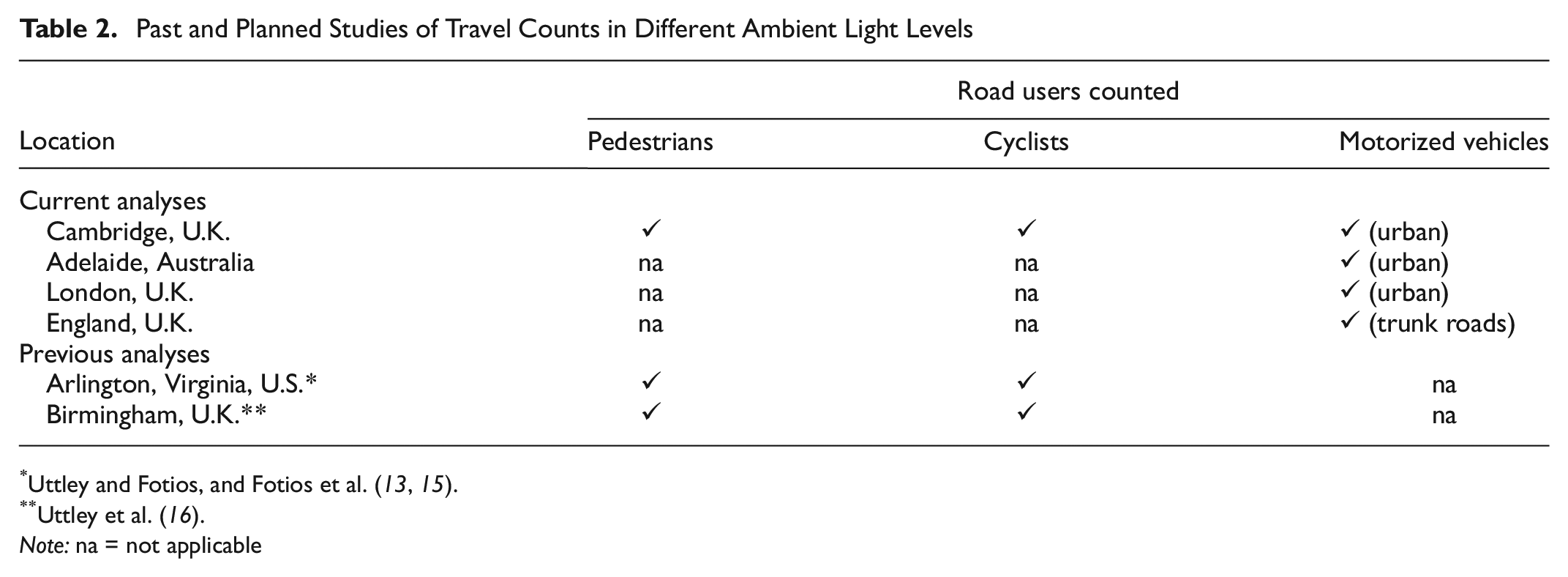
Uttley et al. ( 16 ).Note: na = not applicable

Method

Data Sets

Table 3 shows the locations, road user types, and counter details for the data used in the current analyses. All data used in this analysis are openly available online, apart from those for London.

Table 3.

Summary of Travel Count Data Sets

Location	Road user*	Data
Location	Road user*	No. of locations	Count interval	Date range for which counts available
Cambridge, U.K.	Pedestrians, cyclists, and motorized vehicles (urban)	14	60 min	Jun 3, 2019–Sep 30, 2020
Adelaide, Australia	Motorized vehicles (urban)	118	60 min	Jan 1, 2010–Dec 31, 2014
London, U.K.	Motorized vehicles (urban)	2	60 min	Jan 1, 2015–Dec 31, 2016
England, U.K.	Motorized vehicles (trunk roads)	14	15 min	Jan 1, 2018–Dec 31, 2019

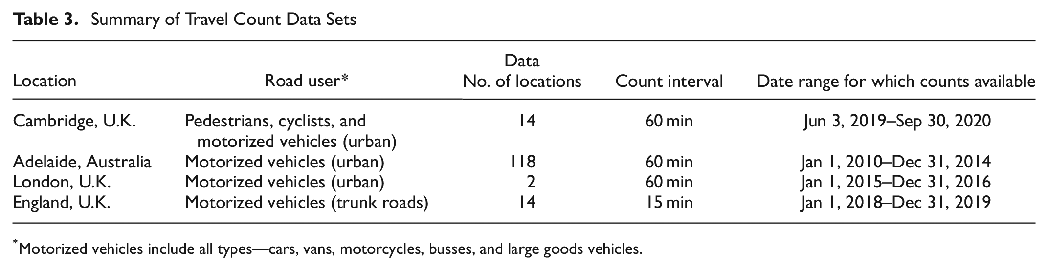
Motorized vehicles include all types—cars, vans, motorcycles, busses, and large goods vehicles.

For the city of Cambridge, U.K., traffic counters in 14 locations provide separate data for motorized vehicles (including cars, busses, goods vehicles, and motorcycles), pedestrians, and cyclists. These data are openly available on the Cambridgeshire Insight Open Data website: https://data.cambridgeshireinsight.org.uk/dataset/mill-road-project-traffic-sensor-data. The 14 counters were located on minor, urban roads near the city centre and the data used were for the period Jun 3, 2019–Sep 30, 2020. The longitude and latitude of the 14 locations can be seen in Supplementary data 1. All counters recorded traffic heading in north and south directions, which, for the current analysis, were combined.

For Adelaide, there are publically available data from 122 automatic traffic counters located at signalized intersections and pedestrian crossings throughout the metropolitan region: https://data.sa.gov.au/data/dataset/traffic-intersection-count ( 24 ). These counters include 69 at four-way signalized intersections, 30 at signalized T-junctions, and 23 at signalized pedestrian crossings, located on minor, urban roads near the city centre. Site identification numbers, as well as longitude and latitude of these locations, can be seen in Supplementary data 2. For the 54 counters that included two directions of traffic, these were combined for the current analysis, providing one count of hourly traffic at that location regardless of traffic direction. Traffic flow data were available at hourly intervals over the 5-year period 2010–2014. Data cleaning revealed that data were missing for the autumn weeks in 2010 for four of the counters, and therefore these counters were removed leaving 118 counters being used for the current analysis.

Transport for London (TfL) in the U.K. has automatic traffic counters located in central and outer London, and from these report average daily counts. For the current work, traffic counts at hourly intervals were provided, by private communication, for only two counters, situated in the outer London areas of Barking and Dagenham for the 2-year period 2015–2016. These counters were located on minor, urban roads. The longitude and latitude of the two counters were 51.53105, 0.07229 and 51.52916, 0.08570. Both counters recorded traffic heading in north and south directions, which for the current analysis were combined.

Traffic counters for Adelaide, Cambridge, and London were located on minor roads in urban areas. A person might choose to drive after dark if they thought it was unsafe to walk or cycle. Such a change might be seen by counters located in urban areas, but is less likely to be seen on trunk roads where walking or cycling is not an option regardless of the ambient light level. Additional counts of motorized vehicles were therefore sought for main trunk roads in England. These data are publicly available from Highways England and were retrieved from: http://tris.highwaysengland.co.uk/detail/trafficflowdata. Highways England operate over 10,000 automatic traffic counters, with several counters placed at different locations along each road. For this analysis, seven roads were chosen at random, and on each of these roads, two counter locations were chosen at random, thus giving 14 counters to match that available for Cambridge. The seven roads included four motorways and three A-roads. In the U.K., A-roads tend to be trunk roads—the major roads which connect major destinations such as cities, ports and airports. Data were extracted for these 14 locations for the years 2018 and 2019. Details of the roads, years, and location descriptions (including GPS reference and direction of traffic flow), as well as longitude and latitude for each location, can be seen in Supplementary data 3.

Data Processing

For each data set, count data were extracted for 7 days before and after the spring and autumn clock changes. The clock change date always falls on a Sunday morning, just after midnight. Therefore, the first 7 days were Sunday to Saturday before the clock change, and the second 7 days were Sunday to Saturday after the clock change.

A 1 h case period was identified, such that it was in darkness one side of the clock change date, and daylight during the same hour on the other side of the clock change date (Table 4). Phases of ambient light are defined according to solar altitude, with daylight being a solar altitude of greater than 0° and darkness (for land-based application) a solar altitude of less than −6° (39). These times were identified using the sunset times given for each location by the Time and Date website ( 25 ). The case hours for London and Cambridge were the same. The case hour for Adelaide was different because of its latitude. The data from the trunk roads in England are reported at 15 min intervals, which allowed for the case hour to be more precisely chosen.

Table 4.

The Case and Control Periods for Autumn and Spring Clock and the Change in Ambient Light Condition

Location	Period	Spring	Autumn	Ambient light before/after clock change
Cambridge, U.K.	Case	18:00–18:59	17:00–17:59	Dark-day (spring)
	Case	18:00–18:59	17:00–17:59	Day-dark (autumn)
	Control day	14:00–14:59	14:00–14:59	Day-day (spring and autumn)
	Control dark	21:00–21:59	21:00–21:59	Dark-dark (spring and autumn)
London, U.K.	Case	18:00–18:59	17:00–17:59	Dark-day (spring)
	Case	18:00–18:59	17:00–17:59	Day-dark (autumn)
	Control day	14:00–14:59	14:00–14:59	Day-day (spring and autumn)
	Control dark	21:00–21:59	21:00–21:59	Dark-dark (spring and autumn)
Trunk roads in England	Case	18:30–19:30	16:45–17:45	Dark-day (spring)
	Case	18:30–19:30	16:45–17:45	Day-dark (autumn)
	Control day	14:00–14:59	14:00–14:59	Day-day (spring and autumn)
	Control dark	21:00–21:59	21:00–21:59	Dark-dark (spring and autumn)
Adelaide, Australia	Case	19:00–19:59	18:00:18:59	Dark-day (spring)
	Case	19:00–19:59	18:00:18:59	Day-dark (autumn)
	Control day	14:00–14:59	14:00–14:59	Day-day (spring and autumn)
	Control dark	21:00–21:59	21:00–21:59	Dark-dark (spring and autumn)

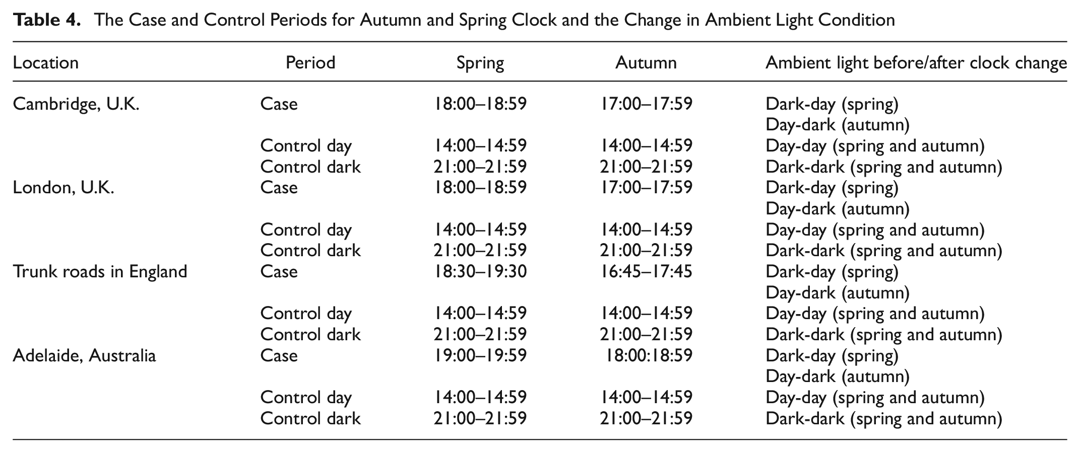
Two 1 h control periods were also identified. A control period has the same ambient light condition before and after the clock change. Two control periods were chosen, with one being daylight (14:00–14:59) and the other after dark (21:00–21:59). These two control periods can be seen in Table 4, along with the ambient light condition before and after the clock change.

Analysis

Travel count data were analyzed using an OR ( 26 – 28 ). For each road user type, an OR and associated 95% confidence interval (CI) were calculated for the overall traffic count, comparing the changes before and after the clock change in the case period with the two control periods. The autumn and spring clock change periods were combined to produce an overall OR. The OR was calculated using Equation 1, and the 95% CI using Equation 2. This OR gives a measure of the change in the number of motorized vehicles, cyclists, or pedestrians associated with daylight conditions compared with darkness conditions.

OR = CaseDay / CaseDark / ContolDay / ControlDark

(1)

C I = e x p (Ln (OddsRatio) \pm 1.96 \times \sqrt{\frac{1}{CaseDay} + \frac{1}{CaseDark} + \frac{1}{ControlDay} + \frac{1}{ControlDark}})

(2)

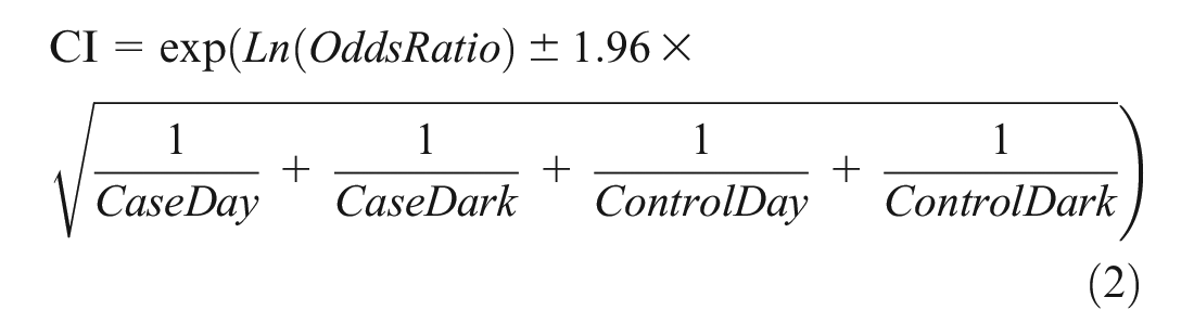
where

CaseDay is the number of motorized vehicles, cyclists, or pedestrians in the case period before the autumn clock change and after the spring clock change;

CaseDark is the number of motorized vehicles, cyclists, or pedestrians in the case period after the autumn clock change and before the spring clock change;

ControlDay is the number of motorized vehicles, cyclists, or pedestrians in the control periods on days when the case period would be in daylight;

ControlDark is the number of motorized vehicles, cyclists, or pedestrians in the control periods on days when the case period would be in darkness.

Results

Table 5 shows the travel counts for Adelaide, London, Cambridge, and trunk roads in England and for motorized vehicles, pedestrians, and cyclists for the case and control periods. Also shown are the ORs, 95% Cis, and significance of the departure of the OR from unity as calculated using a Chi-square test. An OR significantly (p < 0.05) greater than 1.0 suggests a significant reduction in traffic after dark—that there is more traffic in daylight conditions than dark for the same time of day. An OR significantly (p < 0.05) less than 1.0 suggests that there is less traffic in daylight conditions than darkness. An OR not significantly different from 1.0 suggests that any departure from unity is not statistically significant and, therefore, that there is no effect of ambient light level.

Table 5.

The Summated Counts for Five Locations for Either Motorized Vehicles, Pedestrians, or Cyclists for the Case and Control Periods as Well as the Odds Ratios (ORs), 95% Confidence Intervals (CIs), and Significance

Location	Road user type	Period	Season	Clock change	Light condition	Total traffic count	OR (95% CI)	p-value
Adelaide, Australia	Motorized vehicles	Case	Autumn	Before	Light	6,353,263	1.001 (1.000–1.002)	p = 0.74
			Autumn	After	Dark	6,348,672
			Spring	Before	Dark	4,589,557
			Spring	After	Light	4,715,472
		Control	Autumn	Before	Light	11,366,064
			Autumn	After	Dark	11,120,145
			Spring	Before	Dark	11,182,623
			Spring	After	Light	11,181,857
London, U.K.	Motorized vehicles	Case	Autumn	Before	Light	177,296	1.003 (0.997–1.009)	p = 0.31
			Autumn	After	Dark	170,305
			Spring	Before	Dark	147,283
			Spring	After	Light	147,729
		Control	Autumn	Before	Light	289,420
			Autumn	After	Dark	292,906
			Spring	Before	Dark	250,343
			Spring	After	Light	264,774
Cambridge, U.K.	Motorized vehicles	Case	Autumn	Before	Light	75,224	0.97 (0.96–0.98)	p < 0.001
			Autumn	After	Dark	79,155
			Spring	Before	Dark	25,589
			Spring	After	Light	20,801
		Control	Autumn	Before	Light	115,650
			Autumn	After	Dark	117,706
			Spring	Before	Dark	45,165
			Spring	After	Light	37,843
	Pedestrians	Case	Autumn	Before	Light	17,847	1.29 (1.26–1.33)	p < 0.001
			Autumn	After	Dark	14,156
			Spring	Before	Dark	5,386
			Spring	After	Light	4,715
		Control	Autumn	Before	Light	16,868
			Autumn	After	Dark	18,568
			Spring	Before	Dark	6,429
			Spring	After	Light	5,423
	Cyclists	Case	Autumn	Before	Light	15,834	1.57 (1.52–1.62)	p < 0.001
			Autumn	After	Dark	10,504
			Spring	Before	Dark	3,544
			Spring	After	Light	4,127
		Control	Autumn	Before	Light	10,931
			Autumn	After	Dark	12,652
			Spring	Before	Dark	4,610
			Spring	After	Light	4,723
Trunk roads in England	Motorized vehicles	Case	Autumn	Before	Light	332,476	0.989 (0.984–0.994)	p < 0.001
			Autumn	After	Dark	335,630
			Spring	Before	Dark	199,894
			Spring	After	Light	201,836
		Control	Autumn	Before	Light	333,564
			Autumn	After	Dark	332,418
			Spring	Before	Dark	310,969
			Spring	After	Light	315,530

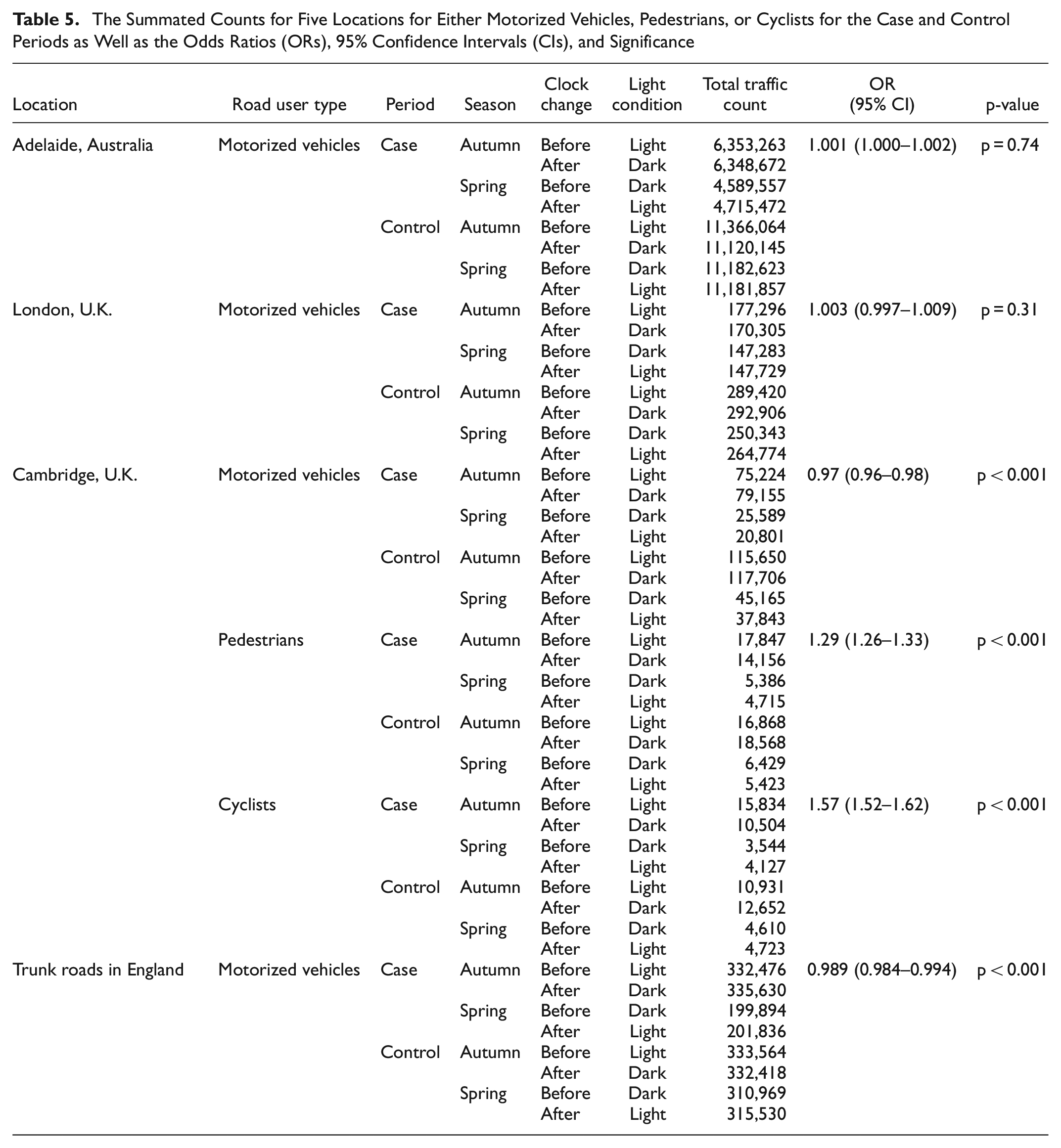
For motorized vehicles, the travel counts recorded in Adelaide and London do not suggest a significant effect of ambient light. However, while OR for the travel counts recorded in Cambridge and on trunk roads in England suggest a significant reduction in motorized vehicles after dark, these do not reach the threshold (1.22) even for small effect sizes ( 29 , 30 ). The ORs for pedestrians and cyclists are in the range of small (1.22) to medium (1.86) effect sizes.

Discussion

Travel choices after dark

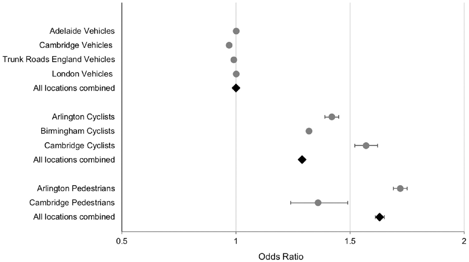
Analysis of the effect of ambient light level on the number of pedestrians, cyclists, and motorized vehicles for one location, Cambridge, suggests that darkness leads to a significant reduction in the number of pedestrians and cyclists and a significant but negligible increase in motorized vehicles. The generalizability of these findings was examined by comparison with counts of motorized vehicles in three other locations (Adelaide, London, and trunk roads in England) and previous analyses of pedestrians and cyclists in two other locations (Arlington, Virginia, U.S. and Birmingham, U.K.) (Table 6, Figure 3). The findings appear to be consistent across locations.

Table 6.

Combined-Location Analysis of the Effect of Ambient Light Level on Flows of Motorized Vehicles, Cyclists, and Pedestrians, with Odds Ratios (ORs) and 95% Confidence Intervals (CIs) Reported for All Studies

Road user and location	Individual locations	Locations combined
Road user and location	OR (95% CI)	OR (95% CI)	p-value
Motorized vehicles
Adelaide, Australia	1.00 (1.00, 1.00)	1.00 (0.999, 1.001)	p = 0.86
Cambridge, U.K.	0.97 (0.96, 0.98)
Trunk roads in England	0.99 (0.98, 0.99)
London, U.K.	1.00 (1.00, 1.01)
Cyclists
Arlington, Virginia, U.S.	1.42 (1.41, 1.44)	1.29 (1.28, 1.30)	p < 0.001
Birmingham, U.K.	1.32 (1.31, 1.33)
Cambridge, U.K.	1.57 (1.52, 1.62)
Pedestrians
Arlington, Virginia, U.S.	1.72 (1.69, 1.75)	1.63 (1.61, 1.65)	p < 0.001
Cambridge, U.K.	1.29 (1.26, 1.33)

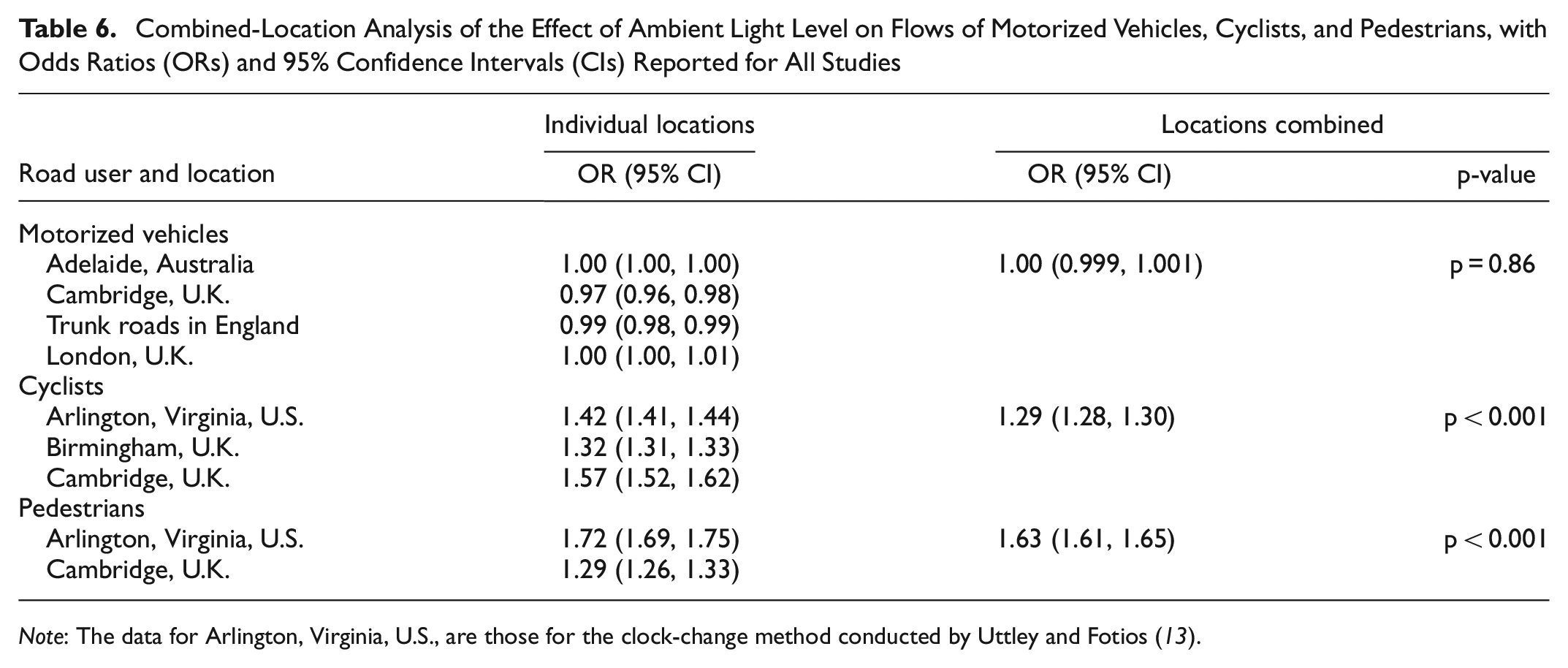
Note: The data for Arlington, Virginia, U.S., are those for the clock-change method conducted by Uttley and Fotios ( 13 ).

Figure 3.

ORs (and 95% CIs) established for current and previous analyses of effect of ambient light on flows of motorized vehicles, cyclists, and pedestrians.

Results from the current and previous analyses suggest that after dark there are significant reductions in the number of people walking (p < 0.001) or cycling (p < 0.001) compared with the same time of day but when in daylight. Results from the current study do not suggest that ambient light level has a significant effect on counts of motorized traffic, for either urban roads or trunk roads (Table 6, Figure 3). While the OR for motorized vehicles in specific locations may suggest a significant difference (Table 5) the effect size is negligible. This is in contrast to a previous study which indicates a 6.3% reduction in the amount of traffic after dark ( 20 ). This discrepancy may arise from differences in the manner by which daylight and darkness were defined, which was not reported by Tenekeci et al., and therefore the expected reduction in vehicle numbers with later time in the evening (Figure 1) will have confounded their comparison of daylight versus dark ( 20 ).

Reduced active travel (walking or cycling) after dark is not matched with an increase in motorized vehicles. This supports the third option raised in the introduction that fewer people are leaving their homes after dark.

After dark, drivers of motorized vehicles should use headlights. These reduce the impairment of darkness to drivers’ vision and may offset any reluctance to drive after dark. Cyclists also have front lights, although usually of much lower luminous intensity and spread than those of vehicle headlights. Pedestrians could carry a torch but this is not common. If the effect of reduced ambient light is mitigated by headlights, then the OR would be smallest for motorized vehicles, larger for cyclists, and largest for pedestrians. This is the pattern indicated by the results, with Table 6 and Figure 3 revealing an overall OR of unity for vehicles, and ORs of 1.29 and 1.63 for cyclists and pedestrians, respectively.

The decision to walk, cycle, or drive can depend on the purpose of the journey. Handy defined walking trips as being “strolling” or “destination,” or a combination of the two ( 31 ). Strolling trips are optional trips, without particular destinations, as might be undertaken for exercise or fresh air. Destination trips are those taken with a motivation to arrive at a specific destination. Combination trips are those motivated by both the desire to stroll and the desire to arrive at a particular destination. For destination trips, feasibility (i.e., the practicality or viability of walking, whether the arrival/departure time is flexible, availability of other travel modes), and accessibility (i.e., distance) factors may affect the choice between walking or driving, while for strolling trips, feasibility and safety (i.e., fear of crime) factors may affect the choice between taking a walk, changing the time at which a walk is taken, or not leaving the house at all ( 32 ).

This is confirmed by Foster et al. who found that increased fear of crime led to reduced leisure walking (Handy’s strolling trips) but not transport-related walking (Handy’s destination trips) ( 11 ). One explanation for the reduction in the number of pedestrians after dark is, therefore, that these were strolling walks—optional walks that were not taken because people tend to feel less safe walking after dark than during the daytime ( 8 , 9 , 31 ). Nair et al. describe four types of cycling trip: commute, school, social, and exercise ( 33 ). Of these, the first two might be considered as destination trips and unaffected by ambient light level, whereas the latter two might be considered as strolling or leisure trips and more likely to be avoided after dark because of safety concerns. Unfortunately, the nature of the current data, being counts of each type of road user without further personal information, does not permit differentiation of trip purpose that would otherwise inform the discussion. While trip purpose could be established by questioning each traveler, this would be unlikely to reach the sample sizes possible with automated counters.

A decision to not walk or cycle may contribute to social isolation where that journey is not made instead by motorized vehicle. Social isolation may be of particular significance for females, with one study finding 63% of the sample reporting that after dark they would avoid going out alone by foot ( 34 ). Similarly, the elderly are less likely to walk after dark if they perceive it to be less safe, and this is particularly so for recreational walking (i.e., strolling or leisure trips) ( 35 , 36 ).

An obvious response to the problem that darkness is a deterrent for travel by walking and cycling is to install road lighting. The presence of road lighting enhances reassurance to walk after dark, variations in the characteristics of lighting affect the degree of reassurance offered, and a lower level of reassurance is associated with reduced walking ( 8 – 11 , 37 ). Thus, installing road lighting in a previously unlit area, or improving the lighting in a previously lit area, may lead to more walking and cycling and a reduction in social isolation. This has been demonstrated for cyclists, with analysis of cyclist counts in Birmingham, U.K., alongside estimates of road brightness from aerial imagery, suggesting that higher road brightness, to a point, is associated with a reduction in the reduction of cyclists after dark ( 16 ). Such data can be used to support and encourage cycling after dark. However, this association remains to be validated in other locations and for other road users. Any change in road lighting also needs to consider the effect on other visual tasks and benefits of road lighting ( 38 ). There is also a need to consider the unwanted consequences of road lighting, including sky glow, ecological impact, and energy consumption. A better understanding of the benefits of road lighting helps the lighting designer to balance the costs and benefits.

Civil Twilight

Ideal travel count data would enable the ambient light level to be precisely established, thus to distinguish between the main phases of ambient light—daylight, darkness, and civil twilight. Civil twilight is the partially daylit periods immediately before morning sunrise and immediately after evening sunset, defined as the period where solar altitude lies between 0° and −6° ( 39 ). In this period, daylight persists because of the reflection and scattering of sunlight toward the horizon of a terrestrial observer, and is generally sufficient to enable outdoor civil activity to continue unhindered without resorting to the use of electric road lighting ( 39 ). Some studies omit data within civil twilight to isolate collisions that occur at darkness, and avoid the ambiguity of the twilight period ( 2 , 40 , 41 ). If civil twilight is not omitted but retained, it leads to an underestimate of the difference between daylight and darkness ( 42 ).

Establishing solar altitude requires knowledge of the location of the traffic flow counter, and the date and time of each counted item. Previous investigations have tended to analyze secondary data—the outputs of travel counters installed by municipal and highways authorities—and these report the data in bins, typically of 1 h interval. Discrimination of travel counts in daylight, twilight, and dark periods is therefore limited by the intervals at which count data are binned. Jägerbrand and Sjöbergh used data at 1 h intervals and classified these according to the light condition of the middle of the interval, that is, at the 30 min point ( 21 ). They state: “if an interval was mostly daylight but had a few minutes of twilight, it was classified as daylight.” Pedestrian and cyclist count data from Arlington, Virginia, U.S., were available in 15 min bins, enabling better account of the times of sunset and sunrise, although, following Johansson et al., that analysis did not omit civil twilight but included it within the dark period ( 13 , 43 ).

The current analysis used a defined case hour to compare darkness and daylight, with this case hour being defined by the time of sunset or sunrise (0° solar altitude) rather than civil twilight (−6° solar altitude). While it is possible to more precisely characterize events occurring in daylight or darkness at the same time of day, this requires that events are collated at intervals of sufficiently precision, which means less than 1 h ( 41 , 42 ). The data used for three locations in the current analysis (Table 3) were available only at hourly intervals. This is expected to produce a conservative estimate of the effect of ambient light ( 42 ). Methods which more precisely distinguish between darkness and daylight generally produce a larger OR.

Control Hours

In this analysis, the intervals between the control periods and case periods ranged from 1 to 4 h, according to season and location (Table 2). This was done to maintain control hours at a constant time of day (starting at either 14:00 or 21:00) in an attempt to capture the same types of journey. Analysis in previous work of traffic flow suggests the case-control interval can influence the estimated effect of ambient light ( 13 ). Specifically, the OR was 1.72 for a case-control interval of 150 min and 1.56 for an interval of 30 min. This may be a spillover or displacement effect, with a control period which is closer in time to the case period potentially including individuals whose decision to walk or cycle was influenced by the knowledge that the ambient light level was about to change.

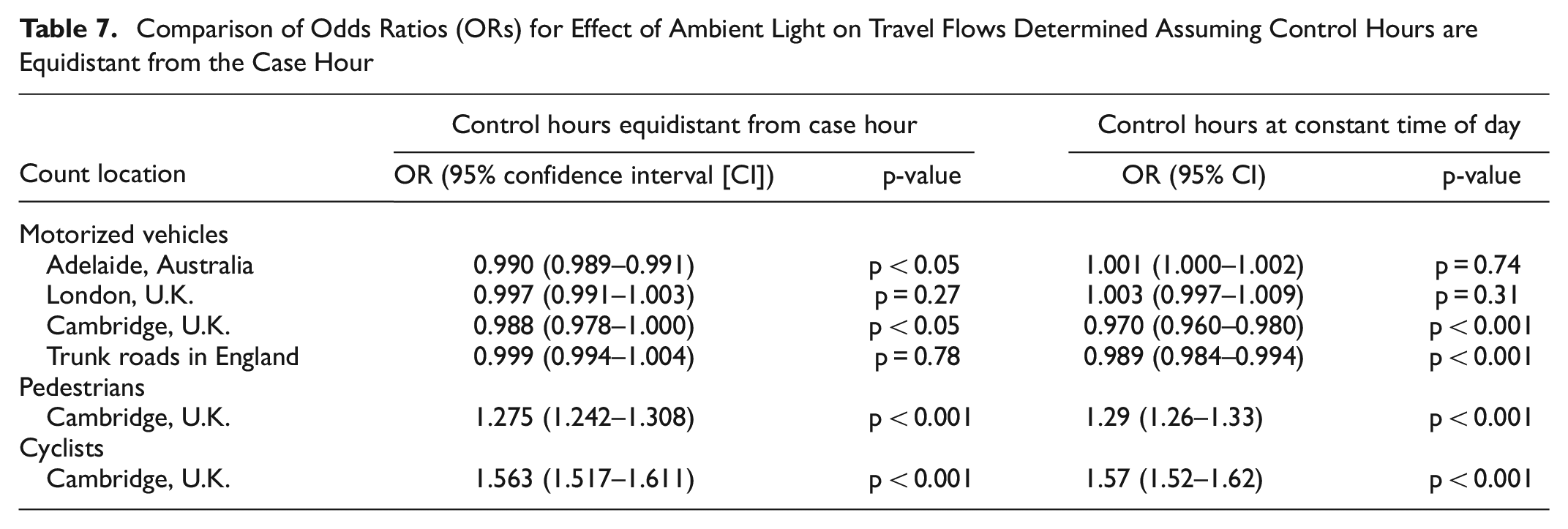
The differing case-control periods incurred in the current analysis may have affected the estimated ORs. To check this, a further analysis was conducted using a consistent interval (2 h) for all combinations of season and location: day control periods ended 2 h before the case hour commenced, and dark control periods started 2 h after the end of the case hour. Average durations of walking and car journeys in the U.K. are suggested to be 12 min and 36 min, respectively ( 44 ). A 2 h interval either side of the case hour is therefore unlikely to be confounded by spillover or displacement effects of ambient light, as suggested by Uttley and Fotios ( 13 ). Supplementary data 4a shows the case and control hours for Adelaide, London, Cambridge and the trunk road network in England, and Supplementary data 4b shows the total traffic counts and the ORs. As can be seen by the summary of this analysis (Table 7), the ORs for all locations are similar to the original analysis. The difference from unity is suggested to be significant for motorized vehicles in Adelaide and Cambridge (p < 0.05) but not for London and the trunk road network in England (p = 0.27, p = 0.78, respectively). The original analysis (above) with control periods chosen to maintain constant times of day rather than constant case-control intervals suggested significant differences for Cambridge and the trunk road network in England, while Adelaide and London did not suggest to be different from unity. While this alternative analysis suggests some small changes in statistically significant effects, in all four locations the OR is very close to unity for all analyses.

Table 7.

Comparison of Odds Ratios (ORs) for Effect of Ambient Light on Travel Flows Determined Assuming Control Hours are Equidistant from the Case Hour

Count location	Control hours equidistant from case hour		Control hours at constant time of day
Count location	OR (95% confidence interval [CI])	p-value	OR (95% CI)	p-value
Motorized vehicles
Adelaide, Australia	0.990 (0.989–0.991)	p < 0.05	1.001 (1.000–1.002)	p = 0.74
London, U.K.	0.997 (0.991–1.003)	p = 0.27	1.003 (0.997–1.009)	p = 0.31
Cambridge, U.K.	0.988 (0.978–1.000)	p < 0.05	0.970 (0.960–0.980)	p < 0.001
Trunk roads in England	0.999 (0.994–1.004)	p = 0.78	0.989 (0.984–0.994)	p < 0.001
Pedestrians
Cambridge, U.K.	1.275 (1.242–1.308)	p < 0.001	1.29 (1.26–1.33)	p < 0.001
Cyclists
Cambridge, U.K.	1.563 (1.517–1.611)	p < 0.001	1.57 (1.52–1.62)	p < 0.001

Limitations

When counting motorized traffic, the nature and location of available counters vary in the likelihood of counting other modes of transport. While it is possible that the counters located in London may have included cyclists, this contamination is unlikely in other locations. For Adelaide, 84% of the counters were positioned on roads where there was a separate cyclist lane, with these cycle lane counts not included in the current data. It is therefore assumed that there will be minimal cyclist counts in the included data, as previous large-scale studies in the U.S. have found that if cycle lanes are available, cyclists will tend to use these designated lanes ( 45 , 46 ). For Cambridge, travel flow was provided separately for motorized vehicles and cyclists, and for the trunk road network in England it is extremely unlikely that cyclists would be using trunk roads compared with local roads ( 47 ). This analysis was conducted using data from traffic counters installed by others: in further work there may be a benefit in giving further consideration to precise locations of counters or to bespoke installation of new counters.

It may be expected that weather conditions would influence travel decisions, in particular leisure trips rather than destination trips ( 48 ). The data used for the current analyses do not include weather information. One analysis of motorized vehicles in Scotland suggests that the effects of extreme and unseasonal weather tend to be small (< 5%) with the exception being a reduction in traffic of up to 15% for snow lying on the road surface ( 49 ). The decision to walk or cycle is influenced by both temperature and precipitation ( 50 – 53 ). Precipitation may lead to a large-scale switch from active travel, where people are exposed to the elements, to motorized vehicles, where people are protected from the weather, and is one of the most important reasons not to cycle ( 48 ). For the current focus, the question is whether weather conditions would affect investigation of the influence of ambient light level. The use of control periods within the OR should offset any effect of weather, unless the weather was consistently different for the case and control periods: previous analysis suggests that it does not have significant effect investigations of walking and cycling ( 13 ). A more precise account of the influence of weather on travel counts could be made using a multivariate analysis if weather data (e.g., temperature, precipitation, cloud cover, and wind speed) were available for the locations, dates, and times of each count.

It is suggested above that reduced active travel (walking or cycling) after dark implies that fewer people are leaving their home after dark. An alternative explanation is that these pedestrians and cyclists instead chose to travel at a different time of day. A comparison of such personal choice might be investigated in further research using travel diaries.

Conclusion

This article explored the effect of ambient light on traffic counts, using automated counters located in urban areas (Cambridge, Adelaide, London) and on trunk roads in England. The analysis exploited the twice-yearly clock change to compare traffic counts in case hours which were daylight before the clock change but dark afterwards (or vice versa). ORs were established to show the changes in travel count for the case hour with simultaneous control periods which were either permanently dark or permanently lit for the period of analysis, thus isolating the effect of ambient light level from seasonal variations such as weather.

These data suggest a small and statistically significant reduction in the number of pedestrians and cyclists after dark. For motorized traffic, the effect was of negligible size and overall was not suggested to be statistically significant. If some people are not walking or cycling after dark, the current data do not suggest they are instead driving, with one possible conclusion being that they are not leaving the house. Such social isolation could be mitigated by establishing optimal road lighting to encourage active travel after dark.

Supplemental Material

sj-docx-1-trr-10.1177_03611981211044469 – Supplemental material for Effect of Ambient Light on the Number of Motorized Vehicles, Cyclists, and Pedestrians

Supplemental material, sj-docx-1-trr-10.1177_03611981211044469 for Effect of Ambient Light on the Number of Motorized Vehicles, Cyclists, and Pedestrians by Steve Fotios and Chloe Jade Robbins in Transportation Research Record

Footnotes

Author Contributions

The authors confirm contribution to the paper as follows: study conception and design: S. Fotios; data collection: C. J. Robbins; analysis and interpretation of results: S. Fotios. C. J. Robbins; draft manuscript preparation: S. Fotios. C. J. Robbins. All authors reviewed the results and approved the final version of the manuscript.

Declaration of Conflicting Interests

The authors declared no potential conflicts of interest with respect to the research, authorship, and/or publication of this article.

Funding

The authors disclosed receipt of the following financial support for the research, authorship, and/or publication of this article: This work was supported by the Engineering and Physical Sciences Research Council (EPSRC) grant number EP/S004009/1.

Supplemental Material

Supplemental material is available for this paper.

ORCID iD

Chloe Jade Robbins

References

Plainis

Murray

I. J.

Charman

W. N.

The Role of Retinal Adaptation in Night Driving. Optometry and Vision Science, Vol. 82, No. 8, 2005, pp. 682–688.

Sullivan

J. M.

Flannagan

M. J.

The Role of Ambient Light Level in Fatal Crashes: Inferences From Daylight Saving Time Transitions. Accident Analysis & Prevention, Vol. 34, No. 4, 2002, pp. 487–498.

Uttley

Fotios

The Effect of Ambient Light Condition on Road Traffic Collisions Involving Pedestrians on Pedestrian Crossings. Accident Analysis & Prevention, Vol. 108, 2017, pp. 189–200.

Department for Transport. Road Traffic Estimates: Great Britain 2018. Department for Transport, London, 2019. https://assets.publishing.service.gov.uk/government/uploads/system/uploads/attachment_data/file/808555/road-traffic-estimates-in-great-britain-2018.pdf. Accessed January 3, 2021.

Martin

J. L.

Relationship Between Crash Rate and Hourly Traffic Flow on Interurban Motorways. Accident Analysis & Prevention, Vol. 34, No. 5, 2002, pp. 619–629.

Department for Transport. Road Traffic Statistics (TRA): Average Daily Traffic Flow by Month in Great Britain, 5-Year Average. Department for Transport, London, 2019. https://www.gov.uk/government/statistical-data-sets/road-traffic-statistics-tra. Accessed January 3, 2021.

Department for Transport. Road Traffic Statistics (TRA): Average Daily Pedal Cycle Traffic Flow by Month in Great Britain, 5-Year Average. Department for Transport, London, 2019. https://www.gov.uk/government/statistical-data-sets/road-traffic-statistics-tra. Accessed January 3, 2021.

Fotios

Unwin

Farrall

Road Lighting and Pedestrian Reassurance After Dark: A Review. Lighting Research & Technology, Vol. 47, No. 4, 2015, pp. 449–469.

Fotios

Monteiro

A. L.

Uttley

Evaluation of Pedestrian Reassurance Gained by Higher Illuminances in Residential Streets Using the Day–Dark Approach. Lighting Research & Technology, Vol. 51, No. 4, 2019, pp. 557–575.

10.

Svechkina

Trop

Portnov

B. A.

How Much Lighting is Required to Feel Safe When Walking Through the Streets at Night?

Sustainability, Vol. 12, No. 8, 2020, p. 3133.

11.

Foster

Hooper

Knuiman

Christian

Bull

Giles-Corti

Safe Residential Environments? A Longitudinal Analysis of the Influence of Crime-Related Safety on Walking. International Journal of Behavioural Nutrition and Physical Activity, Vol. 13, No. 1, 2016, pp. 1–9.

12.

Banister

Bowling

Quality of Life for the Elderly: The Transport Dimension. Transport Policy, Vol. 11, No. 2, 2004, pp. 105–115.

13.

Uttley

Fotios

Using the Daylight Savings Clock Change to Show Ambient Light Conditions Significantly Influence Active Travel. Journal of Environmental Psychology, Vol. 53, 2017, pp. 1–10.

14.

Robbins

C. J.

Fotios

Motorcycle Safety After-Dark: The Factors Associated With Greater Risk of Road-Traffic Collisions. Accident Analysis & Prevention, Vol. 146, 2020, p. 105731.

15.

Fotios

Uttley

Fox

A Whole-Year Approach Showing That Ambient Light Level Influences Walking and Cycling. Lighting Research & Technology, Vol. 51, No. 1, 2019, pp. 55–64.

16.

Uttley

Fotios

Lovelace

Road Lighting Density and Brightness Linked With Increased Cycling Rates After-Dark. PLoS One, Vol. 15, No. 5, 2020, p. e0233105.

17.

Department for Transport. British Social Attitudes Survey 2017. Public Attitudes Towards Transport. Department for Transport, London, 2018. https://assets.publishing.service.gov.uk/government/uploads/system/uploads/attachment_data/file/724855/british-social-attitudes-survey-2017.pdf. Accessed February 8, 2021.

18.

Ravensbergen

Buliung

Laliberté

Fear of Cycling: Social, Spatial, and Temporal Dimensions. Journal of Transport Geography, Vol. 87, 2020, p. 102813.

19.

Beckx

Broekx

Degraeuwe

Beusen

Panis

L. I.

Limits to Active Transport Substitution of Short Car Trips. Transportation Research Part D: Transport and Environment, Vol. 22, 2013, pp. 10–13.

20.

Tenekeci

Montgomery

Wainaina

Roundabout capacity in adverse weather and light conditions. Transport, Vol. 163, No. 1, 2010, pp. 29–39).

21.

Jägerbrand

A. K.

Sjöbergh

Effects of Weather Conditions, Light Conditions, and Road Lighting on Vehicle Speed. SpringerPlus, Vol. 5, No. 1, 2016, pp. 1–17.

22.

Jägerbrand

A. K.

Sjöbergh

Speed Responses of Trucks to Light and Weather Conditions. Cogent Engineering, Vol. 6, No. 1, 2019, p. 1685365.

23.

Panter

Griffin

Jones

Mackett

Ogilvie

Correlates of Time Spent Walking and Cycling to and From Work: Baseline Results From the Commuting and Health in Cambridge Study. International Journal of Behavioral Nutrition and Physical Activity, Vol. 8, No. 1, 2011, pp. 1–13.

24.

Data.SA. South Australia – Traffic Intersection Volumes, May 2020. https://data.sa.gov.au/data/dataset/traffic-intersection-count

25.

TimeandDate.com. Current Local Time in London, England, United Kingdom, March 2020. https://www.timeanddate.com/worldclock/uk/london

26.

Nussbaum

E. M.

Categorical and Nonparametric Data Analysis: Choosing the Best Statistical Technique. Routledge, London, 2014.

27.

Szumilas

Explaining Odds Ratios. Journal of the Canadian Academy of Child and Adolescent Psychiatry, Vol. 19, No. 3, 2010, p. 227.

28.

Renski

Khattak

A. J.

Council

F. M.

Effect of Speed Limit Increases on Crash Injury Severity: Analysis of Single-Vehicle Crashes on North Carolina Interstate Highways. Transportation Research Record: Journal of the Transportation Research Board, 1999. 1665: 100–108.

29.

Cohen

A Power Primer. Psychological Bulletin, Vol. 112, No. 1, 1992, p. 155.

30.

Olivier

Bell

M. L.

Effect Sizes for 2× 2 Contingency Tables. PLoS One, Vol. 8, No. 3, 2013, p. e58777.

31.

Handy

S. L.

Urban Form and Pedestrian Choices: Study of Austin Neighborhoods. Transportation Research Record: Journal of the Transportation Research Board, 1996. 1552: 135–144.

32.

Alfonzo

M. A.

To Walk or Not to Walk? The Hierarchy of Walking Needs. Environment and Behavior, Vol. 37, No. 6, 2005, pp. 808–836.

33.

Nair

Javkar

Frias-Martinez

Understanding Cycling Trip Purpose and Route Choice Using GPS Traces and Open Data. Proceedings of the ACM on Interactive, Mobile, Wearable and Ubiquitous Technologies, Vol. 3, No. 1, 2019, pp. 1–26.

34.

Lynch

Atkins

The Influence of Personal Security Fears on Women’s Travel Patterns. Transportation, Vol. 15, No. 3, 1988, pp. 257–277.

35.

Wilcox

Bopp

Oberrecht

Kammermann

S. K.

McElmurray

C. T.

Psychosocial and Perceived Environmental Correlates of Physical Activity in Rural and Older African American and White Women. The Journals of Gerontology Series B: Psychological Sciences and Social Sciences, Vol. 58, No. 6, 2003, pp. P329–P337.

36.

Sugiyama

Thompson

C. W.

Associations Between Characteristics of Neighbourhood Open Space and Older People’s Walking. Urban Forestry & Urban Greening, Vol. 7, No. 1, 2008, pp. 41–51.

37.

Park

Garcia

Pedestrian Safety Perception and Urban Street Settings. International Journal of Sustainable Transportation, Vol. 14, No. 11, 2020, pp. 860–871.

38.

CIE 236:2019. Lighting for Pedestrians: A Summary of Empirical Data. Commission Internationale De L’Éclairage, Vienna.

39.

Muneer

Kinghorn

Luminous Efficacy of Solar Irradiance: Improved Models. International Journal of Lighting Research and Technology, Vol. 29, No. 4, 1997, pp. 185–191.

40.

Sullivan

J. M.

Flannagan

M. J.

Determining the Potential Safety Benefit of Improved Lighting in Three Pedestrian Crash Scenarios. Accident Analysis & Prevention, Vol. 39, No. 3, 2007, pp. 638–647.

41.

Raynham

Unwin

Khazova

Tolia

The Role of Lighting in Road Traffic Collisions. Lighting Research & Technology, Vol. 52, No. 4, 2020, pp. 485–494.

42.

Fotios

Robbins

C. J.

Uttley

A Comparison of Approaches for Investigating the Impact of Ambient Light on Road Traffic Collisions. Lighting Research & Technology, Vol. 53, No. 3, 2020, pp. 249–261.

43.

Johansson

Ö.

Wanvik

P. O.

Elvik

A New Method for Assessing the Risk of Accident Associated With Darkness. Accident Analysis & Prevention, Vol. 41, No. 4, 2009, pp. 809–815.

44.

Department of Transport. National Travel Survey: England 2017, Department of Transport, London, 2017. https://assets.publishing.service.gov.uk/government/uploads/system/uploads/attachment_data/file/729521/national-travel-survey-2017.pdf. Accessed January 3, 2021.

45.

Hunter

W. W.

Huang

H. F.

User Counts on Bicycle Lanes and Multiuse Trails in the United States. Transportation Research Record: Journal of the Transportation Research Board, 1995. 1502: 45–57.

46.

Dill

Carr

Bicycle Commuting and Facilities in Major US Cities: If You Build Them, Commuters Will Use Them. Transportation Research Record: Journal of the Transportation Research Board, 2003. 1828: 116–123.

47.

Stone

Broughton

Getting Off Your Bike: Cycling Accidents in Great Britain in 1990–1999. Accident Analysis & Prevention, Vol. 35, No. 4, 2003, pp. 549–556.

48.

Böcker

Dijst

Prillwitz

Impact of Everyday Weather on Individual Daily Travel Behaviours in Perspective: A Literature Review. Transport Reviews, Vol. 33, No. 1, 2013, pp. 71–91.

49.

Al Hassan

Barker

D. J.

The Impact of Unseasonable or Extreme Weather on Traffic Activity Within Lothian Region, Scotland. Journal of Transport Geography, Vol. 7, No. 3, 1999, pp. 209–213.

50.

Miranda-Moreno

L. F.

Nosal

Weather or Not to Cycle: Temporal Trends and Impact of Weather on Cycling in an Urban Environment. Transportation Research Record: Journal of the Transportation Research Board, 2011. 2247: 42–52.

51.

Saneinejad

Roorda

M. J.

Kennedy

Modelling the Impact of Weather Conditions on Active Transportation Travel Behaviour. Transportation Research Part D: Transport and Environment, Vol. 17, No. 2, 2012, pp. 129–137.

52.

De Montigny

Ling

Zacharias

The Effects of Weather on Walking Rates in Nine Cities. Environment and Behavior, Vol. 44, No. 6, 2012, pp. 821–840.

53.

Nosal

Miranda-Moreno

L. F.

The Effect of Weather on the Use of North American Bicycle Facilities: A Multi-City Analysis Using Automatic Counts. Transportation Research Part A: Policy and Practice, Vol. 66, 2014, pp. 213–225.

Supplementary Material

Please find the following supplemental material available below.

For Open Access articles published under a Creative Commons License, all supplemental material carries the same license as the article it is associated with.

For non-Open Access articles published, all supplemental material carries a non-exclusive license, and permission requests for re-use of supplemental material or any part of supplemental material shall be sent directly to the copyright owner as specified in the copyright notice associated with the article.

0.00 MB

0.04 MB

Effect of Ambient Light on the Number of Motorized Vehicles,Cyclists,and Pedestrians

Abstract

Keywords

Method

Data Sets

Data Processing

Analysis

Results

Discussion

Travel choices after dark

Civil Twilight

Control Hours

Limitations

Conclusion

Supplemental Material

sj-docx-1-trr-10.1177_03611981211044469 – Supplemental material for Effect of Ambient Light on the Number of Motorized Vehicles, Cyclists, and Pedestrians

Footnotes

Author Contributions

Declaration of Conflicting Interests

Funding

Supplemental Material

ORCID iD

References

Supplementary Material