
Abstract
Microscopic traffic simulation is a useful tool for the planning of motorized traffic, yet bicycle traffic still lacks this type of modeling support. Nonetheless, certain microscopic traffic simulators, such as Vissim, model bicycle traffic by applying models originally designed for car traffic. The gradient of a bicycle path has a significant impact on the speed of cyclists; therefore, this impact should be captured in microscopic traffic simulation. We investigate two calibration approaches to reproduce the effect of gradient on the speed of cyclists using the default driver behavioral model in Vissim. The first approach is to modify the simulated gradient to represent different values of the gradient-acceleration parameter: a fixed value that represents a decrease in the maximum acceleration that cyclists can apply on an uphill. The second approach is to adjust the maximum-acceleration function. We evaluate both approaches by applying a Vissim model of a bidirectional bicycle path with a 3% gradient in Stockholm. The results show that the current default implementation in the Vissim model underestimates the effect of gradient on speed. Moreover, the gradient-acceleration parameter does not directly reduce the maximum acceleration of all cyclists, but only of those cyclists riding above a certain speed. We conclude that by using a higher gradient-acceleration value than the default, we accurately estimate the observed mean speed on the uphill. However, neither of the investigated calibration approaches provides accurate estimates of the speed distributions. We emphasize the need for developing more accurate behavioral models designed for cyclists.
Keywords
In recent years, cycling has resurfaced as a valuable solution for sustainable mobility given that its benefits have been demonstrated recurrently. For instance, Neun and Haubold ( 1 ) suggest that cycling not only improves health but also contributes to reducing CO2 emissions and fuel consumption, while Koska and Rudolph ( 2 ) concluded that implementing measures to increase cycling levels has a relatively low cost and a great potential to reduce traffic congestion. Since urban planners strive to provide high quality mobility services and to reduce environmental impacts, cycling has become a valuable mode of transport in urban planning ( 3 ).
Cities around the world aim to develop sustainable transport systems, so cycling policies are now commonly found on the agenda. For instance, Stockholm aims at cycling trips accounting for at least 15% of all trips made in the city by 2030 ( 4 ). If these plans are successful, cycling infrastructure needs to be designed properly such that it sustains the intended increase in demand for trips.
To support traffic planning and infrastructure design, microscopic traffic simulation is a powerful tool to analyze traffic performance and evaluate various changes to the traffic system; however, it has mostly been applied to motorized traffic. For bicycle traffic, well-functioning microscopic traffic simulation models would enable proper inclusion of cyclists into various traffic analyses, accurately estimate bicycle traffic performance (e.g., speeds, travel times, platoon formations, delays), and evaluate the impact of various changes in the infrastructure design, travel demand, or traffic composition. Microscopic traffic simulation of bicycle traffic would facilitate analysis in connection to: design (or redesign) of cycling infrastructure adapted to the current or intended increased bicycle traffic flows; or design of intersections—for example, synchronized and traffic-controlled signaling systems, or a comparative analysis between a bridge for cyclists and a signalized intersection in relation to travel times and delays. It would also provide support for macroscopic analysis of, for example, route and mode choice.
Even though microscopic traffic simulators may allow multimodal traffic analysis, bicycle traffic still lacks proper modeling support. Despite cyclists having unique characteristics and behaving differently from other road users, bicycle traffic is generally modeled by adjusting parameters in models that were originally designed for other modes ( 3 ). Therefore, existing microscopic traffic simulation approaches might not represent the actual performance of bicycle traffic.
In traffic simulation, the desired speeds of cyclists are not governed by speed limits (as they usually are for car traffic) but rather by personal preferences, physical capabilities, and tactical choices of the cyclists ( 5 ). However, certain features of the infrastructure may hinder cyclists from reaching their desired speed; for example, the longitudinal gradient of a bicycle path may influence a change in the behavior of cyclists. The influence of gradient on the speed and acceleration in a population of cyclists has, nevertheless, not been covered in the literature in much detail. Moreover, it may be troublesome to reproduce the effect of gradient on the speed of cyclists in microscopic traffic simulation tools that apply car-based behavioral models to bicycle traffic, and the gradient impact may thereby be underestimated, as concluded in a previous study ( 6 ). In the previous work, we conducted a sensitivity analysis to identify relevant parameters to adjust for simulating bicycle traffic in a car-based microscopic traffic simulation tool which indicated that parameters related to the gradient’s impact on acceleration were the most influential parameters on the speed.
The purpose of this article is to explore how to simulate the effect of longitudinal gradient of a bicycle path on the speed of cyclists using a car-based microscopic traffic simulation model; in this case, we use the default driver behavioral model in Vissim. In Vissim, by default, the gradient is set directly as a link property, but its effect on speed depends on a fixed gradient-acceleration parameter—which cannot be modified by the user—that relates the gradient to a pre-defined maximum-acceleration function.
By focusing on the connection between the gradient and the maximum-acceleration function in Vissim, we analyze two calibration approaches and present pros and cons to determine which approach is more appropriate for simulating the impact of gradient. In the first approach, we modify the simulated gradient to represent a change in the gradient-acceleration parameter since this parameter cannot be changed directly in the software. In the second approach, we adjust the maximum-acceleration function. Additionally, we investigate a combination of the two approaches as a third alternative. We evaluate both approaches by calibrating and applying a Vissim model using cross-sectional measurements of speed, which we collect on a bidirectional bicycle path—with a 3% gradient—in central Stockholm.
The Role of Gradient in Cycling
According to studies based on traffic observations (7–11), the average speed of cyclists on flat terrains ranges between 17 km/h and 25 km/h with a standard deviation of approximately 4 km/h. However, the acceleration of cyclists on flat terrains has been less studied in the literature than the speed. Most of the available studies ( 5 , 11–13) are focused on the acceleration from a standstill position at intersections. The authors of these studies state similar values for the mean acceleration, ranging from 0.3 m/s2 to 0.4 m/s2, but differ significantly in the observed maximum acceleration, ranging from 0.7 m/s2 to 1.9 m/s2. In some of these studies (11–13), the acceleration was investigated as a function of speed, showing that the maximum acceleration is usually achieved within 3.6 to 5.75 m from the standstill position at a speed between 7.5 km/h and 10 km/h. Moreover, the acceleration stabilized within 18 to 38.5 m further downstream at a speed between 13.25 km/h and 19.22 km/h. In other studies ( 14 , 15 ), the acceleration was investigated at cruise speed, stating values for the mean between 0.2 m/s2 and 0.4 m/s2, and values for the observed maximum acceleration between 0.9 and 1.4 m/s2.
The speed of cyclists can be very sensitive to the type and design of cycling infrastructure. For instance, riding downhill will typically lead to a higher speed than riding uphill; thus, the gradient of a bicycle path seems to have a direct connection to cyclists’ behavior. Parkin and Rotheram ( 16 ) studied the speed (by GPS tracking) of 16 subjects traveling on different bicycle paths with different gradients, which resulted in a clear linear correlation between speed and gradient. On uphills, Ryeng et al. ( 17 ) confirmed that speed decreases as the gradient increases; however, the correlation on downhill gradients is not linear, given that the speed only increases until a certain gradient, and begins to decrease after that point.
The variation in speed has also a strong connection to the gradient. According to Ryeng et al. ( 17 ), the steepest uphills have a small variation in speed, while the steepest downhills have a large variation in speed. This finding suggests that steep uphills have a similar impact on all cyclists in terms of physical limitations to maintain their desired speed, while steep downhills have a rather diverse impact among cyclists which may reflect how people perceive risks differently.
At a macroscopic level, the gradient is one of the most important variables to model route choice. For instance, the maximum gradient of a route is more relevant to a cyclist than its average gradient ( 18 ); uphill gradients have a significant negative impact on average cycling speed ( 19 ); gradient is a more relevant determinant for women than men ( 20 ); there is a clear aversion among cyclists to steep gradients (above 6%), and even a significant dislike of moderate gradients (between 2% and 4%) ( 21 ).
Compared with speed, the available literature on the connection between gradient and acceleration is far more limited. Nevertheless, Parkin and Rotheram ( 16 ) proposed a linear-regression model for the mean acceleration at cruise speed as a function of the gradient, which resulted in a clear difference in acceleration fluctuations between downhill and uphill gradients. Moreover, Figliozzi et al. ( 22 ) observed that cyclists can reach their cruising speed within a shorter distance in a flat intersection than in one with a gradient, and concluded that the acceleration distributions in these intersections differed significantly; however, the acceleration was not investigated in detail in connection with the gradient.
Accurately predicting the speed of cyclists is important for modeling bicycle traffic operations and, for example, to estimate travel times that can be used as input for large-scale analyses, as in El-Geneidy et al. ( 23 ) and Manum et al. ( 24 ). Given that gradient has a significant impact on the speed of cyclists, it is important that microscopic modeling captures these effects on the behavior of cyclists. In this paper, we investigate to what extent the default behavioral models in Vissim represent the impact of gradients in bicycle traffic.
Bicycle Traffic Modeling in Vissim
The behavioral models embedded by default in Vissim were originally developed to simulate motorized traffic; however, they have also been applied to cyclists by calibrating certain parameters, for example by COWI ( 11 ), Palmqvist ( 12 ), and Hamm ( 13 ). In this paper, we focus on the maximum-acceleration function, which represents the maximum acceleration that simulated driver-vehicle units can apply at a certain speed on non-flat links, during overtaking maneuvers (regardless of the gradient of the link), and at intersections (stop-and-go).
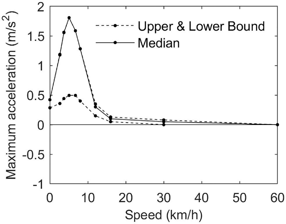
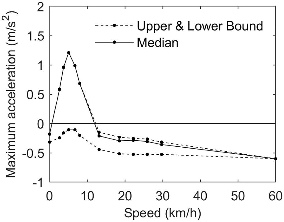
For bicycle traffic, COWI ( 11 ) proposed a maximum-acceleration function (see Figure 1a). Based on this function, the model assigns an individual maximum acceleration value to each cyclist depending on their current speed. Additionally, the distribution among cyclists is specified by three subfunctions: one for the median cyclist (the solid line), one for the zeroth percentile (lower bound dashed line), and one for the 100th percentile (upper bound dashed line). The individual function of each cyclist is then assigned a certain percentile by a random draw. Therefore, the model allocates cyclists randomly within these boundaries given their current speed.
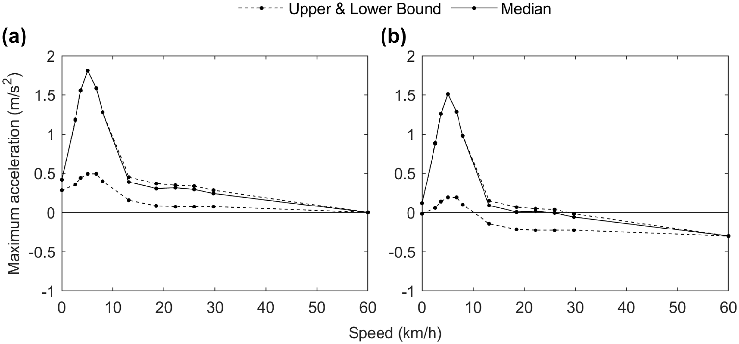
Maximum-acceleration function for cyclists proposed by COWI ( 11 ) on: (a) the flat and (b) a 3% gradient uphill.
For non-flat links, the maximum acceleration is additionally influenced by a gradient-acceleration parameter that reduces or increases the acceleration by 0.1 m/s2 per 1% gradient depending on whether it is an uphill or a downhill ( 25 ), as exemplified in Figure 1b on a link with 3% gradient uphill. This gradient-acceleration parameter is fixed, and the user cannot modify it.
When we consider cyclists assigned to the lower-bound function in Figure 1b, we observe that if cyclists have a desired speed higher than 10 km/h, the maximum acceleration would be assigned a negative value that reduces the speed, while slower cyclists would still have a positive maximum acceleration and should, thereby, be able to reach their desired speed. Using this lower-bound function for maximum acceleration, Figure 2 presents a hypothetical scenario in which four cyclists are initially traveling at different desired speeds (5 km/h, 15 km/h, 25 km/h, and 35 km/h) on a 3% gradient uphill. For cyclists 2, 3, and 4, their corresponding negative acceleration prevents them from continuing to ride at their desired speed. However, cyclist 1 is unaffected by the gradient since the maximum-acceleration function at this speed remains non-negative and the cyclist is already traveling at the desired speed.
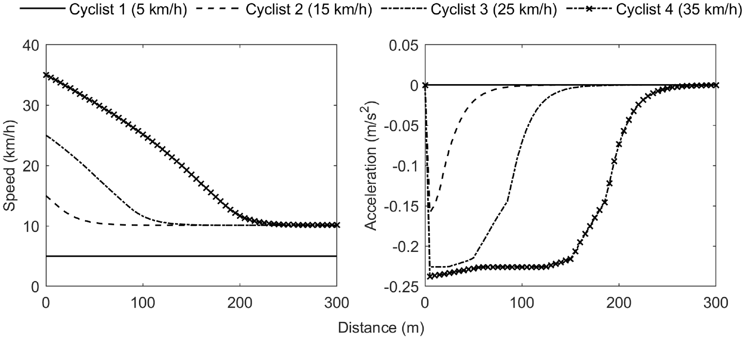
Schematic speed and acceleration profiles of four simulated cyclists traveling at different desired speeds (5 km/h, 15 km/h, 25 km/h, 35 km/h), based on the lower bound of the maximum-acceleration function proposed by COWI ( 11 ) on a 3% gradient uphill.
The simulation of bicycle traffic in Vissim, considering the impact of gradient, has been investigated in a few studies. For instance, COWI ( 11 ) proposed different desired speed distributions to represent bicycle traffic on flat terrains, uphills, and downhills, instead of including the gradient directly in the model. This could be interpreted as if the change in speed resulting from a gradient can be explained mainly by a change in the targeted speed at which cyclists would like to ride, and not by acceleration limitations imposed by the infrastructure. However, it is unclear if the choice of using different desired speed distributions for uphills in COWI ( 11 ) is because of modeling limitations or a belief that this is the most appropriate representation of cyclists’ behavior. Furthermore, the default settings in Vissim might not be ideal to simulate the impact of gradients, according to Henriques and Bento ( 26 ). Instead, the authors introduced external terrain elevation data and custom driver behavior modules to better integrate gradients into the simulation and predict the speed at which a particular selected cyclist would ride on a given uphill or downhill. However, a detailed description of the implemented behavioral model was not presented.
In the above-mentioned studies, the authors demonstrate that a direct connection exists between the gradient and the operating speed of cyclists in Vissim. For unconstrained cyclists, the operating speed depends on their desired speed and ability to ride at the desired speed, that is, the maximum possible acceleration they can apply. In this paper, we investigate the implications of adjusting the gradient-acceleration parameter and the maximum-acceleration function to capture the impact of gradients. Our purpose is to model this impact directly linked to the gradient and the restrictions it imposes on the acceleration, instead of setting different desired speed distributions for different terrain conditions.
Site Description and Data Collection
To carry out the analysis, we use cross-sectional measurements of speed on a bidirectional bicycle path in Munkbron, central Stockholm. The location is far enough away from intersections and under negligible interference from car drivers or pedestrians, making it possible to analyze the speed under conditions only related to cyclists. Near the measurement point, a 30 m stretch, with a longitudinal gradient of 3%, connects the bicycle path alongside a water channel to our measurement point (see Figure 3). The stretch also connects two flat segments of different width: from a section 2.4 m wide alongside the water channel to a section 3 m wide, where our measurements take place.
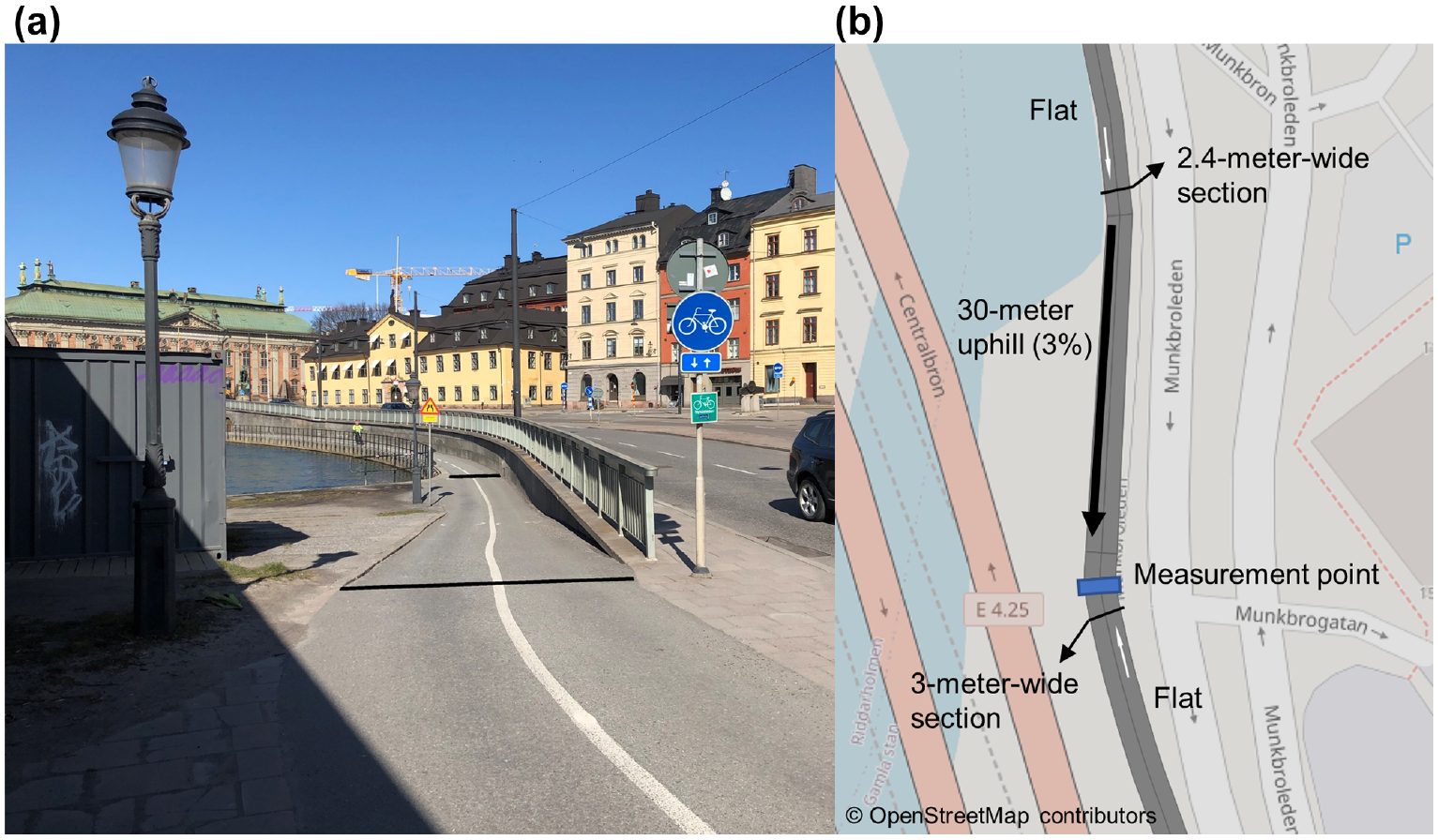
Measurement point at Munkbron: (a) photograph taken at the measurement point and (b) illustration of the 30 m stretch with a 3% gradient uphill that connects two flat segments of different width (from a section 2.4 m wide alongside the water channel to a section 3 m wide).
The data set contains observations of the speed of individual cyclists during 3 days in September of 2018, under good weather conditions. The data were collected in a previous study on estimation of delays in bicycle traffic based on point measurements ( 27 ), which were obtained through automated tracking from real-traffic video data using the Viscando OTUS3D system. Measurement errors caused by the automated tracking and video camera calibration may be present; nonetheless, the investigation of this type of error is outside the scope of this paper. Moreover, we make no differentiation based on individual characteristics (e.g., age, gender, and type of bicycle) so that we meet privacy regulation laws during data collection.
For the purpose of this study, we consider observations during the morning peak period: from 7:00 to 9:00. In total, 9111 speed observations are used (see Table 1). In this paper, we refer to the traveling directions northbound and southbound as the flat and the uphill, respectively. Based on the number of observations, the flows in both traveling directions show a clear asymmetry. The flow, measured in intervals of 15 min, has its maximum peak approximately at 1700 cyclists per hour on the flat, and at 200 cyclists per hour on the uphill. Since many workplaces are located in the city center, that is, to the north of the measurement point, the uneven flow levels between the two directions are reasonable. Additionally, we observed a third bicycle stream coming from and to the adjacent car street near the measurement point. However, this minor stream is deemed to have a negligible effect on the major stream, based on a field visit; thus, it is not considered in the analysis.
Data Summary (Cyclists during Morning Peak Period)
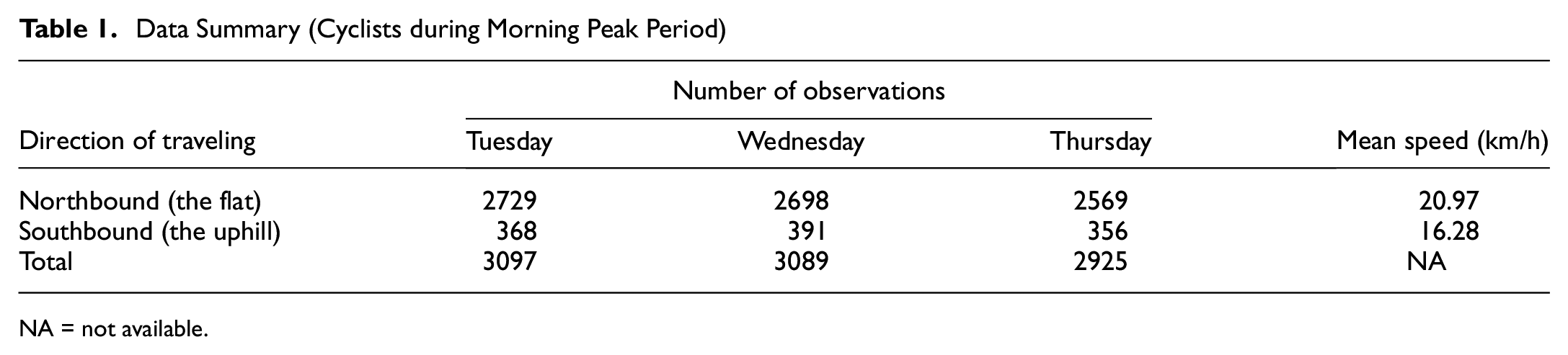
NA = not available.
The observed mean speed also indicates a clear difference between the two traveling directions. Despite the flow being higher on the flat—which could have led to a higher restriction on speed—the speed is higher for cyclists traveling on the flat (20.97 km/h) than on the uphill (16.28 km/h). Given that our measurements take place at the top of the slope, we observe the speed when southbound cyclists reach the top of the slope and when northbound cyclists begin to descend the slope. This non-flat stretch is likely the main cause of the asymmetry between speeds in the two traveling directions; thus, we use this site as a case for the purpose of this paper.
Implementation of the Model
Using the 2020 version of Vissim ( 25 ), we build a model that represents approximately 1 km of the bicycle path, 500 m before and after the measurement point. The demand in the simulation is set to vary according to the measured flow: each 15 min interval of the peak period is assigned a constant demand equal to the corresponding 15 min interval of the measured flow (averaged over the 3 days of data collection). The adjacent links to the gradient are modeled as flat terrain which results in a simulated topography deviating insignificantly from reality.
We use the Wiedemann car-following model 99 ( 25 ) to model the behavior of cyclists, and we define all input related to the following, overtaking, and lateral behavior based on a previous study ( 6 ). Moreover, we set the desired speed distribution based on observations on the flat following a methodology described by Johansson ( 27 ); according to the author, this desired speed distribution is likely to be underestimated since the focus was to estimate delays. Finally, we set the maximum-acceleration function according to COWI ( 11 ) (see Figure 1a) since available references in the literature are limited. Once we build the model, we investigate the following approaches:
Approach A: Changing the gradient. Since the gradient-acceleration parameter (i.e., ±0.1 m/s2 per 1% gradient) cannot be modified in Vissim, we simulate different scenarios varying the gradient to reflect adjustments of this parameter. The idea is to cause a change in the gradient-acceleration parameter by setting the gradient to a fictive value that could represent the 3% real-world gradient (e.g., setting the gradient to 6% would emulate a decrease of 0.2 m/s2 instead of 0.1 m/s2 per 1% gradient). We simulate gradient values between 0 and 10% with steps of 1%, so we simulate 11 scenarios in total.
Approach B: Changing the maximum-acceleration function. In this approach, we calibrate the maximum-acceleration function (see Figure 4). The starting point is the maximum-acceleration function proposed by COWI ( 11 ) and the gradient is set to 3% (corresponding to the real-world gradient). We follow a trial-and-error methodology ( 6 ) to perform the calibration, comparing the simulation output (e.g., speed) to the measurements. The calibration process aims to potentiate the impact of gradient by decreasing all three subfunctions (the median, and the upper and lower bounds), having a greater limitation on acceleration than in the original function.
Combined approach (A+B). Alternatively, we adjust both the gradient and the maximum-acceleration function. In this scenario, we set the gradient to 4% and use the calibrated version of the maximum-acceleration function, also utilized in approach B. The combined approach is intended to limit the drawbacks of both approaches. A description and a discussion of these drawbacks are presented in the results section.
For each of these scenarios, we conduct 20 replications with different random seeds and compare the simulated output to the observed traffic by collecting speed measurements in the model at the same location as the real-world measurement point.
Calibrated maximum-acceleration function.
Results
To get an overview of how sensitive the simulated mean speed is with respect to the gradient, Figure 5 shows the change in mean speed on the uphill as gradient increases. Based on this figure, setting the gradient at the value corresponding to reality (i.e., 3%) would have almost no impact on the mean speed from the simulation. Moreover, setting the gradient to twice the real value (representing a gradient-acceleration parameter value of 0.2 m/s2 per 1% gradient) would result in a fairly accurate mean speed estimate.
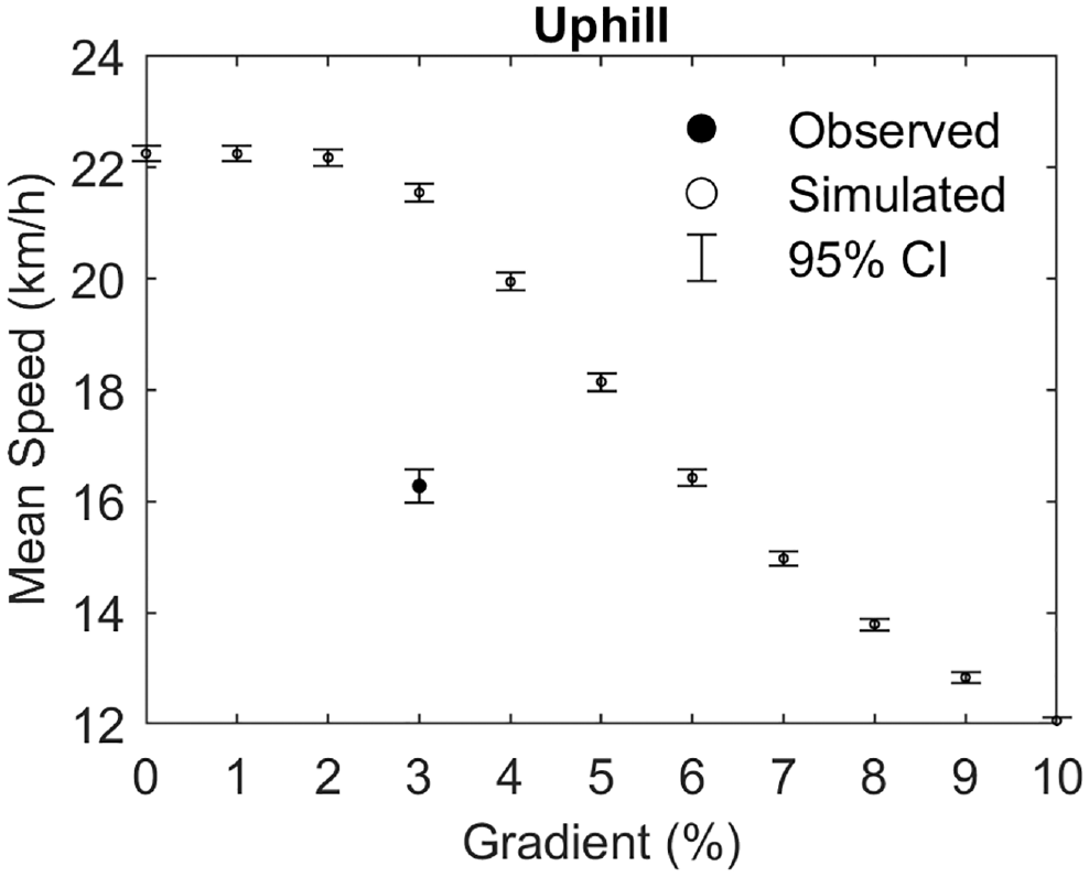
Simulated mean speed versus gradient, and observed mean speed at a 3% gradient.
In respect of effects on the cumulative distributions of speed (see Figure 6), we find that the shapes of the simulated distributions are similar to the observed distributions only for low gradient values. We identify a tendency of less variation in speed among the cyclists at the steepest gradients (see Table 2), and a high asymmetry in the contraction of these distributions at their both extremes. Furthermore, using the real-world gradient would still result in significantly higher speeds than what is observed on the uphill, so a poor estimate of the speed distribution. By doubling the gradient to 6%, most of the estimated speed distribution lies within the 95% confidence interval of the observed speed distributions.
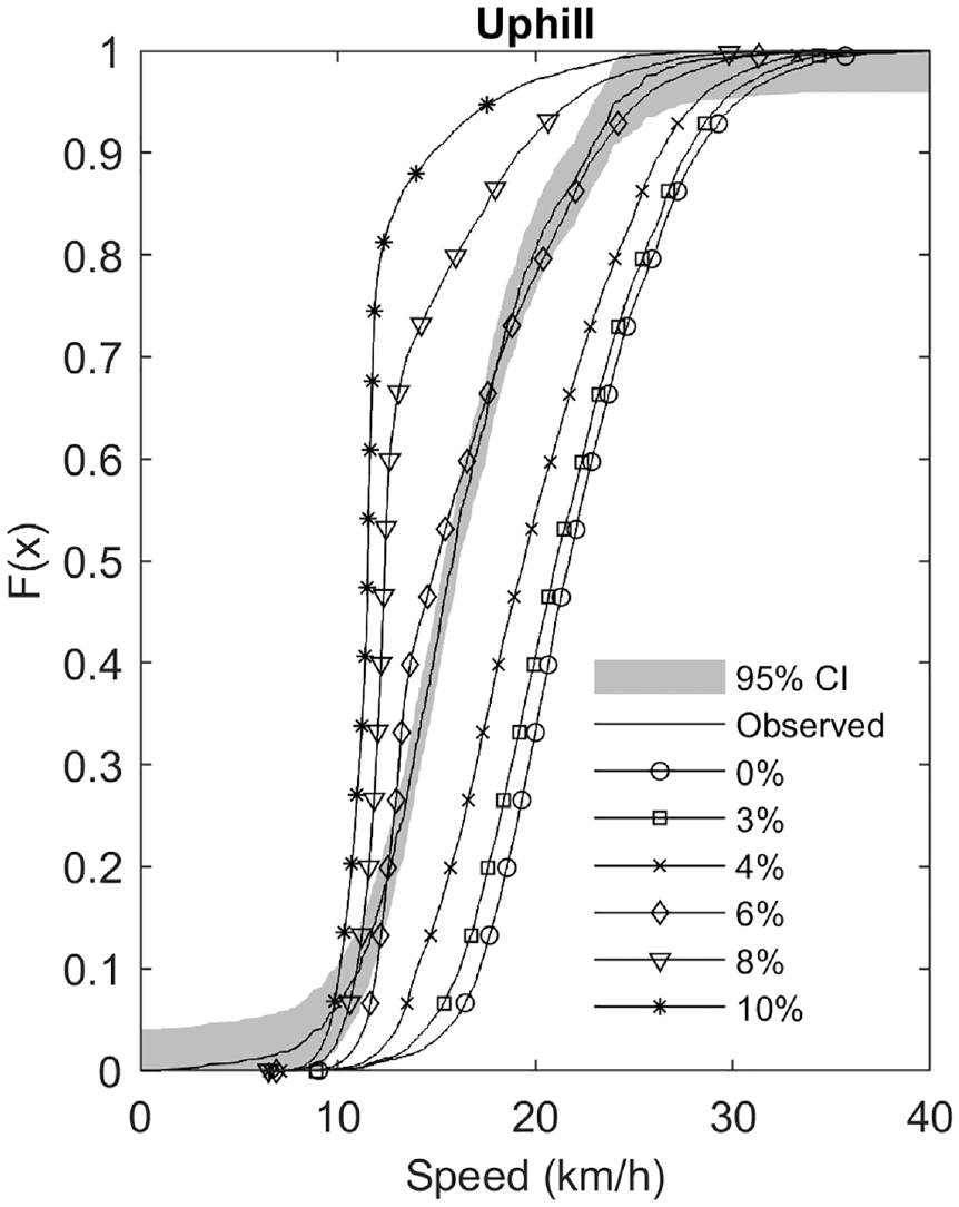
Simulated speed distributions at different gradient values versus observed speed distributions.
Simulated Mean and Variation in Speed between Cyclists at Different Gradient Values, in km/h
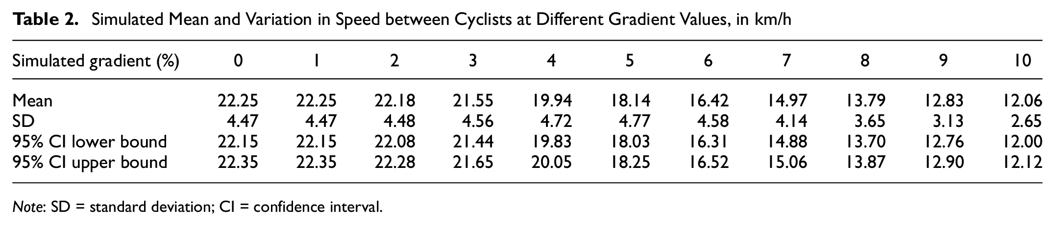
Note: SD = standard deviation; CI = confidence interval.
Figure 7 illustrates the comparison between the simulated and observed speed distributions for each calibration approach; for approach A, we select the 6% gradient scenario as it has been shown to be the best fit (as seen in Figure 6). First, we observe that any of the calibration approaches improves the estimation of the speed distribution on the uphill, compared with the base scenario in which no adjustments are considered for the simulation. However, there are noticeable differences between the approaches.
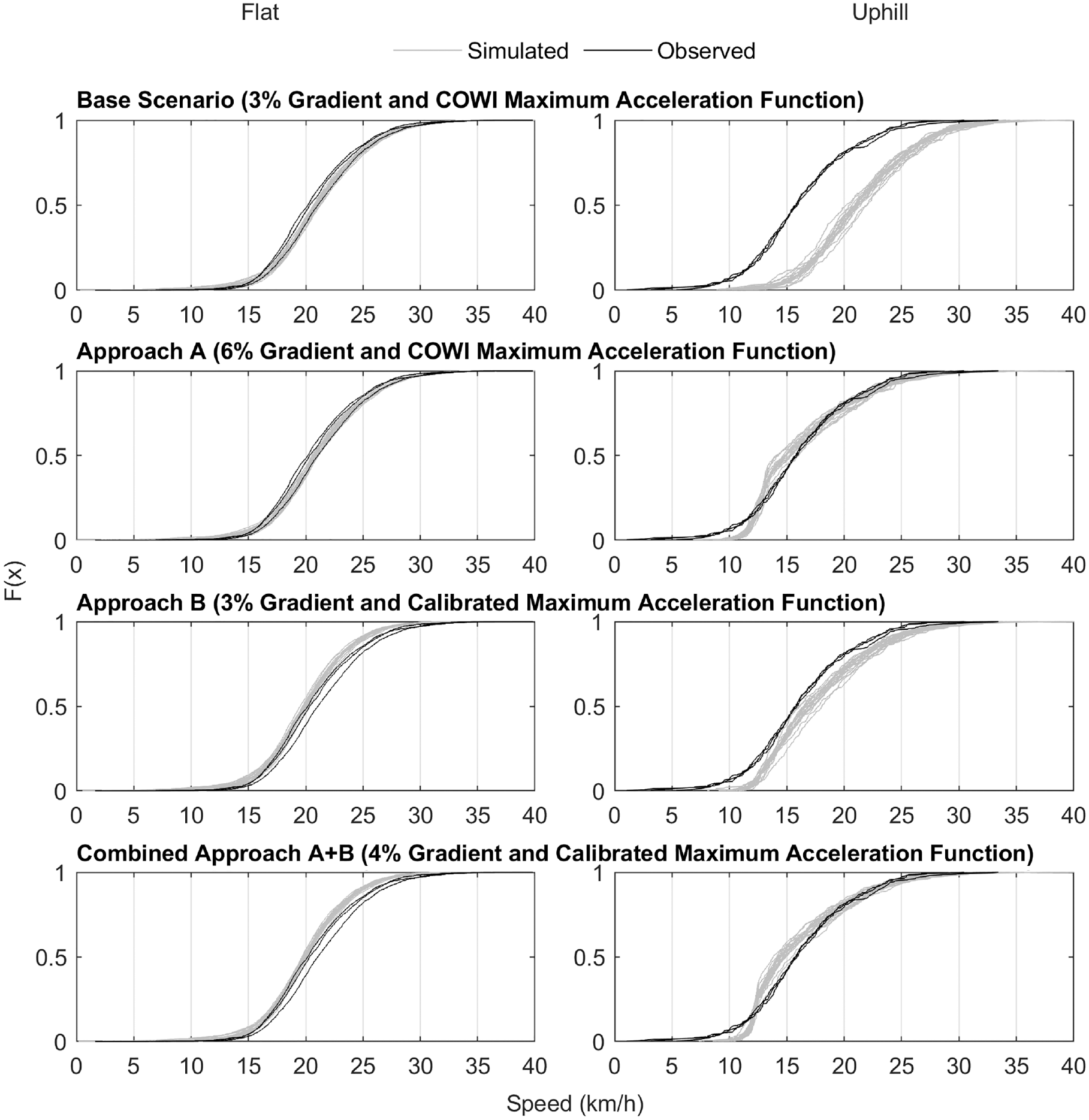
Simulated speed distributions versus observed speed distributions, for both traveling directions.
If approach A is implemented, setting a higher gradient than the real value is necessary to simulate the impact of gradient for cyclists traveling on the uphill, yet the shape of the simulated speed distribution deviates from the observed distribution at certain points. The change in the shape of the simulated speed distribution could be explained by how the maximum-acceleration function is modified in the 6% gradient scenario (see Figure 8). In this scenario (similarly to Figure 2), no cyclists riding at a speed higher than 12 km/h can keep their speed on the uphill and they will all slow down, while for cyclists riding at a speed lower than 12 km/h, at least half of them could accelerate if they desired. As a result, the simulated speed distribution shows an abrupt transition at approximately 12 km/h. Consequently, the gradient may have a very different impact on cyclists depending on their speed and the choice of the upper and lower bounds of the maximum-acceleration function.
Maximum-acceleration function for cyclists on a 6% gradient uphill.
If approach B is applied instead, adjusting the maximum-acceleration function might also bring undesirable side effects for the speed distribution on the flat, that is, for those cyclists arriving at the slope (before descending). By changing the acceleration, we also strongly restrict the opportunities to overtake on the flat, which results in simulating more constrained cyclists who are riding at lower speeds than those observed. The alternative combined approach (A+B) shows no significant improvements for the purpose of this paper.
Finally, we compare the simulated mean speed in each calibration approach to the observed mean speed in both traveling directions (see Figure 9). On the flat, all attempted approaches result in fairly accurate estimations of the mean speed, while on the uphill, only approach A and A+B lies within the 95% confidence interval of the observed mean speed.
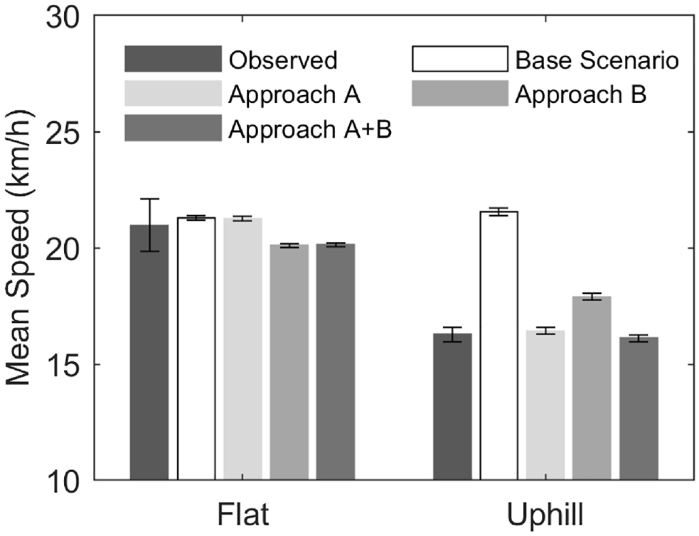
Simulated speed mean versus observed speed mean, for both traveling directions.
Discussion and Conclusions
When using microscopic traffic simulation to evaluate changes in the traffic system, the speed is an important output that needs to be estimated as accurately as possible. In this paper, we investigate one of the factors that influence the speed of cyclists significantly: the longitudinal gradient of a bicycle path. By calibrating either the gradient-acceleration parameter or the maximum-acceleration function, we investigate how the effect of gradient on speed can be captured in the microscopic traffic simulation tool Vissim.
The collected data show a clear difference between the speed in the two traveling directions which is most likely a result of a 3% gradient in the southbound direction. However, simulations of the bike path in Vissim, using the default gradient-acceleration parameter, clearly underestimate the effect of an uphill gradient on the speed of cyclists. Moreover, the reduction in speed variance on uphills, as observed by Ryeng et al. ( 17 ), does not appear until we simulate the steepest gradients. Therefore, if the effect of gradient should be modeled by modifying a maximum-acceleration function, then the gradient should have a higher impact than 0.1 m/s2 per 1% gradient.
Adjusting the maximum-acceleration function by the gradient-acceleration parameter does not directly reduce the speed of all cyclists, but only of those riding above a certain speed. This suggests that for some cyclists, their ability to apply power stays constant over time, so that their desired speed is maintained even for a long uphill (see Figure 2); we consider this situation may not represent the real behavior of cyclists.
A calibrated maximum-acceleration function based on the observed traffic could, in principle, improve the model estimations of speed. However, modifying this function carries some difficulties. First, literature on how the acceleration changes in relation to the speed is limited, particularly for setting upper and lower bounds to this function. Second, the function is also used in the model when cyclists perform overtaking maneuvers or at intersections. Therefore, any changes will also have an impact on the overall traffic performance. In our case, modifying the maximum-acceleration function reduces the acceleration capabilities to overtake in both directions, resulting in a clear impact on the flat; that is, simulated cyclists become more constrained than before which results in lower speeds than those observed. Third, modifying the function affects the complex relation between different factors such as the current speed, the desired speed, and the gradient-acceleration parameter. Considering these issues, defining a maximum-acceleration function such that it accurately represents bicycle traffic performance becomes complex.
We conclude that the Vissim model can reproduce the observed mean speed and speed distributions of bicycle traffic on flat paths. However, for a 3% gradient uphill, neither of the investigated calibration approaches provides accurate estimates of the speed distributions; nonetheless, adjusting the gradient-acceleration parameter by simulating a higher gradient than the real one (approach A) leads to better estimates of the speed distributions than modifying the maximum-acceleration function (approach B). Moreover, approach A fairly captures the observed mean speed on the uphill as opposed to approach B. Among the calibration approaches investigated in this paper, we expect that applying approach A in other locations with different uphill gradients would carry fewer drawbacks than applying approach B. However, a downside is that it requires the modeler to use a different gradient value than the real one.
In this paper, we investigate an application of a car-based modeling approach to bicycle traffic at a specific location. As a result, we demonstrate the limitations of applying a car-based modeling approach to capture the behavior of cyclists on an uphill, indicating the need for further model development. Even though we make some simplifications in the modeling of the selected site, for example in relation to the curvature of the path and the exclusion of a third bicycle flow stream coming in and out of the bicycle path, these simplifications are deemed not to affect the general conclusions since their effect should be small and similar in both traveling directions. However, it is of interest for future research to further investigate the impact of additional elements of the infrastructure at this location, such as the path width narrowing and the presence of barriers on both edges of the bicycle path, that might have some impact on the speed of cyclists, in addition to the gradient.
Although other available traffic simulation software may not use the specific car-based modeling approach investigated in this paper, software often simulates gradient effects in a similar manner, that is, by modifying the maximum acceleration of a vehicle as a function of gradient, particularly focusing on heavy vehicles since they are the motorized vehicle type that is most affected by the slope. Since these modeling approaches are similar to the one investigated in this paper, it is reasonable to expect that car-based modeling approaches, in general, suffer from similar limitations to simulating gradient effects in bicycle traffic.
Compared with car drivers, the physical and behavioral characteristics may vary significantly more among a population of cyclists. Therefore, bicycle traffic is highly heterogeneous in type of bicycle used (e.g., regular bike, e-bike, cargo-bike), cyclists’ characteristics (e.g., age, gender), and cyclists’ preferences for riding. In this paper, we model the heterogeneity of bicycle traffic through a desired speed distribution and a maximum-acceleration function. However, it will be relevant in future research to include heterogeneity at a greater level of detail—for example, considering different types of bicycles or variation in cyclists’ tactical choices to cope with an uphill.
Further research is needed to investigate modeling approaches which directly relate the power and energy expenditure of cyclists when riding uphills, making it possible to model power as a function of time. Certain tactical behaviors differentiate cyclists from other road users; thus, they should also be included in the modeling. One example is the willingness to use more energy to maintain the desired speed during an uphill— some cyclists would not mind the extra effort while others might be concerned about physical exhaustion and sweating, accepting a lower speed than desired. Another example is the willingness to use more or less energy depending on the length of an uphill—for example, if the uphill is short, some cyclists might tolerate increasing power for a short period to overcome the uphill. Finally, additional safety-related concerns might also be involved when riding downhill, as cyclists tend to avoid reaching extremely high speeds.
The gradient is a property of the infrastructure that has a strong impact on the speed and acceleration of cyclists; the speed on an uphill is significantly different from the speed at a flat section. This alone is reason enough to motivate proper inclusion of gradient effects in traffic models, but we also expect that cyclists employ differing riding tactics depending on the slope of the path, which further motivates detailed studies of the effects of gradient on bicycle traffic. Having more detailed knowledge on the speed and acceleration behavior of a population of cyclists in connection with the gradient would allow the investigation of what is the actual effect of gradient on bicycle traffic, and how we can model this effect. To gain more knowledge on the impact of gradients, more locations with different characteristics (e.g., gradient profiles and uphill length) should also be investigated, preferably based on trajectory data which allow for detailed analysis of changes in speed and acceleration. In this paper, by applying a car-based modeling approach to bicycle traffic and thereby demonstrating its limitations to capture the behavior of cyclists on an uphill, we indicate the need for investigating other promising modeling approaches to model cyclist behavior in connection with cycling infrastructure.
Footnotes
Author Contributions
The authors confirm contribution to the paper as follows: study conception and design: G. Pérez Castro, F. Johansson, J. Olstam; data collection: F. Johansson; analysis and interpretation of results: G. Pérez Castro, F. Johansson, J. Olstam; draft manuscript preparation: G. Pérez Castro. All authors reviewed the results and approved the final version of the manuscript.
Declaration of Conflicting Interests
The author(s) declared no potential conflicts of interest with respect to the research, authorship, and/or publication of this article.
Funding
The author(s) disclosed receipt of the following financial support for the research, authorship, and/or publication of this article: This work is funded by the Swedish Transport Administration (Trafikverket) via Centre for Traffic Research (CTR) under grant TRV 2019/84465.
Data Accessibility Statement
Derived data supporting the findings of this study are available from the corresponding author on request. Availability of raw data is limited by contract with Viscando AB.