Sage Journals: Discover world-class research

Abstract

Monitoring environmental features, such as air pollution, carbon dioxide emissions, noise, and heat, gives cities key data-driven insights to advise sustainable policies and city design. However, given the high variability of the environmental data, achieving good spatio-temporal resolution and coverage remains a major challenge. Even in well-monitored cities, such as Amsterdam, environmental sensors are usually placed in very few fixed locations, implying limited spatial coverage and an inability to adapt to changes in the urban environment. As cities evolve, they experience shifts in pollution sources, and fixed sensors might not adequately capture these changes without a costly and time-consuming reconfiguration process. To monitor the environmental qualities of Amsterdam’s roads, we present a “drive-by” sensing solution for a structured network of vehicles, meaning that sensors are designed to be deployed on buses and tramways, the trajectories and schedules of which are known. We propose a deployment strategy that combines the available fleets to reach optimal spatio-temporal coverage for different environmental features. For example, by optimizing the deployment of sensors on public transit vehicles, our proposal significantly enhances the monitoring of pollution-sensitive areas in Amsterdam. Depending on the desired spatio-temporal granularity and noting that one vehicle only hosts one sensor, the required number of sensors to be deployed on the structured network varies between 43 and 142, with the latter achieving the finest possible resolution.

Keywords

sustainability and resilience transportation and sustainability air quality and greenhouse gas mitigation air quality modeling emissions and air quality management

Rapid urbanization across the globe has led to several environmental risk factors in cities, including air pollution, greenhouse gas emissions, noise, and urban heat. Such factors result in various adverse public health outcomes and should duly be regulated. Strong evidence demonstrates that air pollutants, such as particulate matter, carbon monoxide, and nitrogen oxides, can cause acute and chronic respiratory, reproductive, and cardiovascular diseases ( 1 , 2 ). Beyond its effect on auditory health, noise is also commonly found to cause adverse health effects ( 3 , 4 ). Urban heat, a phenomenon gaining increased attention in the context of climate change, is emerging as a significant public health concern, with a much larger geographic scope. Monitoring such environmental features as air pollution, greenhouse gas emissions, noise, and heat gives cities key data-driven insights to advise sustainable policies and city design. However, given the high variability of the environmental data, achieving good spatio-temporal resolution and coverage remains a major challenge. To capture the environmental features of streets, sensors have recently been mounted on vehicles; this allows for the collection of near real-time data over a given geographical area ( 5 , 6 ). This drive-by sensing approach is cost-effective, as it enables the collection of data, for example, on air quality, noise, temperature, and road quality, using already deployed vehicle fleets. It is also highly scalable, with additional sensors being easily deployable, depending on the desired level of coverage ( 7 ).

Previous research has already been focused on optimizing the number of vehicles needed in drive-by sensing strategies. O’Keeffe et al. ( 8 ) explored the use of sensors on taxis to monitor urban environments and found that only 10 taxis cover up to one-third of Manhattan’s street network at least once a day. O’Keeffe et al. ( 8 ) also show that these findings are consistent across different cities, given the taxi fleet over a given road network. Similarly, Anjomshoaa et al. ( 9 ) highlighted the advantages of this drive-by sensing approach, such as lower deployment and maintenance costs, compared with stationary sensor networks. They investigated the effect of street network topology on the quality of data captured through drive-by sensing. Both these studies were investigations of theoretical problems. Practically, there are important spatial biases and temporal limitations. Spatially, as acknowledged by the study authors, taxi trips are concentrated in commercial and tourist areas, leaving large swaths of cities uncovered (symptomatically, the model focuses on Manhattan, rather than New York’s five boroughs)—where socioeconomically deprived populations often reside. Temporally, in these studies, it is not considered that environmental and urban features require different resolutions—for instance, air pollution varies in a matter of seconds, whereas road condition is relatively stable.

This paper presents a practical approach: a drive-by sensing strategy is proposed, based on structured mobility networks (buses and tramways), where vehicles’ paths and timetables are pre-established, allowing for the assignment of sensors to specific bus and tramway vehicles. We acknowledge that taxis’ unstructured network and random motion encompass street segments not covered by structured mobility networks. However, besides the spatial bias and temporal resolution limitation of using taxis, the highest concentration of air and noise pollution (for instance) in a city most probably occurs in areas with high traffic density, where buses and tramways usually operate. In the interest of public health, it is important to monitor these segments continuously. By integrating structured mobility in the sensing network, popular segments are continuously sensed at regular spatio-temporal intervals.

To test the robustness of our model, we focus on one of the environmental aspects that varies the most in space and time, air quality, while including other aspects less sensitive to spatio-temporal variation. We begin by defining the sampling constraints for several parameters (particulate matter [PM], O₃, NO₂, etc.) according to past research. While sampling at regular intervals allows for continuous monitoring in time, the aim in this study is to monitor in both time and space by introducing the sampling frequency as the number of samples obtained along specific locations throughout the network in the study period. We then compute the spatial distribution and schedules of all the public fleets of Amsterdam to eliminate redundancy (near-simultaneous spatial and temporal readings) by discarding overlapping lines as hosts for sensors. This reduces the manufacturing and computational cost of the sensing process. Further analysis is conducted by varying the required number of sensors along the structured network against the sampling frequency, which is the inverse of the location-specific sampling interval. Lastly, we explore further optimization by considering the spatio-temporal sampling requirements for each environmental parameter. The importance of this study lies in its optimized deployment strategy for sensors on structured transportation, offering improved monitoring of pollution-sensitive areas.

Literature Review

In this section, we describe previous findings for measuring (arguably) all the parameters that have been captured by sensors to monitor the live environmental features in urban settings. These parameters are divided into anthropogenic emissions (which consist of air quality parameters and greenhouse gases), tree health, road quality, and noise sensing. Undoubtedly, some of these findings should be referred to as a requirement for efficient monitoring, while the rest serve as a guideline.

Anthropogenic Emissions

Air Quality Parameters

A vast body of literature highlights the significant risks posed by PM to public health, especially among vulnerable populations in densely populated cities ( 10 ). The air quality guidelines (AQGs) established by the World Health Organization (WHO) set various pollutant measurement averaging times, ranging from 1 year to shorter durations, such as 1 h for nitrogen dioxide (NO₂) or 10 min for sulfur dioxide (SO₂). These averaging times (Table 1) are used to assess pollutant concentration levels over specific periods, including shorter- and longer-term exposures throughout the year.

Table 1.

Short- and Long-term Air Quality Guidelines for Particulate Matter, Ozone, Nitrogen Dioxide, Sulfur Dioxide, and Carbon Monoxide ( 11 )

Averaging time	Air quality guideline
PM₁₀ (µg/m³)
Annual	5
24 h^a	15
PM₁₀ (µg/m³)
Annual	15
24 h^a	45
O₃ (µg/m³)
Peak season^b	60
24 h^a	100
NO₂ (µg/m³)
Annual	10
24 h^a	25
1 h	200
SO₂ (µg/m³)
24 h^a	40
10 min	500
CO (µg/m³)
24 h	4
8 h^a	10
1 h	35
15 min	100

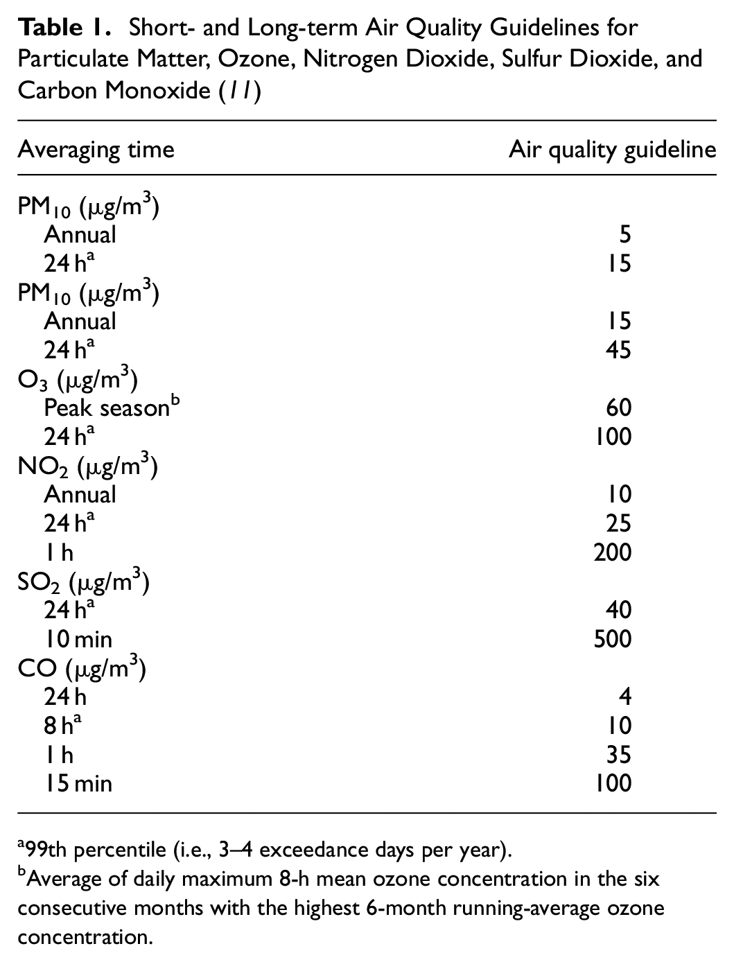
99th percentile (i.e., 3–4 exceedance days per year).

Average of daily maximum 8-h mean ozone concentration in the six consecutive months with the highest 6-month running-average ozone concentration.

To determine compliance with the AQGs listed in Table 1, pollutant measurements need to be made at regular intervals (e.g., every hour) and averaged over a given time frame (e.g., 24 h) to determine the pollutant concentration. Although this provides a general approach to understanding air pollution, it would be more insightful to consider spatial variations within the city. Drive-by sensing becomes relevant here, as it offers broader spatial coverage and finer spatial resolution than fixed stations.

Indeed, street levels of air pollutants can undergo significant changes within a few hours, along with atmospheric transport and dilution processes affected by various meteorological factors ( 12 ). Sampling with a high time resolution provides a more comprehensive understanding of the temporal patterns of pollution concentrations in specific road segments, which can also help to identify specific pollution sources ( 13 ). However, high spatio-temporal resolution mapping implies a much higher computational demand and storage costs, owing to much larger datasets.

Between PM_2.5, PM₁₀, O₃, and NO₂, the smallest averaging time set by the WHO is 1 h. Therefore, for better accuracy, it is necessary to take enough measurements at equal intervals to be averaged over a 1-h period. For SO₂, the minimum averaging time is 10 min; for CO, it is 15 min. However, it will later be shown that the frequency of passage for a public vehicle is generally greater, at least during non-peak periods. Averaging is unfortunately not possible and there can only be about one measurement to be recorded at a given location for both SO₂ and CO. Therefore, to acquire sufficient measurements, the sampling interval at one given location may not exceed the interval of passage of a vehicle at that same location.

Greenhouse Gases

Monitoring greenhouse gases (GHGs) in a city is important to identify pollution hotspots and develop effective strategies to mitigate climate change. However, GHGs, such as carbon dioxide (CO₂) and methane (CH₄), are not typically regulated when applying air quality standards based on short-term exposure or specific concentration limits. In a study, the urban monitoring of CO₂ and CH₄ levels using mobile sensors along 94 km of public transit light rail in Salt Lake County, Utah, provided averaged concentrations during 4-h time windows ( 14 ). Indeed, CO₂ and CH₄ levels are often monitored based on long-term exposure and assessed in the context of climate change and global warming rather than immediate health effects.

As it is most insightful to derive a long-term trend for GHGs with high spatial resolution mapping, it is, therefore, enough for this study to consider one measurement per location per hour.

Mobile Monitoring from Previous Studies

Table 2 lists previous mobile sampling parameters, along with their sampling intervals and study areas. The column headed “Sensor sampling interval” gives the sensors’ inherent sampling intervals along the taken paths in time, but not in space. Therefore, the studies referenced in Table 2 are limited as they do not provide information about the sampling frequency of specific points in the network.

Table 2.

Mobile Sampling Resolution and Study Area for Different Air Quality Indicators

Sensor sampling interval (s)	Study area	Reference
PM_2.5
1	Light Rail, Salt Lake County, UT (94 km) Mannerheimintie, Helsinki, Finland (3.8 km)	Mitchell et al. ( 14 ) Pirjola et al. ( 15 )
3	Tram, Karlsruhe, Germany (65 km)	Hagemann et al. ( 5 )
5	Public Transport, Zürich, Switzerland (91.88 km²)	Hasenfratz et al. ( 16 )
6	MiniMetro, Perugia, Italy (3 km)	Castellini et al. ( 17 )
PM₁₀
5	Public Transport, Zürich, Switzerland (91.88 km²)	Hasenfratz et al. ( 16 )
6	Tram, Karlsruhe, Germany (65 km) MiniMetro, Perugia, Italy (3 km)	Hagemann et al. ( 5 ) Castellini et al. ( 17 )
O₃
2	Light Rail, Salt Lake County, UT (94 km)	Mitchell et al. ( 14 )
6	Tram, Karlsruhe, Germany (65 km)	Hagemann et al. ( 5 )
20–60	Public Transport, Zürich, Switzerland (91.88 km²)	Hasenfratz et al. ( 16 )
NO₂
1	Light Rail, Salt Lake County, UT (94 km) Tram, Karlsruhe, Germany (65 km) Mannerheimintie, Helsinki, Finland (3.8 km)	Mitchell et al. ( 14 ) Hagemann et al. ( 5 ) Pirjola et al. ( 15 )
10	Public Transport, Zürich, Switzerland (91.88 km²)	Hasenfratz et al. ( 16 )
SO₂
1	South, West, and Turku Harbour, Helsinki, Finland	Pirjola et al. ( 15 )
10	Island of Montreal, Canada (472.55 km²)	Levy et al. ( 18 )
CO
1	Tram, Karlsruhe, Germany (65 km)	Hagemann et al. ( 5 )
10	Public Transport, Zürich, Switzerland (91.88 km²) Island of Montreal, Canada (472.55 km²)	Hasenfratz et al. ( 16 ) Levy et al. ( 18 )
CH₄
1	Light Rail, Salt Lake County, UT (94 km)	Mitchell et al. ( 14 )
CO₂
1	Tram, Karlsruhe, Germany (65 km)	Hagemann et al. ( 5 )
4	Light Rail, Salt Lake County, UT (94 km)	Mitchell et al. ( 14 )

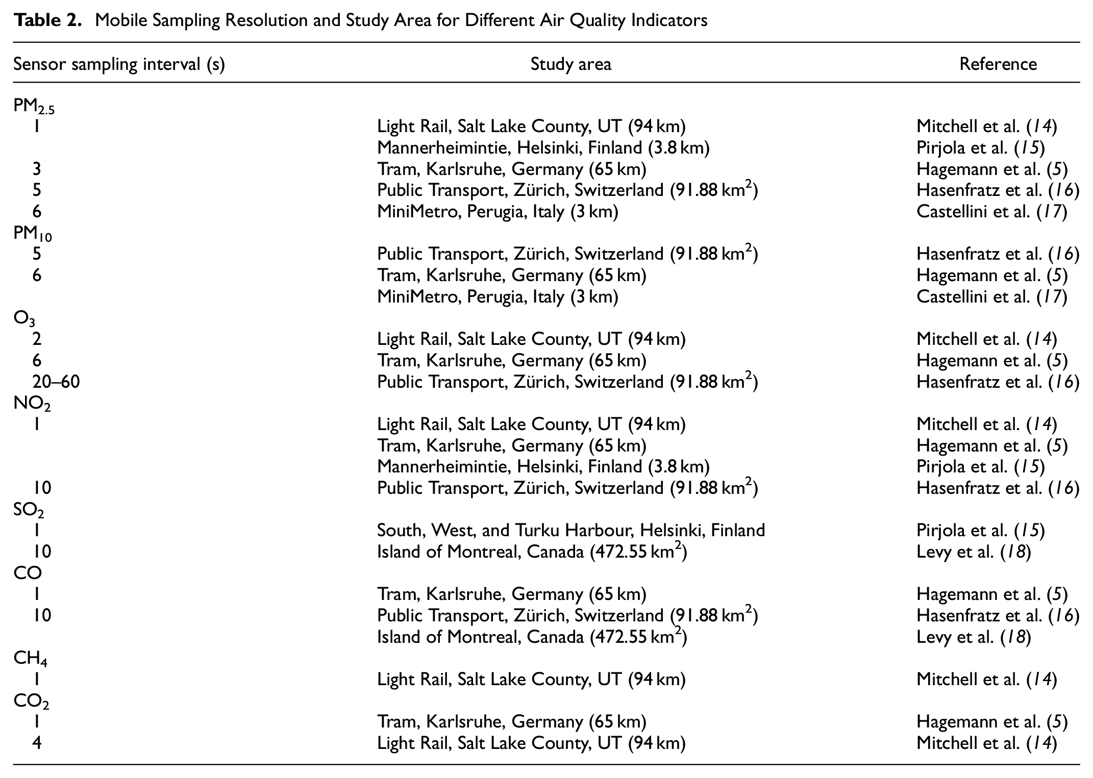
Also, it is important to consider that previous research is built on different network topologies, traffic conditions, sampling methods, and sensor types, and that the spatial resolution changes drastically depending on these conditions. Consequently, although no conclusions should yet be drawn as to the ideal sensor sampling interval for our study, we can infer that it should be of the order of seconds for all anthropogenic pollutants.

Monitoring Tree Health

Another application for monitoring urban environments is mapping the health of trees using infrared thermography, which is a non-contact, non-destructive, and non-invasive technique that enables the detection of radiated heat energy emitted by objects and bodies within the infrared range of the electromagnetic spectrum, typically spanning wavelengths between 0.8 and 14 µm ( 19 ). The conversion of infrared energy into visible imaging is made possible through infrared cameras that produce false-color images.

Sap circulation affects temperature variation along a tree trunk, indicating the health and vitality of functional tissue ( 20 ). Considering that the flow of sap changes between seasons, it is reasonable to set a sampling frequency of one reading per season (every 4 months). However, individual analyses are necessary for a precise health assessment, as different trees with the same pathology may exhibit distinct thermal patterns, owing to varying species, water availability, and temperature gradients.

Road Quality Sensing

Poor road conditions not only lead to vehicle damage but also pose hazards to drivers and pedestrians. Maintaining well-functioning roads is a challenging task, owing to occasional adverse weather conditions, unexpected traffic loads, and natural deterioration that occurs within relatively short timeframes (weeks to months). Given the limited financial resources of municipalities, it becomes crucial to identify and prioritize roads in need of repair.

Solving the problem of road surface monitoring fundamentally requires mobility and cannot be effectively addressed by deploying stationary sensors on roads. Typically, three-axis acceleration sensors and Global Positioning System (GPS) devices are installed on in-car embedded computers, leveraging the inherent mobility of vehicles to traverse and monitor the roads ( 7 ). Fortunately, since road deterioration occurs over extended periods, sampling the road surface daily, or even less frequently, is sufficient ( 21 ). More specifically, road sensing can be activated after sudden changes in temperature and after extreme events (i.e., freeze–thaw cycles or heavy rain), when roads are more likely to deteriorate. The proposed sampling frequency is, therefore, one measurement per location per month.

Noise Sensing

Noise pollution poses a critical challenge in urban areas by significantly affecting human behavior, overall well-being, productivity, and long-term health. As noise and air pollution always co-localize in a city, past research outlined the grave consequences of long-term noise and air pollution co-exposure on human health ( 1 , 4 , 22 ). Previous research also demonstrated that capturing noise data throughout a city is possible using crowd sensing. For instance, Maisonneuve et al. ( 23 ) developed a live participatory noise sensing solution in Paris, France, with a 1-s sensor sampling interval using mobile phones. Parvan et al. ( 24 ) used a 30-s sensor sampling interval. All cases show that a high spatial and temporal granularity of data points is necessary for capturing the short- and long-term variations of noise ( 7 ). However, these past applications are limited in nature, as a single point in space is not being sensed at repeated time intervals.

To better monitor the long-term co-exposure of noise and pollution on a city’s streets, consistency in time for the noise data is needed, which we aim to provide here. One advantage of our approach, in which both sampling interval and frequency are considered, is that it allows for near-continuous noise monitoring in time and space, storing long-term data that can help identify and localize the highest co-exposures through street segments. Owing to the potential risks of noise and air pollution co-exposure, the sampling frequency must be the same as for air quality indicators, and may not exceed the frequency of passage of a vehicle at one specific location.

Methods

We introduce an initiative that enables regular, real-time monitoring of the urban environment. This project utilizes City Scanner sensors ( 7 ), which are low-cost open-source sensors developed by MIT Senseable City Lab. The sensors are intended to be installed on bus and tramway vehicles, which traverse Amsterdam at regular intervals. Amsterdam’s tramway network consists of 15 lines, which operate between 6 and 12:30 a.m., at intervals of between 5 min and 10 min for all lines. The bus network has 43 lines (32 regular lines and 11 night lines), with intervals mostly ranging between 8 min and 15 min during the day, and between 10 min and 35 min at night.

So far, only a handful of mobile urban observation networks integrated with public transit systems have been deployed, which can generate highly detailed air pollution maps. However, in all of these cases, mobile sensing trades off temporal resolution against spatial resolution. In our model, every location in space throughout the network is sensed at regular and short time intervals.

To conduct the optimization study for the structured network in Amsterdam, comprehensive data for bus and tramway transportation networks were gathered from several reliable sources. To ensure accuracy, the primary sources of data were the General Transit Feed Specification (GTFS) schedule, which provides standardized transit data, and the City of Amsterdam’s official administration, known as Gemeente Amsterdam. Additionally, data from Gemeente Vervoerbedrijf (GVB), the municipal public transport operator responsible for operating the bus and tram services in Amsterdam, were utilized.

Sensor Sampling Resolution

To determine the optimal sampling frequency, we must consider the highest sampling frequency, $f_{traffic}$ , related to the traffic flow dynamics—that is, the time it takes for vehicles to pass a fixed point in space. Once the highest frequency is determined, we can apply the Nyquist–Shannon theorem to determine the minimum sampling frequency required. According to this theorem, the sampling frequency should be at least twice the highest sampling frequency, $f_{traffic}$ ( 25 ). For example, if the highest sampling frequency for PM₁₀ is 1 $Hz$ (i.e., pollution variations occurring at a frequency of once per second), the sampling frequency should be at least 2 × 1 $Hz$ = 2 $Hz$ . In other words, we would need to collect pollution samples at a frequency of at least two samples per second to accurately represent spatio-temporal variations. This theorem applies simultaneously in space and time ( 7 ). Considering the highest possible sampling frequency, $f_{traffic}$ , it is, therefore, necessary to set the desired sampling frequency as $F_{s} = 2 \times f_{traffic}$ to accurately capture the highest frequency $f_{traffic}$ of the data being sampled.

Speed variations of the vehicle can introduce Doppler shifts, leading to frequency shifts of the observed signals. Fortunately, typical vehicle speeds are much lower than the speed of light, which means the resulting frequency shifts are generally insignificant. Considering these limitations, the sensors employed for our study typically sample the environment at 1-s intervals ( 6 ). Therefore, to reduce the volume of data being processed, the sensors are set to sample the environment at intervals ranging from 5–10 s for both bus and tramway networks.

Structured Fleet Optimization

Structured modes of transportation refer to public vehicles following fixed trajectories and schedules. They also generally correspond to streets with the highest traffic density and are thus most prone to public health hazards. We use GTFS data ( 26 ) to construct maps, outlining the tramway lines, daytime bus lines, and night-time bus lines (Figure 1). Each color corresponds to one specific line. Overlaps are not yet visible.

Figure 1.

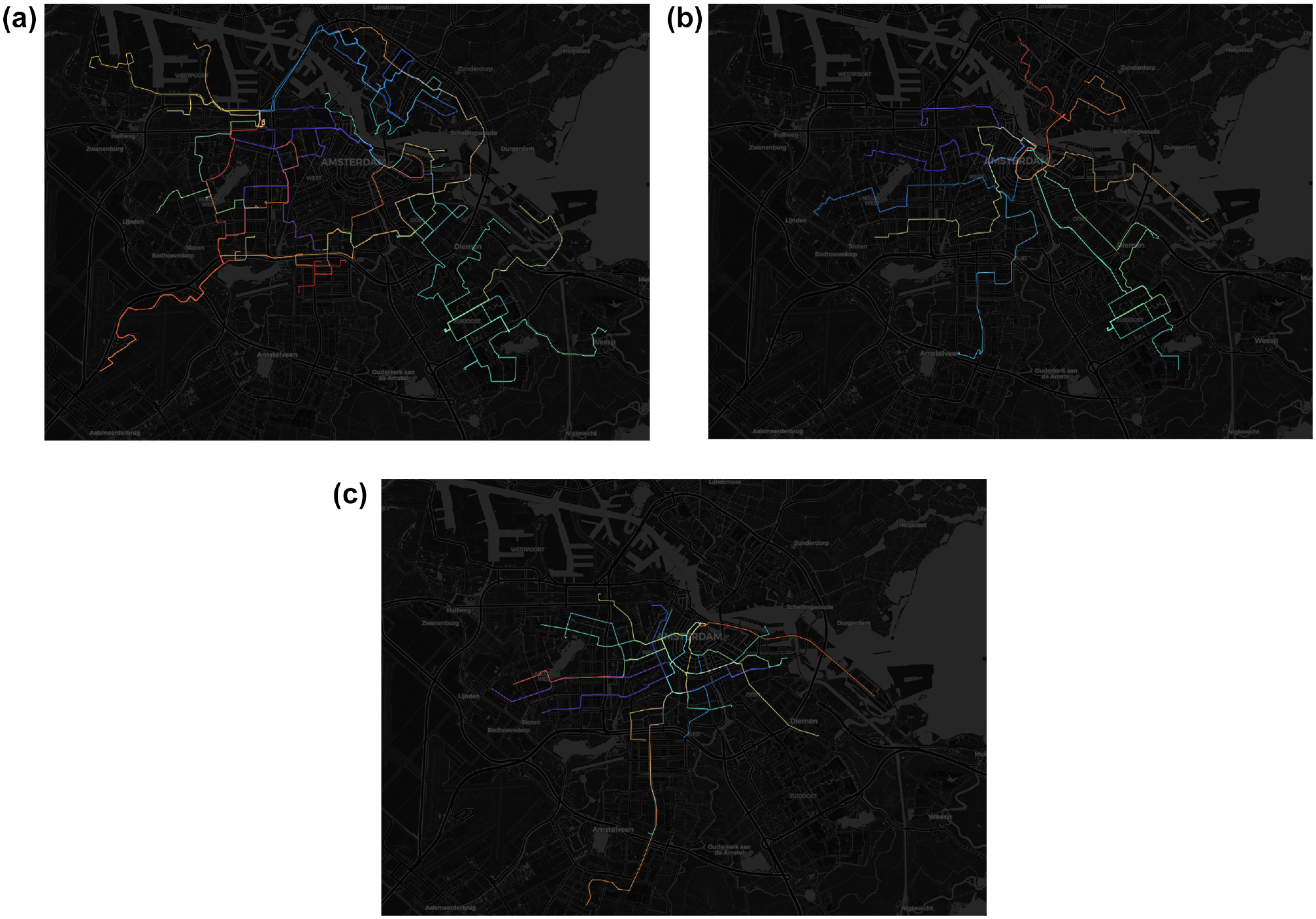
Amsterdam’s (a) daytime bus network; (b) night-time bus network; and (c) day-only tramway network.

Similarity Criterion Approach

To determine which fixed public vehicles will be hosting sensors, the spatial similarity approach considers routing similarity, knowing that schedules are similar throughout the network (mostly between 8 min and 15 min). Considering spatio-temporal granularity constraints, the line with the highest road coverage is the first selected to host sensors. Road coverage is defined by a similarity criterion, $s$ , which is set ahead of the analysis. For example, setting $s = 0.7$ would mean that there is at least 70% similarity in the trajectory of two or more lines. The remaining 30% road segments are classified as under-sampled segments, whose sampling frequency can be improved by the unstructured sensing network. The similarity criterion (described in Figure 2) is simply calculated as

\begin{matrix} s_{traj, k} = \frac{share d_{traj, k}}{traj, k} \end{matrix}

(1)

where, for increment $k$ , $share d_{traj, k} (m)$ corresponds to the trajectory length shared with the longest trajectory, $ma x_{traj, k} (m)$ , and $traj, k (m)$ corresponds to the total length of the considered trajectory.

Figure 2.

Similarity approach flowchart.

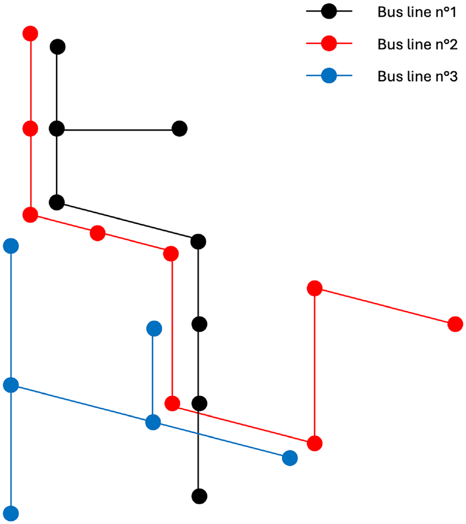
To illustrate the nested loop for the similarity approach, consider the theoretical network in Figure 3. The initial iteration identifies the line covering the longest distance (bus line no. 2) and selects it as the first line to host sensors. Bus line no. 1 shares around 80% of its itinerary with bus line no. 2 $(s_{bus 1, k} > 0.7)$ . Therefore, bus line no. 1 is discarded for hosting the sensors, and the matrix of available trajectories is appended.

Figure 3.

Theoretical bus network.

Then, bus line no. 3 shares around 45% of its itinerary with bus line no. 2 $(s_{bus 3, k} < 0.7)$ . Therefore, bus line no. 3 remains open to receiving sensors, and the matrix of trajectories is not appended. If, during the next iterations, at least one other route is identified with $s_{other, k + 1} > 0.7$ , these other routes will be discarded, and bus line no. 3 will be added to the modes hosting sensors.

Path Discretization and Storage of Overlaps

The similarities in the network are quantified by storing all overlaps between lines. The stored overlaps correspond to shared trajectories. A trajectory is defined as shared whenever two or more different lines run along the same street segment. To identify shared trajectories, the GeoJSON data for all bus and tramway lines are imported into Python and converted to Shapely objects. These objects are then discretized into a succession of equally spaced nodes using linear interpolation, regardless of the total line length, as shown in Figure 4.

Figure 4.

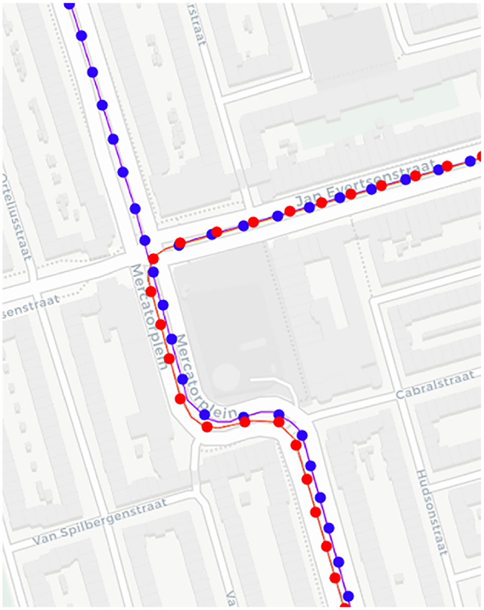
Discretization close-up for Amsterdam’s bus lines 15 and 18.

Another nested for-loop iterates through all nodes for both trajectories and checks whenever the Cartesian distance between two nodes from different trajectories is smaller than a given street width (set as 12 m). Whenever that condition holds true, the concerned nodes are stored, defining all shared trajectories (visualized in Figure 7). Shared trajectories belong to different lines describing the same paths. The next step eliminates redundancy by clustering all similar shared trajectories into one.

Clustering with Symmetrized Segment-Path Distance

Further data cleaning is needed to plot a smooth figure showing the unique shared trajectories (Figure 5). To aggregate similarities from large volumes of raw trajectory data, an advanced approximation method to cluster portions of trajectories with similar shape and length is presented using a shape-based distance first introduced by Besse et al. ( 27 ), the symmetrized segment-path distance (SSPD).

Figure 5.

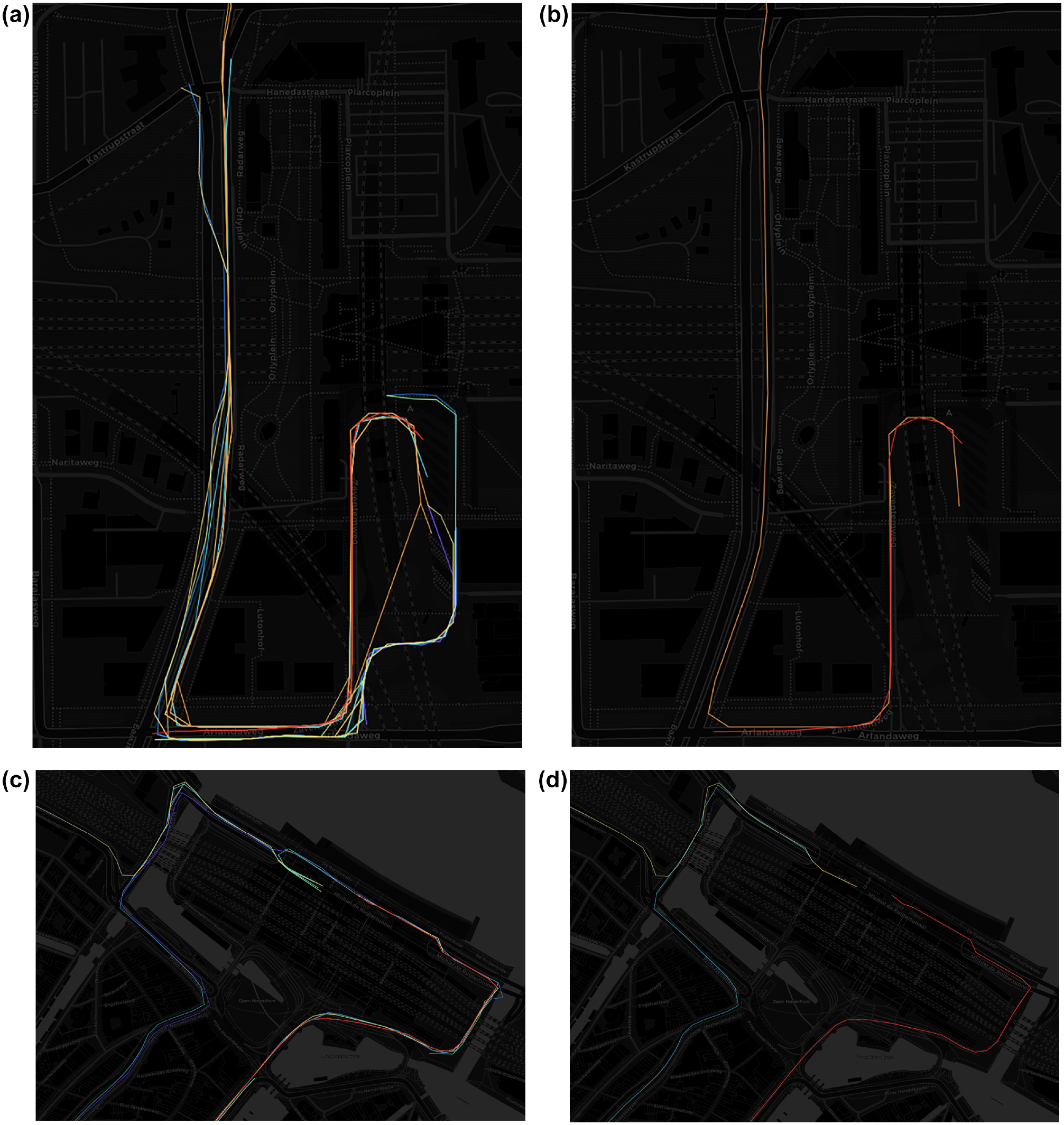
Daytime bus network (a) before and (b) after symmetrized segment-path distance (SSPD). Night-time bus network (c) before and (d) after SSPD.

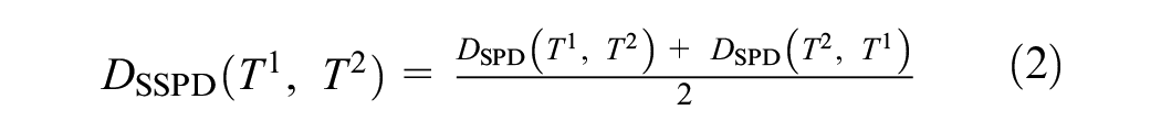
The SSPD is time-insensitive and evaluates both the shape and physical distance between two trajectory objects. We apply this method here because it allows for the comparison of trajectories of different lengths. It also eliminates the need for any additional parameters. Therefore, it can be applied to any set of trajectories, regardless of their geographical origin, resulting in homogeneous clusters. The SSPD is defined by Besse et al. ( 27 ) as

\begin{matrix} D_{SSPD} (T^{1}, T^{2}) = \frac{D_{SPD} (T^{1}, T^{2}) + D_{SPD} (T^{2}, T^{1})}{2} \end{matrix}

(2)

where $D_{SPD}$ defines the asymmetric segment-path distance (SPD) from trajectory $T^{1}$ to trajectory $T^{2}$ and vice versa, meaning that it only considers the similarity in one direction (from $T^{1}$ to $T^{2}$ or from $T^{2}$ to $T^{1}$ ). The SPD (see Figure 6) is defined as the mean of all distances from points composing $T^{1}$ to $T^{2}$ (or $T^{2}$ to $T^{1}$ ):

\begin{matrix} D_{SPD} (T^{1}, T^{2}) = \frac{1}{n_{1}} \sum_{i_{1} = 1}^{n_{1}} D_{pt} (p_{i_{1}}^{1}, T^{2}) \end{matrix}

(3)

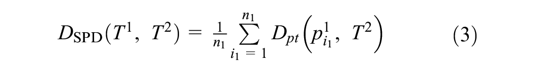
where, considering the minimum distances between point $p$ and segments $s$ that compose $T$ ,

\begin{matrix} D_{pt} (p_{i_{1}}^{1}, T^{2}) = min_{i_{2} \in [0, \dots, n_{2} - 1]} D_{PS} (P_{i_{1}}^{1}, s_{i_{2}}^{2}) \end{matrix}

(4)

Figure 6.

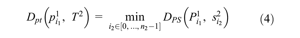
Segment-path distance (SPD) distance: (a) from point $p_{i_{1}}^{1}$ to trajectory $T^{1}$ and (b) from trajectory $T^{1}$ to trajectory $T^{2}$ (28).

Therefore, while the SPD considers similarity unidirectionally, SSPD captures the full similarity by taking the mean of these distances. The final plots after applying the SSPD clustering method are shown in Figure 7.

Figure 7.

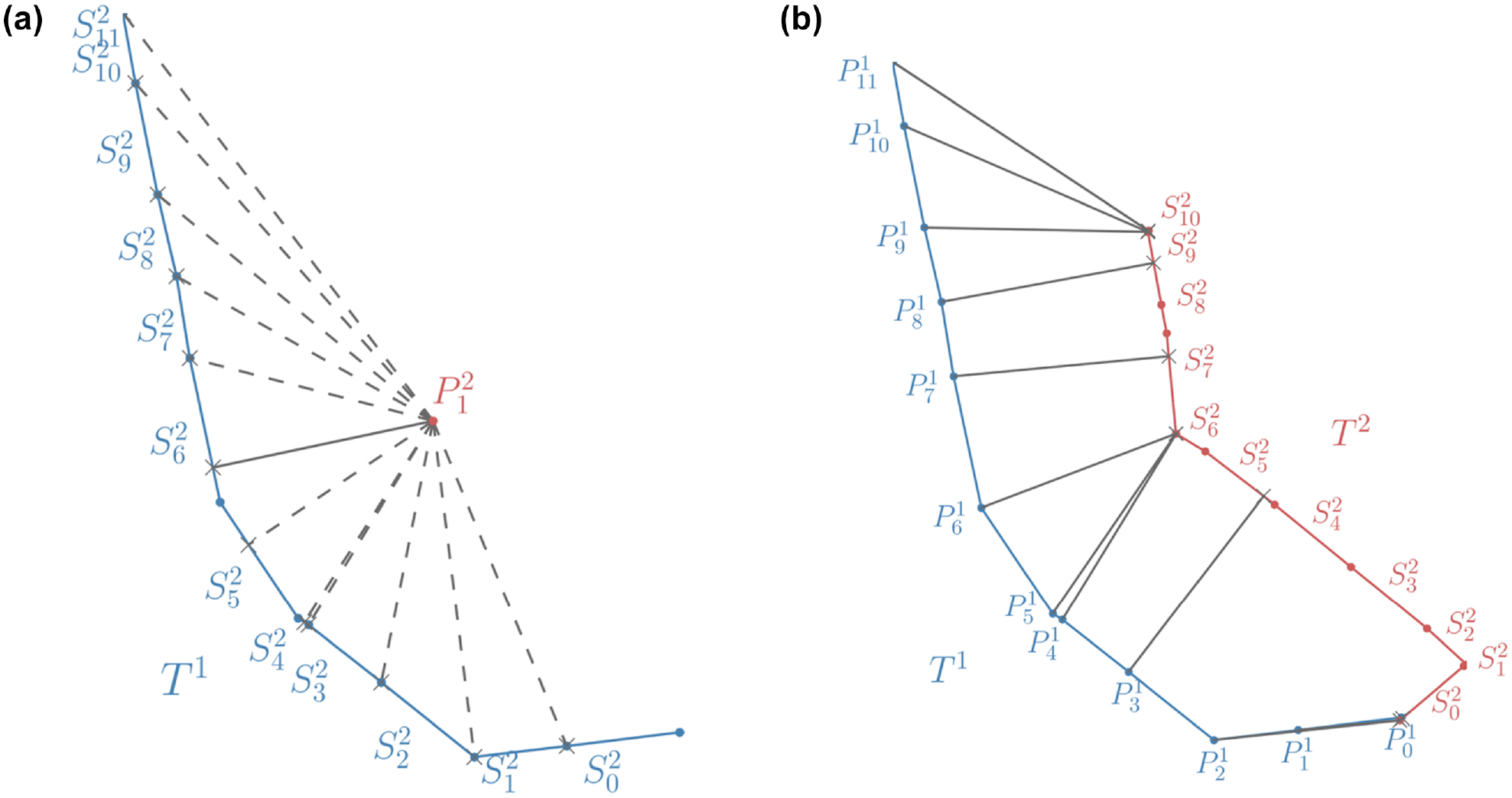
Amsterdam’s overlapping bus line segments: (a) daytime; (b) night-time; and (c) day-only tramway network.

Once the similarity between all lines for both buses and tramways has been computed, it is possible to run an iteration to identify potential lines that could be discarded as sensor hosts as a function of total overlapping. Figure 8 shows the variation in the number of lines to be discarded from hosting sensors when the function of the similarity percentage ranges between 50% and 100%. For instance, setting a minimum similarity tolerance of 60% leads to discarding four tramway lines and eight daytime bus lines.

Figure 8.

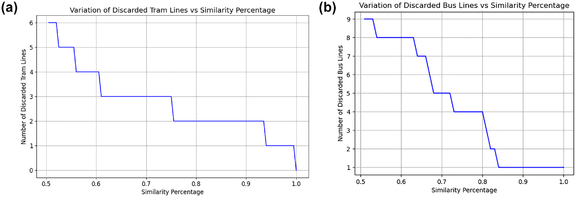
Variation of discarded (a) tram and (b) bus lines versus similarity percentage (day only).

Because there is very little similarity in the bus network during the night (12:30 to 7 a.m.), we do not plot the variation of discarded night-time bus lines with respect to similarity percentage. Since structured networks correspond to the most polluted streets, we decided to discard only lines that shared 100% of their trajectory with other lines (bus line no. 37).

Results and Discussion

As discussed previously, the AQGs for SO₂ and CO showed that the minimum averaging times should be 10 and 15 min, respectively. Therefore, we established that the sampling frequency should be the same as the frequency of passage for tram and bus vehicles, which mostly varies between 6 and 15 min for a given point in space. The number of required sensor-equipped tram and bus vehicles is plotted against the location-specific sampling interval in Figure 9, a and b , and the sampling frequency in Figure 9, c and d , using the available timetables for trams and buses for four different scenarios: morning peak (7 to 9 a.m.), day (9 a.m. to 4 p.m.), afternoon peak (4 to 6 p.m.), and night (6 p.m. to 12:30 a.m.).

Figure 9.

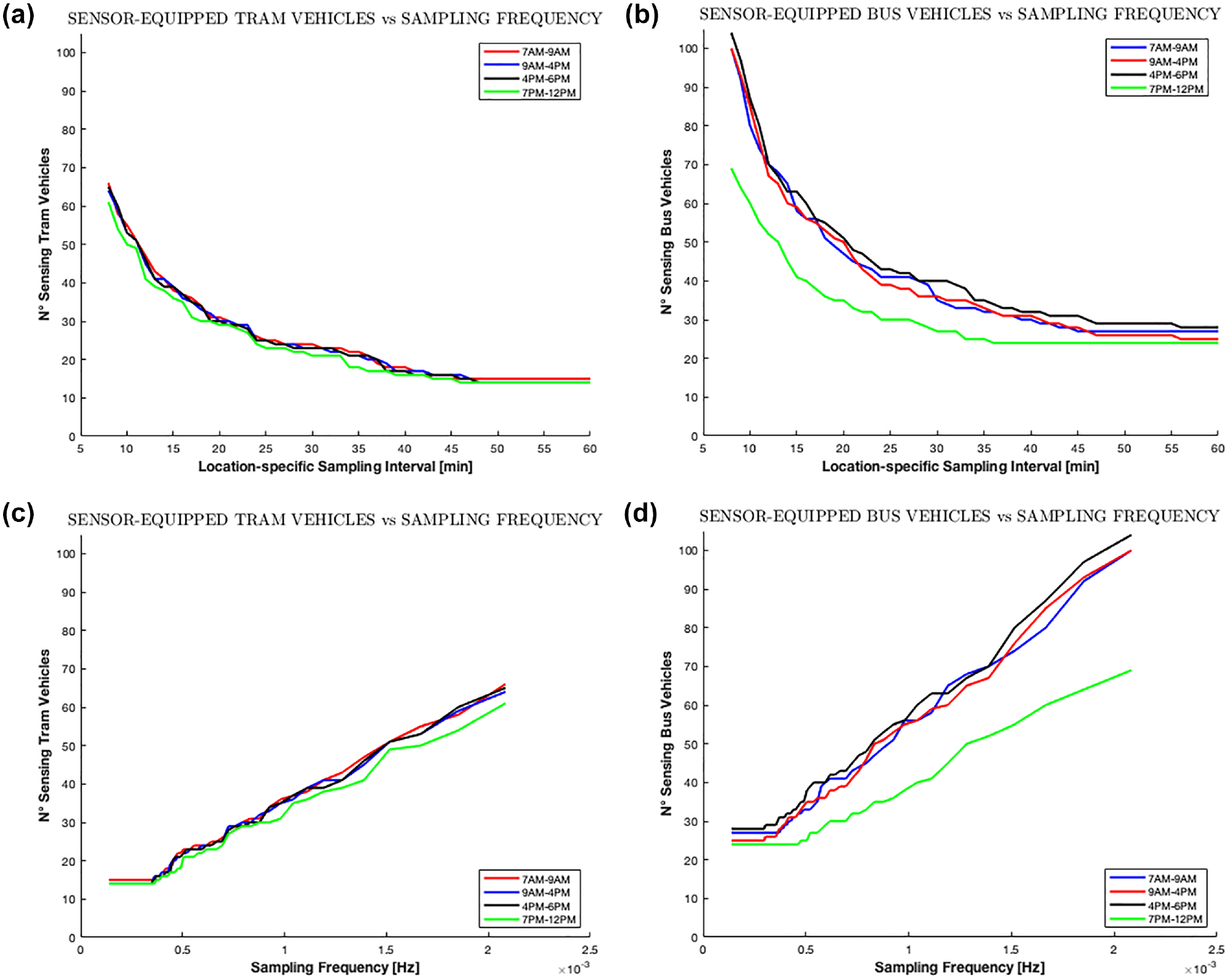
Sensor-equipped (a) tram and (b) bus vehicles versus location-specific sampling interval (daytime). Sensor-equipped (c) tram and (d) bus vehicles versus sampling frequency, continuous coverage scenario.

There is little daily variation in the number of sensors for the tramway plots; tramway lines are not delayed by traffic as they operate on their own road segments. For buses, however, the morning, noon, and afternoon scenarios are similar except for the night scenario. As buses share the road with cars, traffic affects the total trip duration; therefore, more buses need to be dispatched to respect the frequency of passage. The more buses are dispatched, the more scanners are required, which is why the network requires fewer sensor-equipped buses to cover Amsterdam in the evening.

To satisfy WHO’s 10-min averaging time constraints for SO₂ and CO, the number of sensors required would be 55 for trams and 87 for buses (Figure 9). This is for a location-specific sampling interval of 10 min (frequency, $1.67 \times 10^{- 3} Hz$ ). A total of 142 sensors would therefore be needed to continuously cover Amsterdam’s structured transportation network, considering the most conservative scenario. All curves converge to a fixed value at sampling frequencies smaller than $3.47 \times 10^{- 4} Hz$ for trams and $2.98 \times 10^{- 4} Hz$ for buses. Equivalently, they converge for location-specific sampling intervals longer than 48 min for trams and longer than 56 min for buses. For all parameters requiring sampling more often than hourly, the minimum deployable number of sensors is found at the plateaus for both curves (15 sensors for trams plus 28 sensors for buses makes 43 in total).

If only PM_2.5, PM₁₀, O₃, and NO₂ were of interest for the short-term analysis, a 1-h averaging time could imply one measurement every 30 min at one specific location (i.e., two in total to be averaged over a 1-h period). This would also comply with WHO’s guidelines on SO₂ and CO emissions but only for the 1-h averaging case. The total number of scanners would be drastically reduced to around 64 scanners (24 scanners for the tramway network and 40 scanners for the bus network during the day).

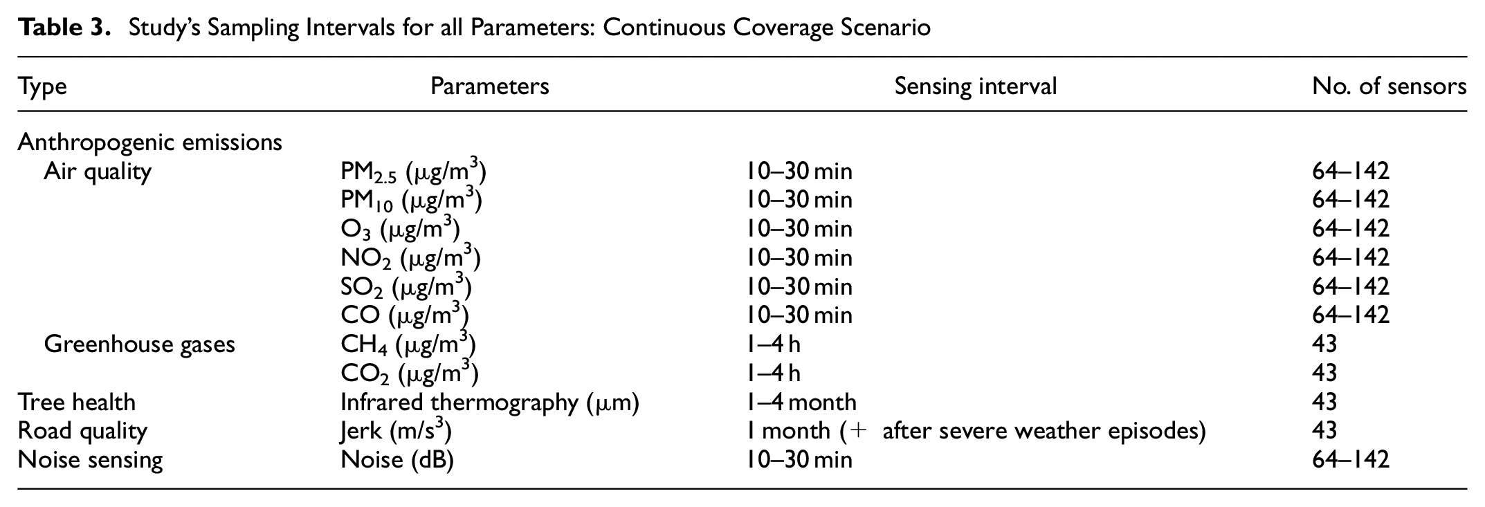
Finally, we can determine the number of required sensors to effectively monitor different parameters in both space and time. Table 3 shows our recommendations for different types of parameter. Overall, the highest number of sensors is needed for air quality and noise sensing parameters. In contrast, GHGs, tree health, and road quality-related parameters require the fewest sensors, namely 43.

Table 3.

Study’s Sampling Intervals for all Parameters: Continuous Coverage Scenario

Type	Parameters	Sensing interval	No. of sensors
Anthropogenic emissions
Air quality	PM_2.5 (µg/m³)	10–30 min	64–142
	PM₁₀ (µg/m³)	10–30 min	64–142
	O₃ (µg/m³)	10–30 min	64–142
	NO₂ (µg/m³)	10–30 min	64–142
	SO₂ (µg/m³)	10–30 min	64–142
	CO (µg/m³)	10–30 min	64–142
Greenhouse gases	CH₄ (µg/m³)	1–4 h	43
Greenhouse gases	CO₂ (µg/m³)	1–4 h	43
Tree health	Infrared thermography (µm)	1–4 month	43
Road quality	Jerk (m/s³)	1 month (+ after severe weather episodes)	43
Noise sensing	Noise (dB)	10–30 min	64–142

Optimizing the sensors’ distribution for structured modes of transportation is straightforward, assuming that the existing network is properly designed in space and that the frequencies of activity for buses and trams fall within the temporal requirements to satisfy accuracy constraints.

But how much does the sampling frequency (and therefore the number of sensors) affect the coverage of the transit network? Figure 10a shows the variation of the total continuously covered distance against the location-specific sampling interval for morning, day, afternoon, and night scenarios. In total, the bus and tramway networks cover a length of approximately 360 km. The curves display a logarithmic growth pattern. The reach increases exponentially at the beginning but at a decreasing rate, indicating that the initial increase in reach is relatively rapid but gradually slows down. The presence of a plateau at a sampling interval of approximately 30 min suggests that, beyond this point, the reach does not significantly increase. The curves level off and reach a point of saturation, indicating that the network becomes fully and continuously covered for larger location-specific sampling intervals exceeding 30 min. The curves display an inflection at a 15-min location-specific sampling interval threshold, meaning that coverage no longer increases rapidly. Therefore, for smaller sampling interval times, sampling has the most effect on reaching broader coverage or achieving a certain level of economic effectiveness.

Figure 10.

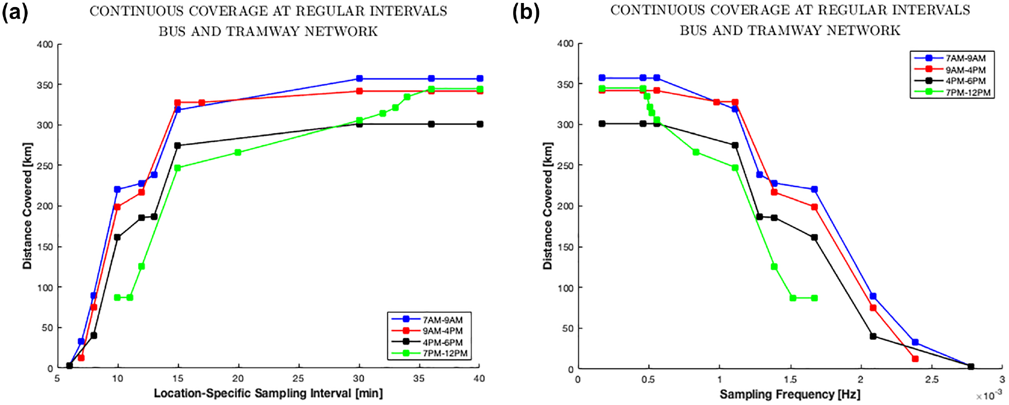
Distance sensed for bus and tramway networks (daytime) continuously in space and time as a function of (a) location-specific sampling interval and (b) sampling frequency.

Although we take Amsterdam as a case study, the power of this research lies in its applicability to other cities. Public transit networks and scheduling are the only required inputs to compute the optimal number of sensors for any given urban area, making this method also adaptable to data-scarce cities in developing countries. Therefore, the presented approach offers good scalability, provided that the spatial and temporal data are complete, regularly updated, and of acceptable quality.

There is also a potential for a hybrid solution integrating both structured and unstructured networks to cover less popular streets using sensor-equipped taxis. O’Keeffe et al. ( 8 ) illustrated the extensive spatial reach of taxi fleets, revealing that only a small number of taxis are sufficient to cover most of a given city spatially, as is consistently observed across various cities considered in their research. However, this also presents certain challenges, given the inherent unpredictability of taxis. Unlike public transit, taxis paths vary, based on customer demands, traffic conditions, and driver choices. This inconsistency in routes and schedules can pose difficulties in ensuring data consistency and optimizing sensing coverage. To mitigate these challenges, a real-time tracking and analysis system could be implemented for the unstructured network. This system would identify streets already covered by the structured network, which is sensed at a very high frequency, and sensors mounted on vehicles with random motion (e.g., taxis) could automatically switch off when passing by the structured network to avoid capturing redundant data. A major advantage would then be energy usage optimization. Because streets covered by the structured network are usually the most popular, the energy life of sensors fitted to taxis would increase significantly. A hybrid structured–unstructured sensing model would, therefore, increase the spatio-temporal reach by encouraging the sensing of remote streets.

Conclusion

In this study, we focused on the practical implementation of a sensing network to monitor the live environmental features of streets in Amsterdam. The drive-by sensing approach, utilizing sensors mounted on public transport vehicles, offers a cost-effective and scalable solution for collecting real-time data on air quality, noise, temperature, and road quality.

The research builds on previous studies that have explored the use of sensors on urban vehicles for environmental monitoring. It extends the scope by incorporating both structured mobility (buses and tramways) and potentially random mobility (taxis) in the sensing network. By integrating structured mobility, the aim is to target areas with high traffic density, where buses and tramways operate, as these areas are likely to have a higher concentration of pollution.

We began the optimization process by defining spatial and temporal monitoring constraints, looking at past research and current regulations set by WHO. We then identified potential lines in the network for sensor deployment. Redundancy was eliminated by discarding overlapping lines to reduce manufacturing and computational costs. We conclude that the required number of sensors varies from 43 sensors for sensing GHGs, tree health, and road quality to between 64 and 142 for the most demanding parameters (PM, O₃, NO₂, etc.), considering the varying sampling frequency for buses and trams.

Overall, this study provides insights into the design and optimization of a sensing network for monitoring environmental parameters in an urban setting. By leveraging existing public fleets and incorporating structured and random mobility, this approach offers a practical and scalable solution for real-time environmental data collection.

Real-time data provide critical insights, which can revolutionize urban planning and policymaking. With precise monitoring of environmental risks, such as air pollution, noise, and temperature fluctuations, Gemeente Amsterdam can more accurately track progress toward its environmental targets. The data serve as a reliable basis for evidence-based and better-informed policymaking, enabling city planners and policymakers to formulate informed decisions based on current, accurate, data rather than on anecdotal evidence or outdated studies. By using the data as a benchmark, Gemeente Amsterdam can set clear and measurable goals for environmental improvement, and regularly review progress.

Moreover, understanding the spatial distribution of these public health risks enables the identification of disproportionately affected communities. This insight supports targeted interventions, ensuring that the most vulnerable populations receive necessary assistance and resources. For example, neighborhoods identified as particularly affected could receive increased funding for green spaces or air quality improvement initiatives. Such targeted measures not only optimize resource allocation, but also promote social equity.

Additionally, making the data publicly accessible in a user-friendly format can heighten community awareness of environmental issues and encourage active participation in sustainable practices. This approach could also foster collaborations between the city, local communities, and researchers, creating a more integrated approach to addressing environmental challenges. Community feedback and involvement can further refine city policies and interventions, leading to a more dynamic and responsive urban sustainability strategy.

Finally, this study is subject to some limitations. While the model presented in this study is practically applicable to Amsterdam, we were not able to control for some factors that can affect the suggested numbers for the sensor deployment, that is, the actual number of transit vehicles dispatched per line and per day, possible switches of service bus lines, and dispatching wait times, especially at terminals. In our future endeavors, we will focus on the hybrid structured–unstructured sensing model, using probabilistic modeling applied to typical assignment algorithms, and addressing the aforementioned limitations.

Footnotes

Acknowledgements

The authors thank Volkswagen Group America, FAE Technology, Samoo Architects & Engineers, GoAigua, DAR Group, RATP, Anas S.p.A., ENEL Foundation, Dover Corporation, AMS Institute, KTH Royal Institute of Technology, and all the members of the MIT Senseable City Lab Consortium for supporting this research.

Author Contributions

The authors confirm contribution to the paper as follows: study conception and design: F. Duarte, C. Ratti; data collection: M. Ariss, F. Duarte; analysis and interpretation of results: M. Ariss, A. Wang, S. Sabouri; draft manuscript preparation: M. Ariss, A. Wang, S. Sabouri, F. Duarte, C. Ratti. All authors reviewed the results and approved the final version of the manuscript.

Declaration of Conflicting Interests

The author(s) declared no potential conflicts of interest with respect to the research, authorship, and/or publication of this article.

Funding

The author(s) received no financial support for the research, authorship, and/or publication of this article.

ORCID iDs

Mayar Ariss

An Wang

Carlo Ratti

References

Cai

Hansell

A. L.

Blangiardo

Burton

P. R.

BioSHaRE de Hoogh

Doiron

, et al. Long-Term Exposure to Road Traffic Noise, Ambient Air Pollution, and Cardiovascular Risk Factors in the HUNT and Lifelines Cohorts. European Heart Journal, Vol. 38, No. 29, 2017, pp. 2290–2296.

Tsai

C. Y.

C. L.

Wang

Y. H.

S. M.

Liu

W. T.

Hsu

W. H.

Majumdar

, et al. Impact of Lifetime Air Pollution Exposure Patterns on the Risk of Chronic Disease. Environmental Research, Vol. 229, 2023, p. 115957.

Smith

R. B.

Beevers

S. D.

Gulliver

Dajnak

Fecht

Blangiardo

Douglass

, et al. Impacts of Air Pollution and Noise on Risk of Preterm Birth and Stillbirth in London. Environment International, Vol. 134, 2020, p. 105290.

Yang

Jin

Wang

Rao

Cai

Y. S.

Huang

Mediation of Metabolic Syndrome in the Association Between Long-Term Co-Exposure to Road Traffic Noise, Air Pollution and Incident Type 2 Diabetes. Ecotoxicology and Environmental Safety, Vol. 258, 2023, p. 114992.

Hagemann

Corsmeier

Kottmeier

Rinke

Wieser

Vogel

Spatial Variability of Particle Number Concentrations and NOx in the Karlsruhe (Germany) Area Obtained with the Mobile Laboratory ‘AERO-TRAM’. Atmospheric Environment, Vol. 94, 2014, pp. 341–352.

Mora

Anjomshoaa

Benson

Duarte

Ratti

Towards Large-scale Drive-by Sensing with Multi-purpose City Scanner Nodes. Proc., 2019 IEEE 5th World Forum on Internet of Things (WF-IoT), Limerick, Ireland, IEEE, New York, 2019, pp. 743–748.

Anjomshoaa

Duarte

Rennings

Matarazzo

T. J.

deSouza

Ratti

City Scanner: Building and Scheduling a Mobile Sensing Platform for Smart City Services. IEEE Internet of Things Journal, Vol. 5, No. 6, 2018, pp. 4567–4579.

O’Keeffe

K. P.

Anjomshoaa

Strogatz

S. H.

Santi

Ratti

Quantifying the Sensing Power of Vehicle Fleets. Proceedings of the National Academy of Sciences, Vol. 116, No. 26, 2019, pp. 12752–12757.

Anjomshoaa

Santi

Duarte

Ratti

Quantifying the Spatio-Temporal Potential of Drive-by Sensing in Smart Cities. Journal of Urban Technology, Vol. 28, No. 1–2, 2021, pp. 199–216.

10.

Han

Chatzidiakou

Yan

Chen

Zhang

Krause

, et al. Difference in Ambient-Personal Exposure to PM2.5 and Its Inflammatory Effect in Local Residents in Urban and Peri-Urban Beijing, China: Results of the AIRLESS Project. Faraday Discuss, Vol. 226, 2021, pp. 569–583.

11.

World Health Organization. WHO Global Air Quality Guidelines: Particulate Matter (PM_2.5 and PM₁₀), Ozone, Nitrogen Dioxide, Sulfur Dioxide and Carbon Monoxide, World Health Organization, Geneva, 2021. https://apps.who.int/iris/handle/10665/345329. Accessed June 12, 2023.

12.

Zhang

Cai

Song

Zhu

The Impacts of the Atmospheric Boundary Layer on Regional Haze in North China. NPJ Climate and Atmospheric Science, Vol. 4, No. 1, 2021, pp. 1–10.

13.

Hodoli

C. G.

Coulon

Mead

M. I.

Source Identification with High-Temporal Resolution Data from Low-Cost Sensors Using Bivariate Polar Plots in Urban Areas of Ghana. Environmental Pollution, Vol. 317, 2023, p. 120448.

14.

Mitchell

L. E.

Crosman

E. T.

Jacques

A. A.

Fasoli

Leclair-Marzolf

Horel J

Bowling

D. R.

Ehleringer

J. R.

Lin

J. C.

Monitoring of Greenhouse Gases and Pollutants Across an Urban Area Using a Light-Rail Public Transit Platform. Atmospheric Environment, Vol. 187, 2018, pp. 9–23.

15.

Pirjola

Lähde

Niemi

J. V.

Kousa

Rönkkö

Karjalainen

Keskinen

Frey

Hillamo

Spatial and Temporal Characterization of Traffic Emissions In Urban Microenvironments With A Mobile Laboratory. Atmospheric Environment, Vol. 63, 2012, pp. 156–167.

16.

Hasenfratz

Saukh

Walser

Hueglin

Fierz

Arn

Beutel

Thiele

Deriving High-Resolution Urban Air Pollution Maps Using Mobile Sensor Nodes. Pervasive and Mobile Computing, Vol. 16, 2015, pp. 268–285.

17.

Castellini

Moroni

Cappelletti

PMetro: Measurement of Urban Aerosols on a Mobile Platform. Measurement, Vol. 49, 2014, pp. 99–106.

18.

Levy

Mihele

Narayan

Hilker

Brook

J. R.

Elucidating Multipollutant Exposure Across a Complex Metropolitan Area by Systematic Deployment of a Mobile Laboratory. Atmospheric Chemistry and Physics, Vol. 14, No. 14, 2014, pp. 7173–7193.

19.

Usamentiaga

Venegas

Guerediaga

Vega

Molleda

Bulnes

F. G.

Infrared Thermography for Temperature Measurement and Non-Destructive Testing. Sensors, Vol. 14, No. 7, 2014, pp. 12305–12348.

20.

Burcham

D. C.

Leong

E. C.

Fong

Y. K.

Passive Infrared Camera Measurements Demonstrate Modest Effect of Mechanically Induced Internal Voids on Dracaena Fragrans Stem Temperature. Urban Forestry & Urban Greening, Vol. 11, No. 2, 2012, pp. 169–178.

21.

Eriksson

Girod

Hull

Newton

Madden

Balakrishnan

The Pothole Patrol: Using a Mobile Sensor Network for Road Surface Monitoring. Proc. 6th International Conference on Mobile Systems, Applications, and Services, Breckenridge, CO, ACM, New York, 2008, pp. 29–39.

22.

Eze

I. C.

Jeong

Schaffner

Rezwan

F. I.

Ghantous

Foraster

Vienneau

, et al. Genome-Wide DNA Methylation in Peripheral Blood and Long-Term Exposure to Source-Specific Transportation Noise and Air Pollution: The SAPALDIA Study. Environmental Health Perspectives, Vol. 128, No. 6, 2020, p. 67003.

23.

Maisonneuve

Stevens

Ochab

Participatory Noise Pollution Monitoring Using Mobile Phones. Information Polity, Vol. 15, No. 1–2, 2010, pp. 51–71.

24.

Parvan

I. C.

Danciu

Balan

Noise Pollution Monitoring Using Mobile Crowd Sensing and SAP Analytics. Proc., 16th International Conference on Engineering of Modern Electric Systems (EMES), Oradea, Romania, IEEE, New York, 2021, pp. 1–4.

25.

Shannon

C. E.

Communication in the Presence of Noise. Proceedings of the IRE, Vol. 37, No. 1, 1949, pp. 10–21.

26.

GVB. Operator Details. https://www.transit.land/operators/o-u173-gvb. Accessed June 12, 2023.

27.

Besse

P. C.

Guillouet

Loubes

J. M.

Royer

Review and Perspective for Distance-Based Clustering of Vehicle Trajectories. IEEE Transactions on Intelligent Transportation Systems, Vol. 17, No. 11, 2016, pp. 3306–3317.

Drive-by Environmental Sensing Strategy to Reach Optimal and Continuous Spatio-Temporal Coverage Using Local Transit Network

Abstract

Keywords

Literature Review

Anthropogenic Emissions

Air Quality Parameters

Greenhouse Gases

Mobile Monitoring from Previous Studies

Monitoring Tree Health

Road Quality Sensing

Noise Sensing

Methods

Sensor Sampling Resolution

Structured Fleet Optimization

Similarity Criterion Approach

Path Discretization and Storage of Overlaps

Clustering with Symmetrized Segment-Path Distance

Results and Discussion

Conclusion

Footnotes

Acknowledgements

Author Contributions

Declaration of Conflicting Interests

Funding

ORCID iDs

References