Sage Journals: Discover world-class research

Abstract

One of the components of a new model, called INTRAMOD, for Indonesia’s domestic freight transport is the logistics model. The logistics model describes shipment size choice and the choice between five different transport chain alternatives involving four main modes: truck, train, vessel, and plane. This paper presents the work to forecast the disaggregate transport chain and shipment size choices for Indonesia’s domestic shipments by applying a deterministic and a stochastic approach. Using a standard economic order quantity model with a consolidation assumption, a deterministic approach is used to determine the transport chain and shipment size, minimizing total logistics cost. As an alternative for this, a stochastic model aims to improve the logistics choice modeling by employing data on the manufacturer’s revealed preferences and stated preferences about only the transport chain choice. The chosen specification for the stochastic approach is utilizing the multinomial logit model. Using the demand elasticities for all alternatives with respect to changes in its transport cost, a comparison will be made between the two approaches. In addition, it is concluded that the deterministic model is susceptible to sticky and flip-flop behaviors. In contrast, this characteristic is absent from the stochastic approach.

Keywords

freight systems freight planning and logistics freight model/modeling

Improving model reliability is an essential component of developing a national freight transport model, and model outputs need to be solidly based on reality to accurately forecast the actions of various actors (e.g., shipper and carriers). The incorporation of logistics operations into the freight modeling framework in the form of a logistics module is one path that has been identified as a potential direction for freight model development ( 1 ). A simplified portrayal of the relation between the choices that freight transport actors make in logistics operations and the causes that lie behind those choices is what is meant by the term “logistics model.” Some important aspects of the logistics model include an analysis of the inventory options and the transport options available on a multimodal transport network ( 2 – 4 ).

According to Abate et al. in 2014, freight transport models that include logistics decisions often rely on optimization theory ( 5 ). In this theory, companies attempt to minimize the annual total logistics cost. These kinds of logistics models can be found in the version of the national freight model that was designed in the first decade of the 21st century for the countries of Norway and Sweden ( 6 , 7 ). The Norwegian and Swedish national freight models were developed within the aggregate–disaggregate–aggregate (ADA) model framework. These models estimate the shipment size and transport chain choices of firms following the economic order quantity (EOQ) concept by trading-off the costs of inventory, order costs, and transport costs to achieve the minimum annual logistics cost. When it comes to the creation of Indonesia’s National Freight Transport Model (INTRAMOD), a strategy very much like this one is taken into consideration.

The INTRAMOD is constructed with three different modules: (1) an aggregate zone-to-zone demand model, (2) a disaggregate logistics model, and (3) an aggregate network assignment model. The first module, the aggregate zone-to-zone demand model, is used to model the zonal trade flow distribution, moving from the production zone to the consumption zone. In the second phase, a first subtask is conducted to disaggregate the zone-to-zone flows into hypothetical firm-to-firm flows. This is done as modeling particular firms’ choices of transport chains (the second subtask) requires this step to be completed before proceeding. After that, aggregation to origin–destination (OD) flows (subtask 3 of phase 2) takes place before conducting network assignment. Having a micromodel by including shipper behavior in the development of a logistics model is intended to bring the model closer to reality, where freight flows depend on many individual decisions. However, an insufficient sample size and the near-absence of data on the freight flows of individual shippers covering an entire nation mean that a fully developed micromodel for all phases is a major challenge. Accordingly, the ADA approach that we use here aims at balancing the model’s plausibility with the limited data that are available for Indonesia’s freight transport system. This paper focuses on the primary logistics model. The deterministic method was utilized in the development of the INTRAMOD logistics model that is in use today (i.e., it follows the EOQ theory). This kind of deterministic model is simple to construct, and the necessary data are readily available; nevertheless, it does not have an empirical foundation because it simply assumes that companies will select the transport network and shipment size combination that has the lowest cost. In contrast to this, a stochastic model (such as a logit discrete choice model) is typically estimated on observed behavioral data. This type of model has the potential to more accurately reflect the actual process of logistics choice decision making ( 8 ), but a disadvantage is that exhaustive disaggregate data collection is necessary. In this context, the purpose of this article is to improve the predictions of the existing INTRAMOD logistics model by taking into account the observed behavior of the manufacturers with regard to their choice of transport chain to enable deeper and more realistic policy analysis.

A transport chain is the sequence of modes used in the process of shipping goods from the point of production P to the consumption location C (PC flows), during which the goods may pass through logistics hubs such as warehouses, distribution centers, and transport terminals ( 1 , 4 , 9 ). According to Huber in 2017, most freight transfers involve more than one dedicated form of transportation ( 4 ). The reason for this is because it is not always possible to move freight directly from the location of production to the location where it will be consumed (e.g., because there is both land and sea in between). In addition to this, direct delivery is frequently not cost-effective (i.e., high transport cost). In light of these concerns, researchers have been placing a greater emphasis on the significant problem of transport chain choice and investigating its possibilities to improve the performance of freight transport models ( 8 , 10 ).

On the topic of transport chain (which is sometimes referred to only as transport mode) choices, there are exhaustive literature evaluations ( 4 , 11 , 12 ). The authors contend that the logistics of the supply chain are quite complicated. Therefore, it is absolutely necessary to identify several significant aspects that play a role in the development of the options for the transport chain. In general, there are three basic considerations that need to be taken into account: First, we need to take into account the players and the complicated dynamics between them. There is potential for many actors to be involved in the organization of the transport chain, each of whom would play a unique function. This results in the formation of complicated interactions, some of which may be interdependent on one another. Second, there is the importance of features of the shipment, such as the dimensions of the shipment (m³), its weight and value, the frequency of the shipments, the amount of time it takes to deliver, and so on. Last but not least come characteristics of the transportation system (e.g., the transportation network and transport terminals).

A relatively small number of national freight transport models are found to accommodate logistics, according to the findings of Huber in 2017, who conducted an analysis of the logistics models present in existing national freight transport models. Only fourteen of the 126 freight transport models that were accessible internationally and that were evaluated involve improvements to multimodal transportation, and almost all of those fourteen freight models were established in industrialized countries ( 4 ). Tuğdemir Kök and Deveci in 2019 conducted an in-depth analysis of previously published freight transport choice models utilizing the stated preference (SP) technique ( 12 ). A more comprehensive review on the topic is covered in De Tremerie in 2018 ( 11 ). This review examines many different aspects, including the transport mode that is being predicted, the most used explanatory variables, the actors that are being studied the most, and the approaches (models) that are being applied the most. Both De Tremerie ( 11 ) and Tuğdemir Kök and Deveci ( 12 ) come to the same conclusion, which is that the cost of transport, the time of transport, the reliability of transport, and the frequency of transport are the most frequently used and powerful variables in explaining the choice of transport mode ( 11 , 12 ). In light of this, the variables and approach utilized in this research were chosen after carefully considering the aforementioned reviews.

Recent years have seen a proliferation of research focused on shifting away from deterministic models and toward stochastic ones ( 1 , 5 , 8 , 13 ). The stochastic technique makes use of the random utility discrete choice model to calculate the chance that a particular combination of shipment size and transport chain will be selected by a shipper. The deterministic model has an inherent flaw that the stochastic approach seeks to circumvent to achieve its goal. The all-or-nothing property that characterizes the deterministic model might have a problem known as “overshooting” or “sticky” decisions ( 13 ). Overshooting happens when the logistics cost function is relatively flat, which means that even small shifts in the cost might result in drastically different options. A “sticky” choice, on the other hand, is made when one alternative is noticeably more cost-effective than the others. Therefore, the improvement of another alternative will not have an influence on this alternative’s mode share unless this alternative ultimately becomes the cheapest option, which then leads to a dramatically different model result. To the best of our understanding, there has been limited focus on studying the selection of transport chains in the context of developing nations within the existing literature on freight transport chain choice. Prior research studies in developing countries primarily focus on improving the logistics performance of specific respondents using disaggregate mode choice data (see Filla [ 14 ]). Other studies often have a limited scope, focusing on urban or regional freight mode choice rather than national applications (see Nugroho [ 15 ]). This paper aims to bridge the gap in the literature on freight transport chain choice in the context of an emerging country, as well as compare the deterministic and stochastic approaches for estimating shippers’ logistics choice, thereby providing valuable insights in modeling the logistics aspect of freight transportation systems.

The following outline introduces the remaining portions of this paper. In the second section, a summary is given of the logistics model within INTRAMOD, covering both the deterministic and stochastic approaches. The datasets that were used are discussed in the next section. In the subsequent two sections, the results of the deterministic model and the stochastic analysis are presented. A cost elasticities comparison between these two outcomes is then offered. Last but not least, the conclusions and suggestions for future work are presented in the final section.

Logistics Model

Deterministic

Within the ADA model system, the logistics model plays a crucial role in defining the logistics decisions by the transport actors, in this case the shipper’s selection of transport chain and shipment size, to transfer the result of the trade model (i.e., PC) flows into mode-specific OD flows ( 16 , 17 ). The optimal shipment size can be derived from inventory theory, which addresses the subject of optimal supply chain management. The calculation of shipment size is directly tied to numerous transport-related decisions, including the selection of the transport chain and the pivotal role played by consolidation of shipments.

The EOQ is a concept created by Ford W. Harris in 1913 to minimize the overall inventory cost and ordering cost within inventory management ( 18 ). In the context of freight transport, this strategy recognizes that the utilization of big-capacity vehicles reduces unit transport costs for large shipments. Nonetheless, large shipment quantities result in increased holding costs because the products must be stocked. The EOQ will therefore identify the optimal shipping size by balancing these two costs. The logistics cost function applied to INTRAMOD for shipping from zone r to zone s with the type of commodity k, shipment size q, and transport chain l is given by Equations 1–6. The total logistics cost ( $G_{rskql}$ ) consists of the order cost ( $O_{kq}$ ), transport cost ( $T_{rskql}$ ), capital cost during transit ( $Y_{rskl}$ ), inventory cost ( $I_{kq}$ ), and capital cost of inventory ( $K_{kq}$ ). The following equations apply cost variables in the total logistics cost in the national freight transport model of Norway, and are also implemented for INTRAMOD.

G_{rskql} = O_{kq} + T_{rskql} + Y_{rskl} + I_{kq} + K_{kq}

(1)

O_{kq} = o_{k} (\frac{Q_{k}}{q_{k}})

(2)

T_{rskql} = c_{rsl} . C . \frac{q_{k}}{C} . \frac{Q_{k}}{q_{k}}

(3)

Y_{rskl} = (i . t_{rsl} . v_{k} . Q_{k}) / 365

(4)

I_{kq} = w_{k} . (q_{k} / 2)

(5)

K_{kq} = i . v_{k} . (q_{k} / 2)

(6)

The variables in the aforementioned formulas are unit order cost ( $o_{k}$ ), annual demand ( $Q_{k}$ ), shipment size ( $q_{k}$ ), discount rate ( $i$ ), transport unit cost ( $c_{rsl}$ ), vehicle capacity ( $C$ ), transport time ( $t_{rsl}$ ), value of goods ( $v_{k}$ ), and unit storage cost ( $w_{k}$ ). Other variables besides shipment size are known. Therefore, the shipment size must be specified before the overall logistics cost can be calculated. The EOQ formula specifies the optimal shipment size as the quantity of purchased product with the lowest total logistics cost, which may be computed by setting the derivative of total logistics cost to zero. From the aforementioned equations, the optimal shipping size is calculated as Equation 7:

q_{k} = \sqrt{\frac{2 . o_{k} . Q_{k}}{(w_{k} + i . v_{k})}}

(7)

The unit order cost for Indonesia includes phone expenses, administrative tasks, and the cost of pen and paper, and is estimated to be £15.72 per order. Based on the typical bank interest rates for business and investment loans, the discount rate is considered to be 10.87%. The storage cost per unit comprises warehousing costs, utility bills, and employee salaries, which are estimated to be 20% of the value of the items.

The shipment size generating module in INTRAMOD first determines the shipment size ( $q_{k}$ ) without considering the transport cost ( $T_{rskql}$ ) by applying the original EOQ function in Equation 1. Because $q_{k}$ cancels out of this equation, the transport cost has no bearing on the optimal shipment size, as shown by Equation 3. In actual situations, however, $\frac{q_{k}}{C}$ (i.e., the number of vehicles) is not equal to shipment frequency ( $\frac{Q_{k}}{q_{k}}$ ). In reality, a partially loaded vehicle will incur the same transportation costs as a fully loaded vehicle. This results in scenarios in which the best shipment size, considering transport costs, may differ from the previous optimization result. Therefore, we employ a comprehensive strategy that takes into account the impact of transport costs on total logistics expenses and optimal shipment size. In this method, the initial $q_{k}$ (rounded to integer values) from Equation 1 is used as a starting point to compute the shipment frequency, which is known as the base frequency. Then, twenty potential shipping frequencies are developed in an effort to reduce total logistics expenses.

Because of the low unit order cost in Indonesia, the original EOQ formulation frequently results in small shipment sizes, therefore increasing shipment frequency. Some frequencies exceed 365 shipments per year, which appears unlikely in practice. As a result, a maximum delivery frequency of 365 shipments per year is imposed as the program’s limitation. After that, the twenty potential frequencies in the range [1 to 20] for base frequency 20 and in the range [0.2 $\frac{Q_{k}}{q_{k}}$ , 1.15 $\frac{Q_{k}}{q_{k}}$ ] for base frequency >20 are determined. Using the twenty potential frequencies for Equation 1, trial computations have been undertaken to determine the total logistics cost with a consolidation assumption. The consolidation assumption refers to the situation in which a carrier combines multiple smaller shipments from various shippers into a single truck load to reduce transport costs.

Stochastic

The multinomial logit (MNL) model, being widely used for such estimation, was then applied as a starting point for running NGene software to obtain the efficient experimental design for a SP experiment. The same type of model is also used for analysis after the SP data have been collected (together with revealed preference [RP] data). Such MNL models have error terms which are distributed independently and identically across alternatives and respondents, following the type I extreme value distribution, which leads to the logit formula ( 19 ). Employing the utility function with a single parameter per attribute and alternative specific constants for each alternative (minus 1 for normalization), the utility of each SP-alternative can be expressed by Equation 8 below. Category (i) is a choice alternative using a specific transport chain type.

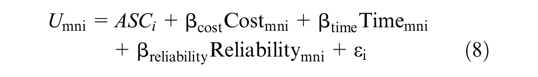
U_{mni} = AS C_{i} + β_{cost} Cos t_{mni} + β_{time} Tim e_{mni} + β_{reliability} Reliabilit y_{mni} + ε_{i}

(8)

where

U _mni = Utility of choosing a discrete transport chain alternative i by shipper q (this index is not shown to reduce complexity) for shipment from m (origin) zone to n (destination) zone

ASC _i = Alternative specific constant for alternative i

β_cost = Parameter of transport cost

Cost_mni = Transport cost of a discrete transport chain alternative i for shipment from m to n

β_time = Parameter of transport time

Time_mni = Transport time of a discrete transport chain alternative i for shipment from m to n

β_reliability = Parameter of reliability

Reliability_mni = Reliability of a discrete transport chain alternative i for shipment from m to n

ε_i = Error term

The values of the transport cost and transport time attributes presented to the respondents are varied around base values which depend on the location of the goods’ origin and destination. As no available data supported these fundamental attributes, a tool to calculate “base value” data on transport cost and transport time between all zones for each type of transport chain alternative was developed, called “the transport chain builder” (TC builder). A brief explanation of the TC builder is provided in the next section. The last attribute is the reliability, which is defined as the percentage value of “how often the shipment is delivered on time.” For example, if a shipper makes five shipments within a month, in a case where a shipment is delayed once a month (not considering the length of the delay), the reliability is 80%.

Moving from Deterministic to Stochastic

There are several reasons for extending the current deterministic model within INTRAMOD to a random utility logistics model (i.e., stochastic). First the behavior of transport actors in a deterministic model is not based on observed data, but on the assumption that shipper will select the transport chain that minimizes costs under certain conditions (from the point of view of the modeler this is dependent on the transport network, the possibility of using transhipment, and the unit transport cost). This assumption is not entirely false, especially for shipments in bulk markets. Second, it is problematic that we do not have access to complete information for all factors that shippers consider when making decisions. Instead of using actual (observed) transport costs, the logistics model assumes that transport costs can be calculated from network information. Therefore, we need a way to account for the lack of actual cost information. Caspersen et al. in 2016 suggested that having the empirical RP data at the level of individual shipments can serve as the foundation for an econometric analysis ( 20 ).

Still according to Caspersen et al., explanatory factors that are not included in the calculated logistics costs may cause problems because the selection of a transport chain could also depend on reliability and mode flexibility ( 20 ). It is difficult to determine the extent to which these factors influence the perceived costs of the shipper. To include, for instance, reliability as a component of the logistics cost, it is necessary to have a meaningful conversion between some metric of measured reliability and monetary units. Here, the RP and SP data have the advantage that they can provide this information directly. The RP data include observed choice information that is the result of all relevant factors, allowing for the estimation of constants per transport chain alternative. Further, the SP data are presumably powerful to estimate coefficients for factors such as reliability of modes. Estimation of a joint model with SP and RP data is widely found in studies on the value of time and value of reliability in freight transport ( 21 – 24 ).

Lastly the main disadvantage of a deterministic model is that the impact of changes in transport policy variables (e.g., a new road, railway, or terminal) can lead to implausibly large responses, or so-called “overshooting” or “flip-flopping” behavior. This occurs when the relevant portion of the logistics cost function is relatively flat, so that a small change in logistics costs can result in a shift to a different optimal shipment size and transport chain. In case of the Norwegian freight transport model, this phenomenon does not always occur and can be mitigated to some extent by employing multiple firm-to-firm (f2f) flows in the model that do not need to move in the same direction ( 20 ). In addition, if the optimal option has significantly lower logistics costs than the second-best option, the model’s behavior could be quite stable (but this could be an exaggeration as well: “sticky” behavior).

In summary, by estimating disaggregate random utility models with available SP and RP data, all of these issues can be resolved. The observed of disaggregate shipment data will then serve as the empirical basis for the model’s behavioral coefficients. These are probabilistic models by definition, as they incorporate a stochastic component to account for the impact of omitted factors. Effectively, a deterministic model assumes that the stochastic component can be ignored, that is, that the researcher has complete knowledge of all the drivers of behavior and that there is no randomness in actual behavior. As a result of adding the stochastic component from random utility modeling, the response functions (now expressed as probabilities) become smooth, as opposed to being aggregated between 0 and 1 in a deterministic model.

Data Analysis

We begin this section by introducing the main module of the intermodal transportation network within INTRAMOD, which we will denote as the TC builder, to generate the explanatory values for the variables of the deterministic logistics model (i.e., transport cost and transport time). The TC builder model portrays the interaction between transportation network and possible transport chain combinations and the level of service connecting origin and destination location. In the TC builder, a node could represent a TC zone (i.e., the centroid of a group of subdistrict areas), a transport terminal, and a road junction. The link acts as a connector between nodes that depict the roads, railways, sea routes, and flight routes. The transport chain’s determination follows the Dijkstra shortest path algorithm based on the minimum total transport cost. From this path, then the total transport length and transport time will be calculated. Apart from the unit transport cost per kilometers and speed variable, the total transport cost and total transport time also consider the handling cost and waiting time at the mode interchange location (i.e., railway station/terminal).

On the other hand, the data for the stochastic approach use both the TC builder result and the online RP/SP survey. There are three parts in the online survey, the first part being an inquiry about the respondent’s company details. In the second part, there are three sections related to the shipment: (1) type of commodity, (2) details of the current choices of shipment transport chain and shipment size (RP data), and (3) the SP scenarios. The third part is a question related to the effect of the pandemic on their shipment choices. Both the RP shipment data and the SP responses will be considered in this paper. For this main survey, 3,374 potential respondents were invited. This resulted in 178 respondents who completed the questionnaire partly or fully, with an average response rate of 5.5%. From those respondents, 236 responses were obtained relating to the commodity type and the OD pair of the shipment, and 179 responses for the valid RP of transport chain and shipment size (i.e., RP shipment). The response is higher than the number of respondents as the possibility of multiple shipments per respondents was offered. Meanwhile, with regard to the SP choices, 624 valid choice observations were gathered to be input for the stochastic approach.

The breakdown of respondents according to Indonesia’s five largest islands is as follows: Java 116 respondents (65%), Sumatra twenty-eight (16%), and Sulawesi fifteen (8%), with Bali and Kalimantan having the lowest share of about 5% each with ten and nine respondents, respectively. The distribution of participants based on the main islands is considerably uneven, with the western islands (Java and Sumatera) having the highest portion. Nevertheless, there are a few participants that are representing the eastern region of Indonesia. Meanwhile, based on the type of commodity group according to first-digit standard goods classification transport statistics (NST/R numbers 0 to 9), the highest number of respondents are the shipper of NSTR 9 (101 respondents), followed by NSTR 0/1 (ninety-six respondents), NSTR 7/8 (twenty-three respondents), and NSTR 6 (six respondents). The least respondents are from NSTR 2/3 and NSTR 5 (five respondents), whereas there was no respondent at all for NSTR 4. Because of the absence of participants for NSTR 4, it is not possible to execute the calibration of the logistics model for this specific NSTR type. As for the purposes of model development of other modules (beyond the logistics model), this NSTR 4 (ores and metal waste) will be assumed to have characteristics close to NSTR 5 (metal products).

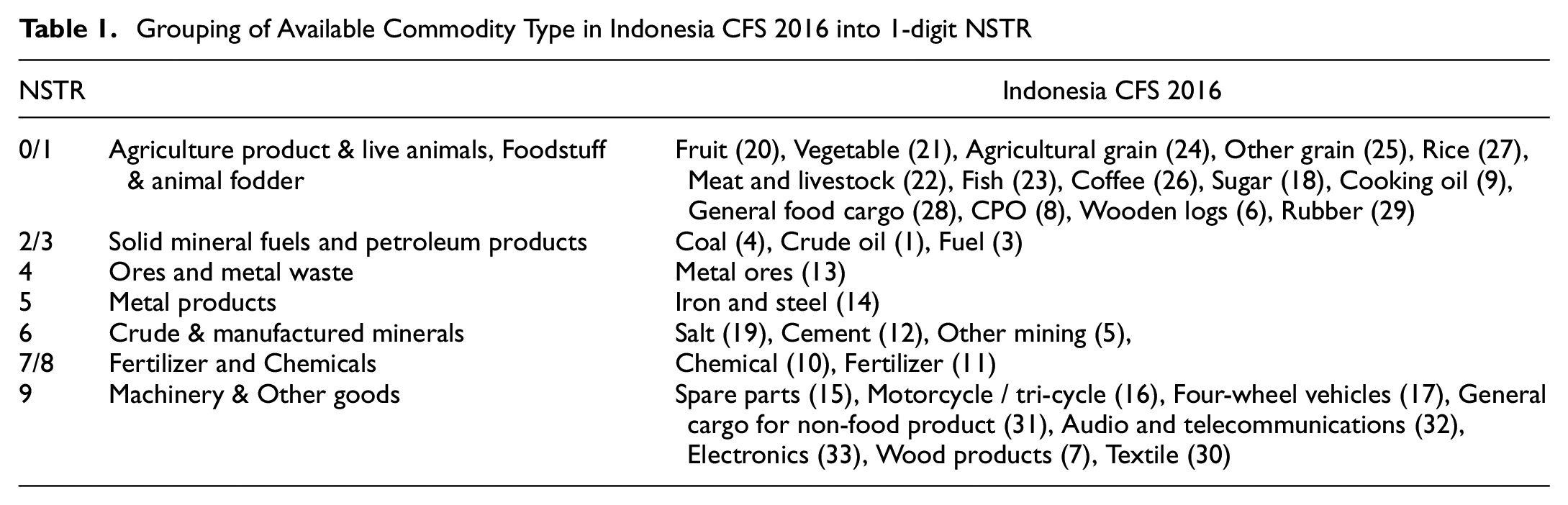
In addition, data related to freight flows were obtained from the Commodity Flow Survey (CFS) carried out by the Ministry of Transportation in 2016. There are thirty-three commodity types, as provided in Table 1. These commodities then will be simplified into 1-digit of NSTR. The CFS data available are at the aggregate level, or the flows between provinces. These data may have some faults, such as not covering some regions, and there are some missing data. However, these data form the most up-to-date dataset we could obtain at the moment, classified by type of commodity, as the previous CFS data were gathered in 2011, which may no longer be relevant. There could be major changes in flows and in the transport network as it was obtained more than a decade ago, and it is not classified by type of commodity. In other words, these CFS data are the best alternative we have at hand. However, as we have no detailed information in regard to the analysis process of these data, their reliability to some degree remains unclear. Table 1 displays the grouping of available commodity types into 1-digit NSTRs. In the meantime, the Indonesian statistics provide information about the number and type of establishments.

Table 1.

Grouping of Available Commodity Type in Indonesia CFS 2016 into 1-digit NSTR

NSTR		Indonesia CFS 2016
0/1	Agriculture product & live animals, Foodstuff & animal fodder	Fruit (20), Vegetable (21), Agricultural grain (24), Other grain (25), Rice (27), Meat and livestock (22), Fish (23), Coffee (26), Sugar (18), Cooking oil (9), General food cargo (28), CPO (8), Wooden logs (6), Rubber (29)
2/3	Solid mineral fuels and petroleum products	Coal (4), Crude oil (1), Fuel (3)
4	Ores and metal waste	Metal ores (13)
5	Metal products	Iron and steel (14)
6	Crude & manufactured minerals	Salt (19), Cement (12), Other mining (5),
7/8	Fertilizer and Chemicals	Chemical (10), Fertilizer (11)
9	Machinery & Other goods	Spare parts (15), Motorcycle / tri-cycle (16), Four-wheel vehicles (17), General cargo for non-food product (31), Audio and telecommunications (32), Electronics (33), Wood products (7), Textile (30)

Results from the Deterministic Approach

Deterministic Transport Chain and Shipment Size Choice

The results of applying the deterministic method with regard to shipment size and frequency, transport chain options, and shipment size option are presented in Tables 2, 3, and 4, respectively. The value of shipment size (q) without an index number in Table 2 represents the results of the standard EOQ calculation, while the index number indicates the result of the iteration. As shown in NSTR 2/3 and NSTR 7/8, the modification of EOQ to account for transport costs (by applying twenty possible shipment frequency values) results in larger shipment sizes and consequently lower shipment frequencies to achieve the lowest total logistics cost. However, the changes only have a minor effect on the model, also because only five possible transport chain alternatives are present.

Table 2.

An Outcome of the Logistics Model for EOQ Shipment Size (q), Shipment Size Choice (q₁) and Shipment Frequency (Q/q₁)

Variables	NSTR 0/1	NSTR 2/3	NSTR 4	NSTR 5	NSTR 6	NSTR 7/8	NSTR 9
q (ton/shipment)	0.327	10.779	7.436	1.583	1.248	1.682	0.069
q ₁ (ton/shipment)	0.327	13.815	7.436	1.583	1.248	1.735	0.069
Revealed preference data (ton/shipment)	9	12.50	NA	7.25	7.5	4	2
Q/q₁ (times/year)	3	25	1	7	1	8	1

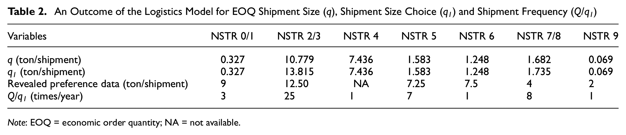
Note: EOQ = economic order quantity; NA = not available.

Table 3.

Mode Shares based on the Transport Chain Choice (ton.km)

Mode share	NSTR 0/1	NSTR 2/3	NSTR 4	NSTR 5	NSTR 6	NSTR 7/8	NSTR 9	Total	Data from MoT
Truck (alt 1)	35.86%	32.31%	47.14%	55.02%	29.77%	37.84%	49.09%	33.30%	26.22%
Train (alt 2 & alt 5)	3.28%	0.41%	2.56%	2.73%	1.73%	1.20%	14.60%	1.18%	6.55%
Vessel (alt 3 & alt 5)	55.76%	64.27%	50.14%	38.09%	63.91%	59.52%	35.18%	62.13%	67.12%
Plane (alt 4)	5.10%	3.00%	0.17%	4.16%	4.60%	1.44%	1.13%	3.39%	0.10%
Total	100%	100%	100%	100%	100%	100%	100%	100%	100%

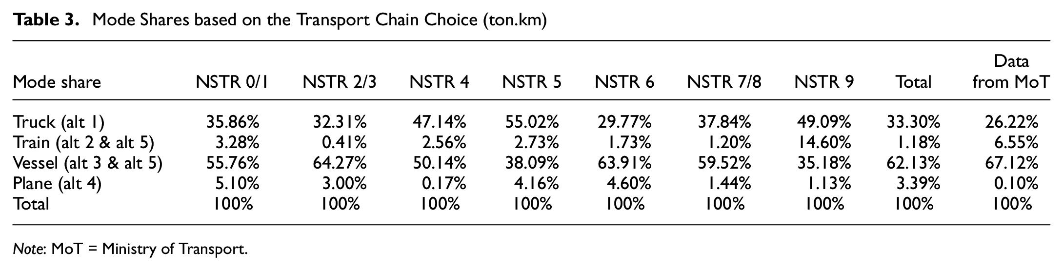
Note: MoT = Ministry of Transport.

Table 4.

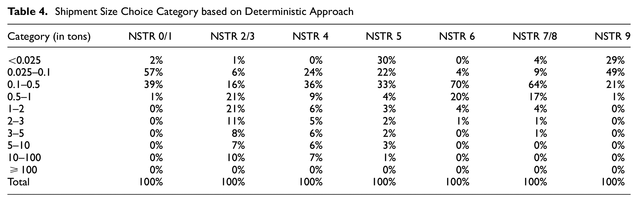
Shipment Size Choice Category based on Deterministic Approach

Category (in tons)	NSTR 0/1	NSTR 2/3	NSTR 4	NSTR 5	NSTR 6	NSTR 7/8	NSTR 9
<0.025	2%	1%	0%	30%	0%	4%	29%
0.025–0.1	57%	6%	24%	22%	4%	9%	49%
0.1–0.5	39%	16%	36%	33%	70%	64%	21%
0.5–1	1%	21%	9%	4%	20%	17%	1%
1–2	0%	21%	6%	3%	4%	4%	0%
2–3	0%	11%	5%	2%	1%	1%	0%
3–5	0%	8%	6%	2%	0%	1%	0%
5–10	0%	7%	6%	3%	0%	0%	0%
10–100	0%	10%	7%	1%	0%	0%	0%
≥100	0%	0%	0%	0%	0%	0%	0%
Total	100%	100%	100%	100%	100%	100%	100%

The values that are provided as shipment size in Table 2 are the shipment size averages of several types of f2f relationships. In the model, we assume that the relationship between zones (TaZ) could be shown by different types of f2f relationships, such as large firms to large firms (LL), large firms to medium firms (LM), large firms to small firms (LS), and so on, until small firms to small firms (SS). The distinction between types of firms is determined by the number of employees. The magnitude of the trade is assumed to be proportional to the total product of number of employees between the firms’ relation, therefore generates distinct flows for each type of firm relationship. Apart from the number of employees, these synthetic f2f relations in Indonesia’s ADA model require other input variables such as a list of provinces and zones, the number of establishments (by size category) of a certain commodity in a zone, an input–output table, and the zone-to-zone PC matrices. Consequently, by having this synthetic f2f flow, the LL relationship may have a very large shipment size because the total trade flows (Q– ton/year) are also large, whereas the SS relationship will have a modest shipment size as its Q is small. Please refer to De Jong et al. ( 6 ) for the methodology and how this methodology is applied for INTRAMOD. For the NSTR 0/1, the LL type of firms’ relation, the largest cargo size is approximately 5.08 tons per shipment, whereas the smallest shipment size is estimated to be 1.1 kg per shipment for the SS type of firms’ relation. Moreover, for bulk-type commodities such as NSTR 2/3, the largest cargo size for LL firms is up to 3,103.6 tons/shipment and the smallest shipment size is approximately 620 kg/shipment. This result is obtained by disaggregating PC into f2f flows; thus, this result is dependent on the flows between zones, and the number of establishments and their magnitude within a zone.

Continuing with Table 2, we also present the average shipment value as an outcome of the survey (median value of the RP data). The data reveal the self-reported shipment size data of firms. The median value is selected as the number of data is small, thus the median value is more representative than the mean value. In comparison with the results of the deterministic approach, the biggest shipment size for NSTR 0/1 was significantly lower than the actual RP data; this may be because of the excessive number of SS firms’ relationships within the f2f flows hypothesis. As we presume that PC flows are distributed based on the available firms’ relation option, the more the small firms’ combination, the lower the shipment size. The same condition was also applied to NSTR 9.

Table 3 displays the market share results based on the chosen transport chain in ton-kilometers. It demonstrates the mode share of four modes based on five alternative transport chains: alt1 (truck), alt 2 (truck–train–truck), alt 3 (truck–vessel–truck), alt 4 (truck–plane–truck), and alt 5 (truck–vessel–train–truck) or (truck–train–vessel–truck). The last column was added to compare the observed data in ton.km by mode for all freight commodity types in Indonesia provided by the ministry of transport (MoT). The outcome of the deterministic model is quite reasonable in comparison with the available data. All transport chain alternatives involve truck transport; consequently, when calculating the mode share for goods transported via alternative 3, for instance, these feeder flows are added to the mode share for truck transport (i.e., truck). In the meantime, the flows for alternative 5 will be implemented via truck, train, and ship. This table also reveals that sea transport is the most popular mode of transportation in Indonesia, which makes sense given that it is an archipelagic nation. The NSTR 4 demonstrates an intriguing result in which the market share of road and sea transport are nearly equal. NSTR 9 is the commodity type making the highest proportional utilization for rail transport, although across all commodity types, the primary customer of rail is NSTR 2/3. This condition in NSTR 4 may be affected by approximately 80% of the freight distribution being intra-island, so a connector mode (such as a vessel) will in many cases not be required. In the case of NSTR 9, the selection of rail as the primary mode of transport is primarily because of the extensive distribution of goods in the Java and Sumatera Island region, where rail logistics is more developed than on other islands.

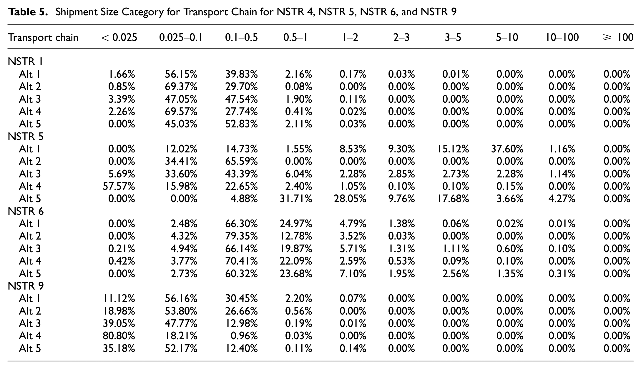
With regard to shipment size using the deterministic approach, as shown in Table 4, shipment size distributions for each commodity type could also be estimated. It can be concluded that approximately 70% of all shipment weights are less than 500 kg, with the exception of NSTR 2/3 (solid mineral) and NSTR 4 (ores and metal waste). In the case of commodity NSTR 2/3, NSTR 4, and NSTR 5 (metal products), the range of shipment sizes is quite broad, whereas NSTR 01 and NSTR 9 (consumer goods) predominantly ship small quantities. We are also interested in determining the relationship between transport chain selection and shipment size, as shown in Table 5. The table presents the distribution of shipment size based on the selected transport chain. Because of space limitations, only NSTR 1, NSTR 5, NSTR 6, and NSTR 9 will be displayed. It can be inferred from the table that air transport primarily consists of small shipments, which makes sense given that the air transport modeled here is a combination of limited-capacity freight and passenger transport. The low level of service of Indonesia’s freight rail network (i.e., the limited number of wagons and freight stations, the restricted route, and the unbalanced rail logistics development between Java and other islands) may make this mode of transport less popular for large shipments. In contrast, because of their adaptability and capacity, both land and sea transport can typically accommodate a broader range of shipment sizes.

Table 5.

Shipment Size Category for Transport Chain for NSTR 4, NSTR 5, NSTR 6, and NSTR 9

Transport chain	< 0.025	0.025–0.1	0.1–0.5	0.5–1	1–2	2–3	3–5	5–10	10–100	≥ 100
NSTR 1
Alt 1	1.66%	56.15%	39.83%	2.16%	0.17%	0.03%	0.01%	0.00%	0.00%	0.00%
Alt 2	0.85%	69.37%	29.70%	0.08%	0.00%	0.00%	0.00%	0.00%	0.00%	0.00%
Alt 3	3.39%	47.05%	47.54%	1.90%	0.11%	0.00%	0.00%	0.00%	0.00%	0.00%
Alt 4	2.26%	69.57%	27.74%	0.41%	0.02%	0.00%	0.00%	0.00%	0.00%	0.00%
Alt 5	0.00%	45.03%	52.83%	2.11%	0.03%	0.00%	0.00%	0.00%	0.00%	0.00%
NSTR 5
Alt 1	0.00%	12.02%	14.73%	1.55%	8.53%	9.30%	15.12%	37.60%	1.16%	0.00%
Alt 2	0.00%	34.41%	65.59%	0.00%	0.00%	0.00%	0.00%	0.00%	0.00%	0.00%
Alt 3	5.69%	33.60%	43.39%	6.04%	2.28%	2.85%	2.73%	2.28%	1.14%	0.00%
Alt 4	57.57%	15.98%	22.65%	2.40%	1.05%	0.10%	0.10%	0.15%	0.00%	0.00%
Alt 5	0.00%	0.00%	4.88%	31.71%	28.05%	9.76%	17.68%	3.66%	4.27%	0.00%
NSTR 6
Alt 1	0.00%	2.48%	66.30%	24.97%	4.79%	1.38%	0.06%	0.02%	0.01%	0.00%
Alt 2	0.00%	4.32%	79.35%	12.78%	3.52%	0.03%	0.00%	0.00%	0.00%	0.00%
Alt 3	0.21%	4.94%	66.14%	19.87%	5.71%	1.31%	1.11%	0.60%	0.10%	0.00%
Alt 4	0.42%	3.77%	70.41%	22.09%	2.59%	0.53%	0.09%	0.10%	0.00%	0.00%
Alt 5	0.00%	2.73%	60.32%	23.68%	7.10%	1.95%	2.56%	1.35%	0.31%	0.00%
NSTR 9
Alt 1	11.12%	56.16%	30.45%	2.20%	0.07%	0.00%	0.00%	0.00%	0.00%	0.00%
Alt 2	18.98%	53.80%	26.66%	0.56%	0.00%	0.00%	0.00%	0.00%	0.00%	0.00%
Alt 3	39.05%	47.77%	12.98%	0.19%	0.01%	0.00%	0.00%	0.00%	0.00%	0.00%
Alt 4	80.80%	18.21%	0.96%	0.03%	0.00%	0.00%	0.00%	0.00%	0.00%	0.00%
Alt 5	35.18%	52.17%	12.40%	0.11%	0.14%	0.00%	0.00%	0.00%	0.00%	0.00%

Sensitivity Analysis and Updated Assumption of the Deterministic Approach

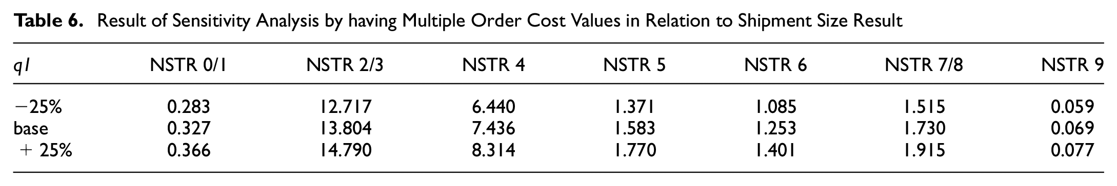
In this section, we will provide a sensitivity analysis tackling the impact of input value variations on the model’s output, which in this case is the input value of order cost variable. For this analysis, we considered three possible values for the order cost: the base order cost specified in the “Deterministic” section, 25% less than the base order cost, and 25% more than the base order cost.

Table 6 demonstrates the effect of varying order cost values on shipment value (q1). From this table, we can conclude that a decrease in order cost will result in a reduction in shipment size and an increase in shipment frequency. In contrast, a higher order cost will inevitably increase shipment volume, leading to a decrease in shipment frequency. This effect is consistent with Equation 7, which states that the order cost is proportional to shipment size. Meanwhile, changes in order cost do not have a large impact on the choice of transport chain in the deterministic approach; this may be because of the small magnitude of order cost in comparison with other cost components such as transport cost and inventory cost.

Table 6.

Result of Sensitivity Analysis by having Multiple Order Cost Values in Relation to Shipment Size Result

q1	NSTR 0/1	NSTR 2/3	NSTR 4	NSTR 5	NSTR 6	NSTR 7/8	NSTR 9
−25%	0.283	12.717	6.440	1.371	1.085	1.515	0.059
base	0.327	13.804	7.436	1.583	1.253	1.730	0.069
+25%	0.366	14.790	8.314	1.770	1.401	1.915	0.077

As previously mentioned, a problem with the original EOQ is that the average shipment size result of the model is far lower than the RP data. To cope with this condition, we applied an assumption to update the EOQ model. The first update is combining small relations shipments into a single shipment. The new assumption is that all shipments which originate from small firms will be consolidated into a single shipment (this applies to small–small [SS], small–medium [SM], and small–large [SL]). This group is aggregated for shipments with the same origin and destination zone. This update was applied to all NSTR types except for NSTR 2/3, which already had a number close to the RP data, and NSTR 4, for which we do not have the target number because of the lack of RP data. Small shipment size estimated, mostly less than 1 ton/shipment on these firms’ relation categories, rationalize this assumption.

The second variation within this version is reducing the number of receivers per sender. Theoretically, reducing the number of recipients per sender will increase the size of the shipment. This change was implemented for NSTR 0/1, NSTR 5, NSTR 6, and NSTR 9. Furthermore, if after reducing the number of receivers per sender the deterministic shipment size is still significantly below the target value, the third adjustment will be applied. The third is increasing the order costs, decreasing inventory costs, or both. The value of order cost in the model for INTRAMOD averages around £16 per order; therefore, it is preferable to order in small quantities. Order cost is the expense incurred related to placing the order which generally includes shipping (transport and transhipment cost) and handling. However, based on the EOQ equation applied in this original model, the derivative of transport cost to shipment size is zero, which means no effect of transport cost on the optimal shipment size calculation (as we assume that shipping cost is not a fixed cost as it depends on the volume of the shipment). This is, among others, a limitation in using the EOQ. Accordingly, the update on the order cost is introduced to remove or reduce this limitation. If the results of previous changes are still unsatisfactory, the final update is implemented. The final update is a restriction on the maximum shipment frequency. In the original deterministic model, the maximum shipment frequency is 365, which implies that in some cases there will be daily shipments. Consequently, tiny shipment sizes are permitted, which may lead to high transport costs. In certain NSTRs where small shipments predominate (as a result of the model), such as in NSTR 0/1 and NSTR 9, we now limit the maximum frequency of shipments. This last update will have an effect on the standard EOQ calculation: because the shipment sizes are forced to a certain value, the total logistics cost will no longer be optimal. One may, however, interpret this as adding the influence of transport cost to the EOQ calculation, which will tend to make the shipment sizes larger to reduce transport cost and benefit from economies of scale in transport. In summary, the best adjustment applied on the original EOQ model is as in Table 7; these assumptions are obtained through trial and error.

Table 7.

Changes Applied per NSTR Type for the Updated EOQ Version

EOQ version	NSTR 0/1	NSTR 2/3	NSTR 4	NSTR 5	NSTR 6	NSTR 7/8	NSTR 9
Original version	No of receiver 100	No of receiver 10	No of receiver 5	No of receiver 5	No of receiver 30	No of receiver 15	No of receiver 50
Updated version 1	Small relations are grouped into zone No of receiver 50 3 times of original order cost Inventory cost reduced by 50% Frequency of shipment max at 20 shipments	No change	No change	Small relations are grouped into zone No of receiver 1 3 times of original order cost Inventory cost reduced by 25% Frequency of shipment max at 20 shipments	Small relations are grouped into zone No of receiver 1 2 times of original order cost Inventory cost reduced by 25% Frequency of shipment max at 20 shipments	Small relations are grouped into zone Frequency of shipment max at 50 shipments	Small relations are grouped into zone No of receiver 10 3 times of original order cost Inventory cost reduced by 25% Frequency of shipment max at 20 shipments

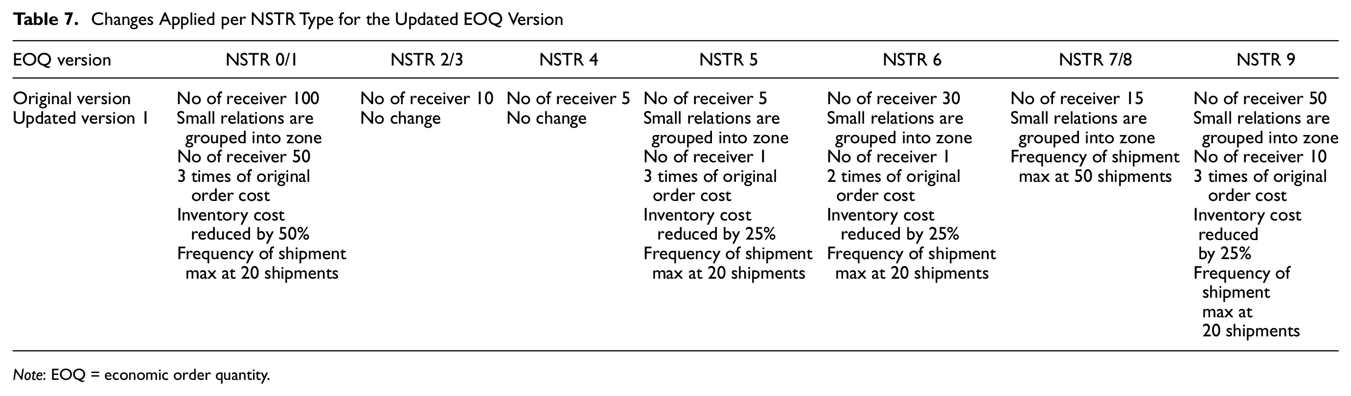
Note: EOQ = economic order quantity.

Table 8 shows the results comparison of the updated EOQ version with the previous models (modified EOQ version) on the deterministic logistics model. From Table 8, we can infer that the result of the EOQ update version is now close to the targeted shipment size values. Consequently, having different shipment sizes will affect the freight mode share and the proportion of the shipment size category as given in Table 9 and Table 10. It is inferred that the updated versions have quite different transport chain choices compared with the modified EOQ version, in which there is a lot of shifting from truck to vessel as shown in NSTR 01, NSTR 5, NSTR 6, and NSTR 9; meanwhile, NSTR 7/8 only has slight changes to the modified version (see Table 3). Considering the shipment size category, it is clearly shown that the shipment size for the updated EOQ version is leaning to bigger shipment size compared with the modified version (see Table 4). To maintain the consistent flow of this paper, all the analysis given by the deterministic logistics model will subsequently be derived from the updated EOQ version (i.e., the result provided in Table 11 for the cost elasticities analysis).

Table 8.

Shipment Size Result Comparison between Revealed Preference (RP) Data, Original EOQ Version, and the Updated EOQ Version

Variables	NSTR 0/1	NSTR 2/3	NSTR 4	NSTR 5	NSTR 6	NSTR 7/8	NSTR 9
RP data (ton/shipment)	9	12.50	NA	7.25	7.5	4	2
Original version	0.327	13.815	7.436	1.583	1.248	1.735	0.069
Updated version	4.878	NA	NA	6.471	7.095	3.512	1.115

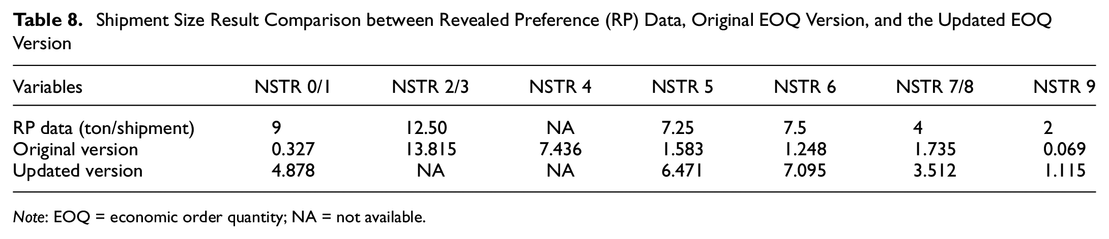
Note: EOQ = economic order quantity; NA = not available.

Table 9.

Mode Shares based on the Transport Chain Choice (ton.km) of the Updated EOQ Version

Mode share	NSTR 0/1	NSTR 2/3	NSTR 4	NSTR 5	NSTR 6	NSTR 7/8	NSTR 9	Total	Data from MoT
Truck (alt 1)	23.93%	32.31%	47.14%	30.49%	19.67%	26.87%	38.82%	30.68%	26.22%
Train (alt 2 & alt 5)	3.55%	0.41%	2.56%	4.04%	2.31%	1.41%	15.67%	1.19%	6.55%
Vessel (alt 3 & alt 5)	66.96%	64.27%	50.14%	60.97%	71.09%	69.81%	44.30%	64.65%	67.12%
Plane (alt 4)	5.56%	3.00%	0.17%	4.50%	6.93%	1.91%	1.21%	3.48%	0.10%
Total	100.00%	100.00%	100.00%	100.00%	100.00%	100.00%	100.00%	100.00%	100%

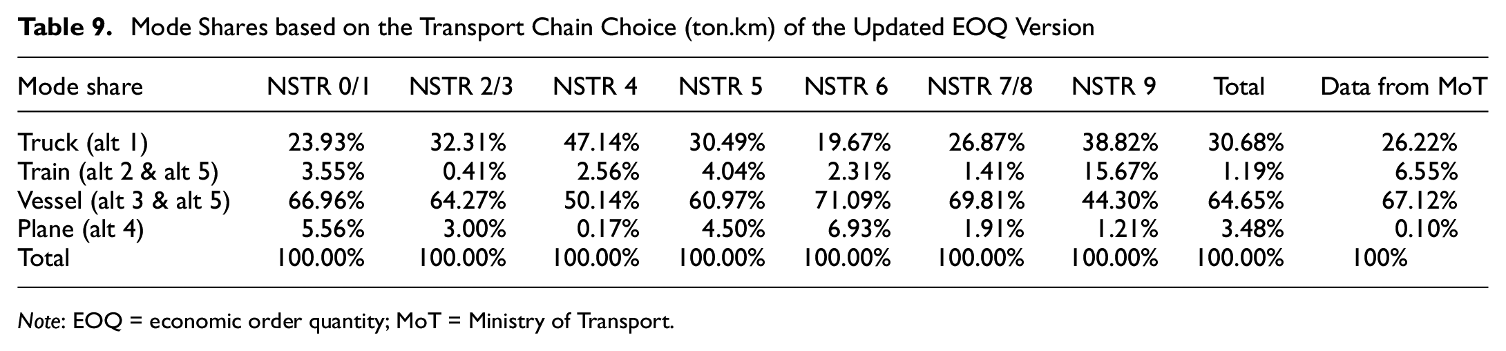
Note: EOQ = economic order quantity; MoT = Ministry of Transport.

Table 10.

Shipment Size Choice Category based on Deterministic Approach of Updated EOQ Version

Category (in tons)	NSTR 0/1	NSTR 2/3	NSTR 4	NSTR 5	NSTR 6	NSTR 7/8	NSTR 9
<0.025	0%	1%	0%	0%	0%	3%	0%
0.025–0.1	2%	6%	24%	16%	0%	2%	7%
0.1–0.5	49%	16%	36%	24%	1%	67%	50%
0.5–1	35%	21%	9%	19%	6%	19%	27%
1–2	11%	21%	6%	20%	8%	6%	13%
2–3	2%	11%	5%	3%	19%	1%	2%
3–5	0%	8%	6%	4%	20%	1%	1%
5–10	0%	7%	6%	4%	29%	1%	0%
10–100	0%	10%	7%	9%	17%	0%	0%
≥100	0%	0%	0%	1%	0%	0%	0%
Total	100%	100%	100%	100%	100%	100%	100%

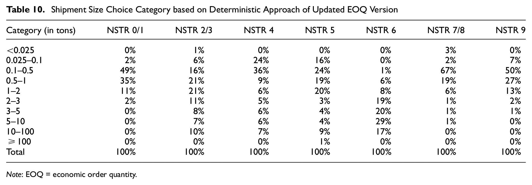
Note: EOQ = economic order quantity.

Table 11.

The Value of Time for each Main Mode of Alternative

Value of time (USD per ton/h)	RP/SP
Truck	0.104
Rail	0.301
Vessel	0.710
Plane	19.110
rail–vessel	0.496

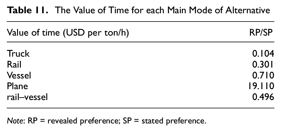
Note: RP = revealed preference; SP = stated preference.

Stochastic Approach: Discrete Choice Model Estimation for Transport Chain

This section will discuss the results of the primary estimation of the MNL model for the RP/SP data. In contrast to the deterministic model, the discrete choice in the stochastic approach only models the transport chain choice and not the shipment size choice, as data analysis for shipment size category is not yet complete. Table 12 displays the estimation results for RP data only, SP data only, and combined RP/SP data. The explanatory variables are listed in the first column, followed by the estimated coefficients using the dataset mentioned. Table 12 shows the outcome of the MNL model with variable coefficients per alternative is also displayed.

Table 12.

Estimation Results for Multinomial Logit Model for all Commodity Types

Attributes	RP data		SP data		RP/SP data
Attributes	Coefficient	t-test	Coefficient	t-test	Coefficient	t-test
asc_alt1	0.000	NA	NA	NA	0.000	NA
asc_alt2	24.387	36.351**	NA	NA	−2.808	−4.961**
asc_alt3	−2.559	−1.052	NA	NA	−1.813	−3.660**
asc_alt4	−8.665	−4.090**	NA	NA	−3.580	−3.724**
asc_alt5	−1.767	−0.218	NA	NA	−4.324	−3.157**
asc_alt1_SP	NA	NA	0.000	NA	0.000	NA
asc_alt2_SP	NA	NA	3.421	2.106**	2.916	1.494
asc_alt3_SP	NA	NA	1.379	0.921	1.307	0.898
asc_alt4_SP	NA	NA	4.352	1.758*	2.450	1.181
asc_alt5_SP	NA	NA	1.544	0.674	1.293	0.629
b_cost1	0.010	2.294**	−0.003	−6.073**	−0.003	−2.103**
b_time1	−7.754	−3.108**	−0.098	−0.501	−0.105	−0.595
b_rel1	NA	NA	0.068	5.956**	0.058	1.973**
b_cost2	0.038	1.573	−0.002	−3.705**	-0.002	−1.901**
b_time2	−22.289	−1.295	−0.244	−1.019	-0.222	−0.952
b_rel2	NA	NA	0.026	2.474**	0.022	1.555
b_cost3	−0.001	−0.221	−0.001	−1.946**	-0.001	−1.491
b_time3	−0.906	−1.191	−0.292	−3.132**	-0.263	−1.712*
b_rel3	NA	NA	0.043	3.493**	0.037	1.801*
b_cost4	0.000	−1.630	0.000	−3.012**	0.000	−1.700*
b_time4	0.339	0.345	−1.060	−1.957**	-0.551	−1.351
b_rel4	NA	NA	0.007	0.360	0.013	0.709
b_cost5	0.002	0.239	−0.001	−1.741**	-0.001	−1.392
b_time5	−2.050	−0.718	−0.248	−1.560	-0.225	−1.245
b_rel5	NA	NA	0.036	1.485	0.033	1.211
mu_RP	NA	NA	NA	NA	1.000	NA
mu_SP	NA	NA	NA	NA	1.161	2.049**
Statistics
Observations	179		624		803
LL(start)	−155.4		−733.54		−888.94
LL(final)	−61.89		−561.06		−630.78
Rho-squared (0)	0.602		0.235		0.290
Adj Rho-squared (0)	0.524		0.220		0.263

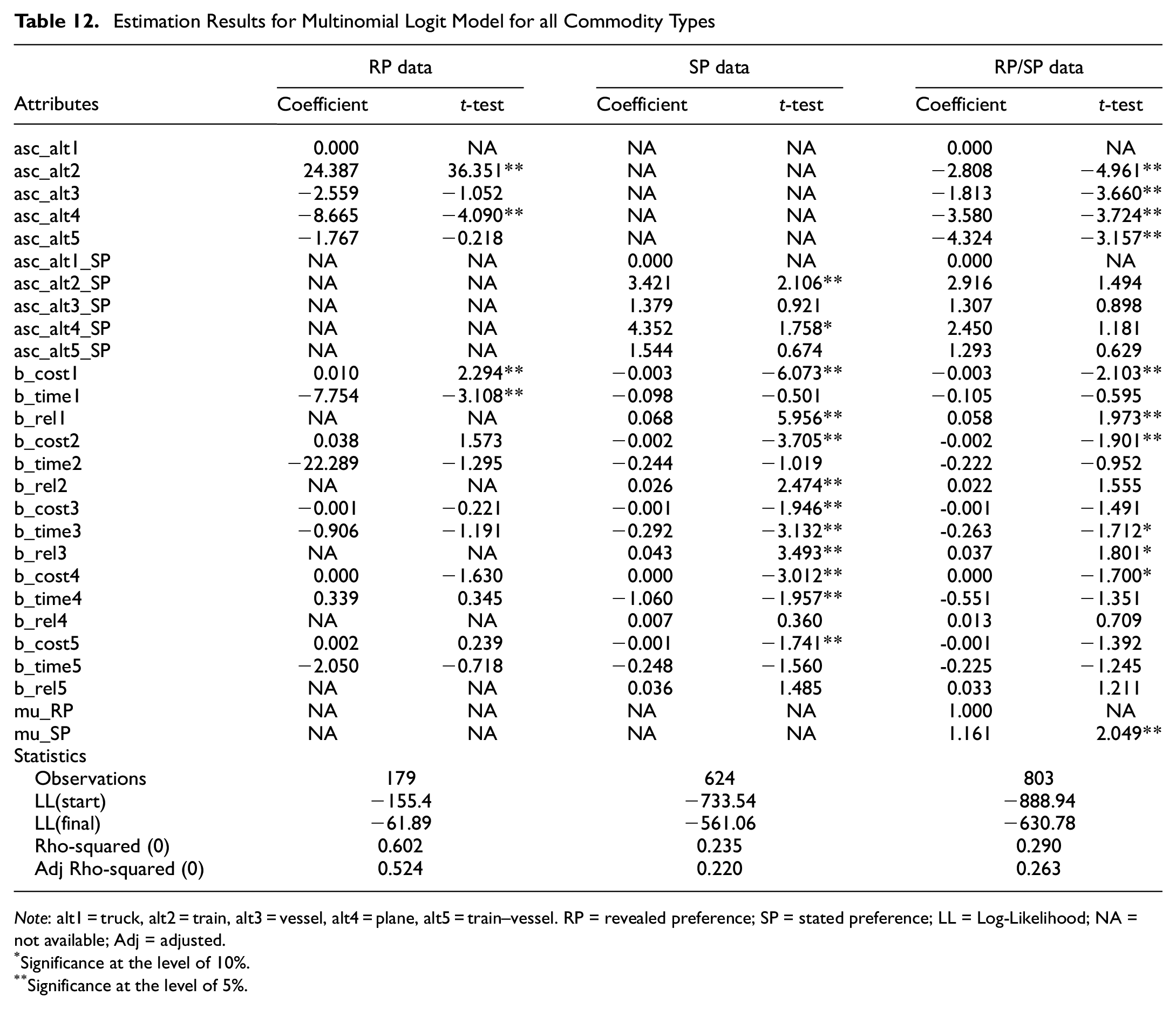
Note: alt1 = truck, alt2 = train, alt3 = vessel, alt4 = plane, alt5 = train–vessel. RP = revealed preference; SP = stated preference; LL = Log-Likelihood; NA = not available; Adj = adjusted.

Significance at the level of 10%.

Significance at the level of 5%.

The result of MNL for a single dataset of RP data does not include the reliability variables, as even though respondents provided reliability values for their preferred transport chain alternative, we lack data on the reliability of the other options. This case illustrates one of the disadvantages of relying solely on RP data, in which we lack complete information on variables of non-selected alternatives. As a result, contrary to the alternative specific constant (ASC) value, some coefficients are insignificant and have unreasonably signed explanatory variables in the results. This could be because of a small sample size of observations. On the other hand, with the exception of the ASC, the majority of explanatory variables have the expected sign when only the SP dataset is utilized. Moreover, at the 95% confidence level, the majority of the coefficients of the explanatory variables (transport cost, transport time, and reliability) are also significant.

The joint RP/SP data yield a superior ASC for the RP observation, where all coefficients are significant and have reasonable signs, whereas the ASC for the SP demonstrates the opposite. Except for the cost attribute for alternative 4, the coefficients for the transport cost, transport time, and reliability attributes have the expected sign. Further examination of the value of the RP scale parameter reveals that the scale factor is significant and greater than 1; according to Lavasani et al. in 2017, this indicates that the SP data have less noise (less variance) than the RP data ( 25 ).

This result can be used to calculate the value of time (VOT), which is calculated as βtime/βcost. The outcome of the VOT is shown in Table 11. Compared with the result by Tao and Zhu ( 23 ) and Binsuwadan et al. ( 24 ), the VOT from the SP dataset and joint RP/SP data seems plausible. The VOT for trucks is the lowest compared with other modes of transportation, such as rail, as was determined by a study Arunotayanun and Polak ( 26 ). Air transport has the highest VOT, as demonstrated by a study by Binsuwadan et al. ( 24 ). Having the lowest VOT for trucks when compared with other modes seems counterintuitive, yet this could be the case for Indonesia for various reasons. First, the rail system, which is the main competitor for trucks for land transport, is not well developed. The lack of continuous rail track and the presence of a single operator providing service, thus inducing high transport costs, are reasons why this mode is not so popular in Indonesia. Unlike the situation in many Western countries, in Indonesia rail is not a low-cost mode. A second reason is the archipelagic condition and unbalanced regional economic development between Indonesia’s west and east regions, which may contribute to the high cost of maritime transport. In sea freight shipment, it is impossible to isolate the cost of producing services in one direction from the cost of bringing the ship back. Because of the disparities in economic development between regions, eastbound trade in Indonesia is weaker than westbound trade; this imbalanced trade leads to the emergence of a phenomenon in which the fronthaul trip may bear the entire cost of round trips, whereas the backhaul trip can only cover a small portion of transport costs.

The comparison between the results from the MNL model and the CFS data is given in Table 13. However, the data given by the MoT are not at the shipper level, so we could not perform an apple-to-apple comparison. Table 13 provides an estimation of the transport chain’s choice of shipper based on the sample size we gathered in RP survey. It is shown in Table 13 that the result of the stochastic approach is quite close to the data from the transport ministry, in which sea transport has the biggest share, whereas the lowest share is for air transport.

Table 13.

Mode Share Comparison between RP Data using Multinomial Logit Model (in Ton.km)

Mode share	RP estimation	SP estimation	MoT
Truck (alt 1)	32.19%	13.18%	26.22%
Train (alt 2 & alt 5)	9.77%	11.73%	6.55%
Vessel (alt 3 & alt 5)	51.88%	74.94%	67.12%
Plane (alt 4)	6.16%	0.14%	0.10%
Total	100%	100%	100%

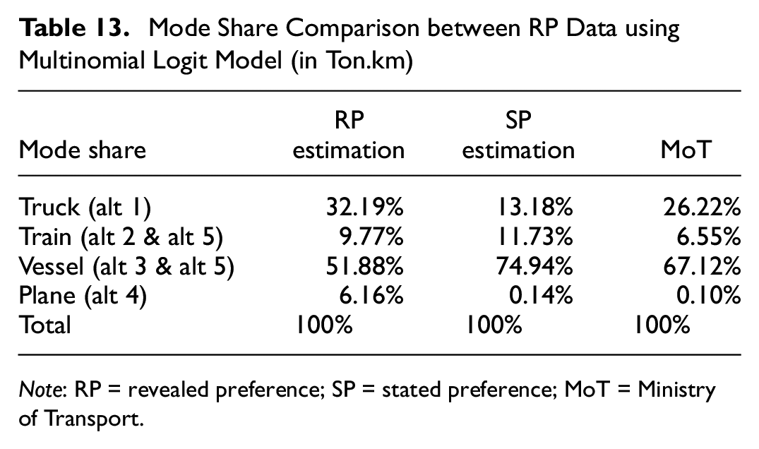
Note: RP = revealed preference; SP = stated preference; MoT = Ministry of Transport.

Cost Elasticities

A fascinating aspect of developing a model is understanding the response of the outcome, here the selected transport chain alternative, to changes in the input data (i.e., simulation or model application). In this section, we compare the deterministic model with the stochastic model (joint RP/SP model) in relation to demand elasticities for all transport chain alternatives, relative to transport cost changes. The cost changes for calculating the elasticities are assumed to be segregated, which means that the increase in transport cost for alternative 1 (i.e., truck) will have no effect on the cost of the other alternatives, despite each transport chain alternative including truck mode. The effect of transport cost changes in the selected transport chain will then be examined at the ton-kilometers per alternative.

The results of direct and cross-elasticities for deterministic and stochastic approaches are displayed in Table 14. The direct elasticities are highlighted in bold. In the deterministic approach, elasticities are differentiated based on the type of commodity, whereas in the stochastic approach, there are insufficient data to distinguish commodities, resulting in a single value. However, although the estimation results from the RP–SP model are used here, these elasticity values are calculated separately as RP and SP results. The direct elasticities for the deterministic model have a reasonable sign, as shown in Table 14. There are too many perfectly inelastic demands in NSTR 5, resulting in an intriguing result. The inelastic condition indicates that changes in commodity costs will have no effect on the selected alternative; this is to be expected for NSTR 5 (metal products), which involves considerable heterogeneity (i.e., shipping steel in the form of a beam differs from shipping steel in the form of a coil, and shipping steel for construction may also differ, such that the nature of the shipment may vary based on its form). NSTR 9 also has some similar characteristics. However, the majority of the products in this category are consumables such as textiles, electronics, and wood products that do not require special handling during shipment; therefore, the inelastic demand may be evidence of sticky choice problems in the deterministic approach, where the model is too stable, and the chosen alternative has significantly lower logistics costs than the second-best alternative. Contrary to the deterministic method, this phenomenon does not exist in the stochastic model.

Table 14.

Direct and Cross-demand Elasticities in Deterministic and Stochastic Approaches with Respect to the Changes of Alternative’s Cost

NSTR	Alternative	alt 1		alt 2		alt 3		alt 4
NSTR	Alternative	10%	−15%	10%	−15%	10%	−15%	10%	−15%
Deterministic
NSTR 01	Alt 1	−0.32	−0.72	0.31	0.24	0.13	0.13	0.00	0.00
	Alt 2	0.32	0.27	−0.30	−0.59	0.20	0.05	0.00	0.00
	Alt 3	0.01	0.42	0.00	0.35	−1.00	−0.66	0.00	0.00
	Alt 4	0.00	0.00	−0.01	−0.01	0.01	0.00	0.00	0.00
	Alt 5	0.00	0.03	0.00	0.00	0.66	0.47	0.00	0.00
NSTR 5	Alt 1	−0.01	−0.01	0.00	0.00	0.00	−0.05	0.00	0.00
	Alt 2	0.00	0.01	0.00	0.00	0.00	0.00	0.00	0.00
	Alt 3	0.01	0.00	0.00	0.00	0.00	−3.06	0.00	0.00
	Alt 4	0.00	0.00	0.00	0.00	0.00	−0.02	0.00	0.00
	Alt 5	0.00	0.00	0.00	0.00	0.00	3.14	0.00	0.00
NSTR 9	Alt 1	−1.12	−2.10	1.46	0.78	0.09	0.20	0.00	0.00
	Alt 2	1.10	1.43	−1.44	−1.93	0.40	0.26	0.00	0.00
	Alt 3	0.00	0.44	−0.01	1.16	−0.92	−0.83	0.00	0.00
	Alt 4	0.00	0.01	0.00	−0.01	0.00	0.00	0.00	0.00
	Alt 5	0.03	0.22	−0.01	0.00	0.44	0.37	0.00	0.00
Stochastic
RP elasticitiesAll commodities	Alt 1	−0.14	−0.19	0.02	0.02	0.00	0.00	0.01	0.01
	Alt 2	0.95	1.41	−0.81	−0.74	0.82	0.78	0.01	0.01
	Alt 3	0.36	0.53	0.02	0.02	−0.27	−0.25	0.15	0.15
	Alt 4	0.37	0.53	0.02	0.02	0.50	0.42	−0.85	−0.76
	Alt 5	0.13	0.22	0.01	0.01	0.72	0.64	0.20	0.21
SP elasticitiesAll commodities	Alt 1	−0.51	−0.45	0.21	0.19	0.05	0.04	0.02	0.02
	Alt 2	0.33	0.32	−0.48	−0.42	0.05	0.06	0.03	0.03
	Alt 3	0.33	0.33	0.22	0.24	−0.45	−0.38	0.14	0.13
	Alt 4	0.28	0.27	0.22	0.22	0.22	0.20	−0.60	−0.54
	Alt 5	0.23	0.25	0.13	0.18	0.36	0.31	0.20	0.21

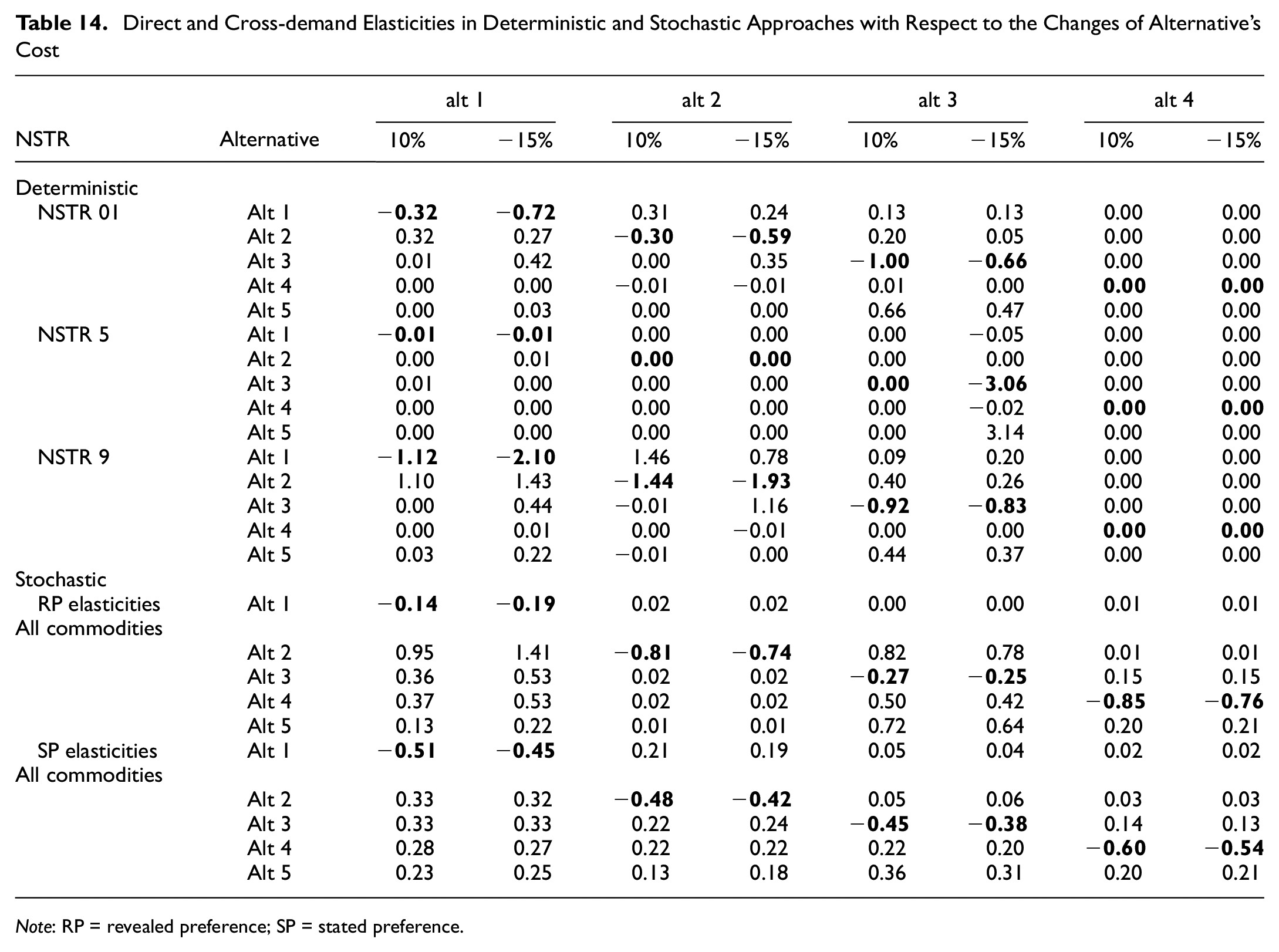
Note: RP = revealed preference; SP = stated preference.

Considering the elasticities results for each mode of transport in the deterministic approach, it is possible to conclude that freight modes have inelastic demand. However, some modes have absolutely low elasticities (such as air transport), which demonstrates a sticky choice behavior, whereas others can suddenly change their share (such as sea transport in the scenario with 15% off the alt 3 cost), which demonstrates a flip-flopping behavior. In the stochastic model, the elasticities for all modes are relatively elastic and stable.

Conclusion and Further Work

This paper’s findings provide the foundation for the development of a logistics model for Indonesia’s national freight transport model system (INTRAMOD). Starting with the deterministic method to estimate the transport chain selection and shipment size, the findings were comparable to the MoT’s published freight mode market share. The deterministic logistics model assumes that shippers select the most cost-effective total logistics cost. A modified EOQ (i.e., making use of twenty possible shipment frequencies) applied to the consolidation assumption yielded plausible results in simulating the shipper’s decision about the transport chain and shipment size. In addition, we also perform the comparison in view of mode share between the results of the modified EOQ with the RP data. The result is that the modified EOQ predicts shipment sizes far smaller than the data. Consequently, we updated the EOQ into a new version by applying some adjustments and assumptions to the cost variables so that the results are now closer to the data. The outcome of the deterministic method also reveals the distribution of shipment size for each commodity category and how shipment size influences the selection of the transport chain. In conclusion, a natural resource commodity has a greater variation in shipment size, whereas consumable items are typically transported in small quantities. In addition, it has been determined that small shipments utilize air transport exclusively because of the limited capacity of air transport. Meanwhile, the popularity of rail transport for large shipment sizes may be adversely affected by the low level of service of the freight rail network in Indonesia. On the other hand, road and sea transport have a wider range of cargo size variations owing to their adaptability and capability of handling large capacity.

This work confirms that one of the issues with the deterministic approach to the logistics model, as presented in transport chain simulation (results for elasticity), is the occurrence of “sticky” and “flip-flop” behaviors to some degree. Such overly stable behavior occurs when the logistics cost function for the selected alternative is significantly distinct from that of the second-best alternative, so that even substantial changes in cost have no influence on demand. On the other hand, relatively flat cost functions for alternatives are the main reason for flip-flop behavior. The disaggregate stochastic logistics model is developed in an effort to address this issue. The outcome of the elasticities demonstrates that the stochastic approach is a possible solution to this problem. However, we need to bear in mind that the stochastic approach does require detailed data on shipment characteristics, which is rarely available for developing countries such as Indonesia.

In addition, this paper included research into the construction of a stochastic logistics model for INTRAMOD. Using the RP/SP data, parameter estimation was carried out with a basic MNL model with different coefficients for each attribute and alternative. In contrast to the deterministic model, the current stochastic approach currently only considers the choice of shipper in the transport chain and not the shipment size. The results of the model indicate a significant SP to RP scale parameter with a value greater than 1, indicating greater variations in the RP data. The parameters of the MNL model for the RP dataset alone suggest significant and appropriate ASC values, but odd and insignificant transport time and cost coefficients. In contrast, the MNL result with only SP data reveals an unexpected ASC value, with alternative 2 (rail) and alternative 4 (plane) being the most attractive modes of transport for freight shipment if the cost, time, and reliability differences are controlled for (this may not be portraying the real situation). Nonetheless, it exhibits credible and substantial coefficient parameter values. Consequently, utilizing both RP and SP datasets is anticipated to enhance the stochastic model. The MNL result of the combined dataset demonstrates a small improvement over the previous analysis. With regard to the VOT calculation, the joint RP/SP model is consistent with the findings of a prior study on the freight mode VOT for Indonesia.

Further research will be conducted to investigate more complex stochastic methods, such as modeling the discrete choice of joint transport chain and shipment size. Other model specifications, such as the nested logit model, may also be estimated alongside the MNL model. Finally, a comprehensive logistics model for INTRAMOD using both deterministic and stochastic approaches will be utilized later on to estimate aggregated OD flows.

Footnotes

Acknowledgements

The authors wish to thank the Directorate of Higher Education, Ministry of Education and Culture, the Republic of Indonesia for financial support for this research.

Author Contributions

The authors confirm contribution to the paper as follows: study conception and design: LNNH, GJ, AW; data collection: LNNH, GJ, AW; analysis and interpretation of results: LNNH, GJ, AW; draft manuscript preparation: LNNH, GJ, AW. All authors reviewed the results and approved the final version of the manuscript.

Declaration of Conflicting Interests

The author(s) declared no potential conflicts of interest with respect to the research, authorship, and/or publication of this article.

Funding

The author(s) disclosed receipt of the following financial support for the research, authorship, and/or publication of this article: The authors also wish to thank the University of Leeds and Universitas Sebelas Maret Surakarta for the support on this publication with research grant number 254/UN27.22/PT.01.03/2022.

ORCID iDs

Lydia Novitriana Nur Hidayati

Anthony Whiteing

References

De Jong

Vierth

Tavasszy

Ben-Akiva

Recent Developments in National and International Freight Transport Models within Europe. Transportation, Vol. 40, No. 2, 2013, pp. 347–371. https://doi.org/10.1007/s11116-012-9422-9.

Davydenko

Logistics Chain in Freight Transport Modelling. Faculty of Technology, Policy, and Management, Delft University of Technology, Netherland, 2015.

Halim

R. A.

Strategic Modelling of Global Container Transport Network. Delft Univeristy of Technology, Netherland, 2016.

Huber

Transport Chain Choice Modelling in Freight Transport Demand Models. Open Science Journal, Vol. 2, 2017. https://doi.org/10.23140/RG.2.3.3441.0967.

Abate

Vierth

Karlsson

Jong

G. D.

Baak

Estimation and Implementation of Joint Econometric Models of Freight Transport Chain and Shipment Size Choice. CTS - Centre for Transport Studies (KTH and VTI), Stockholm, 2014.

De Jong, Gerard , et al. Technical Report on the Further Development of a Logistics Module in the Norwegian and Swedish National Freight Model Systems. Significance, Netherland, 2007.

Ben-Akiva

De Jong

The Aggregate–Disaggregate–Aggregate (ADA) Freight Model System. In Recent Developments in Transport Modelling, ( Moshe

B. A.

Hilde

Eddy van de

, eds.), Emerald Group Publishing Limited, Bingley, 2008, pp. 117-134.

Abate

Vierth

Karlsson

de Jong

Baak

A Disaggregate Stochastic Freight Transport Model for Sweden. Transportation, Vol. 46, 2018, pp. 671–696. https://doi.org/10.1007/s11116-018-9856-9.

Huber

Klauenberg

Thaller

Consideration of Transport Logistics Hubs in Freight Transport Demand Models. European Transport Research Review, Vol. 7, 2015, pp. 1-14. https://doi.org/10.1007/s12544-015-0181-5.

10.

Jensen

A. F.

Thorhauge

de Jong

Rich

Dekker

Johnson

Cabral

M. O.

Bates

Nielsen

O. A.

A Disaggregate Freight Transport Chain Choice Model for Europe. Transportation Research Part E: Logistics and Transportation Review, Vol. 121, 2019, pp. 43-62. https://doi.org/10.1016/j.tre.2018.10.004.

11.

De Tremerie

L. M. F.

An Application of Quantitative and Qualitative Methods in Freight Mode Choice Modelling. Institute for Transport Studies, University of Leeds, 2018.

12.

Tuğdemir Kök

Deveci

Freight Transport Mode Choice with Stated Preference Method: A Systematic Literature Review. Mersin University Journal of Maritime Faculty, Vol. 1, 2019, pp. 17-29.

13.

Abate

Vierth

De Jong

, Joint Econometric Models of Freight Transport Chain and Shipment Size Choice. CTS - Centre for Transport Studies (KTH and VTI), Stockholm, 2014.

14.

Filla

F. R.

Pemilihan Moda Transportasi Darat Dalam Mendukung Efektivitas Pengiriman Barang. Jurnal Bisnis, Logistik Dan Supply Chain (BLOGCHAIN), Vol. 2, No. 2, 2022, pp. 52-57. https://doi.org/10.55122/blogchain.v2i2.526.

15.

Nugroho

M. T.

Stated Preference Study of Port and Inland Mode Choice for Containerized Export from Java. Institute for Transport Studies, The University of Leeds, 2015.

16.

Tavasszy

Ruijgrok

Davydenko

, Incorporating Logistics in Freight Transport Demand Models: State-of-the-Art and Research Opportunities. Transport Reviews, Vol. 32, No. 2, 2012, pp. 203-219. https://doi.org/10.1080/01441647.2011.644640.

17.

De Jong

de Bok

Thoen

Seven Fat Years or Seven Lean Years for Freight Transport Modelling? Developments Since 2013. Journal of Transport Economics and Policy, Vol. 55, 2021, pp. 124-140.

18.

Combes

Empirical Evaluation of Economic Order Quantity Model for Choice of Shipment Size in Freight Transport. Transportation Research Record: Journal of the Transportation Research Board, 2012. 2269: 92-98.

19.

Train

Discrete Choice Methods with Simulation. Cambridge University Press, 2009.

20.

Caspersen

Johansen

B. G.

Hovi

I. B.

de Jong

Norwegian Logistics Model: Moving from a Deterministic Framework to a Random Utility Model. TØI Report (1538/2016). Institute of Transport Economics, Norway, 2016.

21.

De Jong

Bakker

Pieters

New Values of Time and Reliability in Freight Transport in The Netherlands. Association for European Transport, Netherlands, 2004.

22.

De Jong

Kouwenhoven

Bates

Koster

Verhoef

Tavasszy

Warffemius

New SP-Values of Time and Reliability for Freight Transport in the Netherlands. Transportation Research Part E: Logistics and Transportation Review, Vol. 64, 2014, pp. 71-87. https://doi.org/10.1016/j.tre.2014.01.008.

23.

Tao

Zhu

Meta-Analysis of Value of Time in Freight Transportation: A Comprehensive Review Based on Discrete Choice Models. Transportation Research Part A: Policy and Practice, Vol. 138, 2020, pp. 213-233. https://doi.org/10.1016/j.tra.2020.06.002.

24.

Binsuwadan

De Jong

Batley

Wheat

The Value of Travel Time Savings in Freight Transport: A Meta-Analysis. Transportation, Vol. 49, 2022, pp. 1183-1209. https://doi.org/10.1007/s11116-021-10207-2.

25.

Lavasani

Hossan

M. S.

Asgari

Jin

Examining Methodological Issues on Combined RP and SP Data. Transportation Research Procedia, Vol. 25, 2017, pp. 2330-2343. https://doi.org/10.1016/j.trpro.2017.05.218.

26.

Arunotayanun

Polak

Taste Heterogeneity and Market Segmentation in Freight Shippers’ Mode Choice Behaviour. Transportation Research Part E: Logistics and Transportation Review, Vol. 47, 2011, pp. 138-148. https://doi.org/10.1016/j.tre.2010.09.003.

Logistics Model for Indonesia’s National Freight Model System: From a Deterministic to a Stochastic Framework

Abstract

Keywords

Logistics Model

Deterministic

Stochastic

Moving from Deterministic to Stochastic

Data Analysis

Results from the Deterministic Approach

Deterministic Transport Chain and Shipment Size Choice

Sensitivity Analysis and Updated Assumption of the Deterministic Approach

Stochastic Approach: Discrete Choice Model Estimation for Transport Chain

Cost Elasticities

Conclusion and Further Work

Footnotes

Acknowledgements

Author Contributions

Declaration of Conflicting Interests

Funding

ORCID iDs

References