Sage Journals: Discover world-class research

Abstract

This paper focuses on the potential of HOT lanes (high-occupancy toll lanes) in Germany. For this, various scenarios were defined and simulated on a synthetic road network that adheres to German guidelines. The results demonstrated that HOT lanes offered travel time advantages for carpoolers and HOT vehicles but led to longer travel times for single-occupancy vehicles and trucks. Scenarios with higher costs per kilometer generally reinforced the promotion of high-occupancy vehicles and encouraged a shift toward public transport. In contrast, low cost rates had a negative impact on the desired modal split, as the low cost of using the HOT lane became an incentive for comfortable HOT travel rather than carpooling or using public transport. With regard to CO₂ and NOx emissions, we demonstrated the unexpected consequences of HOT lanes, when the general traffic flow worsened. In all scenarios, the emissions for both groups were consistently higher than in the baseline scenario without a managed lane, because of the reduced traffic flow. Overall, scenarios with higher costs per kilometer were more favorable in relation to emissions, as the displacement effect toward carpooling vehicles and public transport reduced the overall number of vehicles in the system. This issue may need to be addressed with the implementation of intelligent traffic management systems, especially those that can influence speed. Taking a comprehensive view of the results, HOT lanes in Germany offer the potential for improving traffic conditions and optimizing modal split. However, the limitations of their application must be taken into account.

Keywords

operations managed lanes high-occupancy tolls microscopic traffic simulation

The field of managed lanes is vast, and so far, no country in the world has implemented all facets of managed lanes on a comprehensive scale. Depending on the traditions in individual countries, the focus is placed on different measures. For example, high-occupancy vehicle (HOV) lanes and high-occupancy toll (HOT) lanes have been standard traffic management procedures in the United States for several years, but they are currently rarely used in Europe and not at all in Germany ( 1 ). Some potential of HOV lanes has been recognized, for example Weyland et al. presented a concept, envisioning a HOV lane that would be opened during peak hours, similar to the concept of limited hard-shoulder running ( 2 ). Our approach, however, comes from a different perspective, assuming that no additional road space is created or allocated for the managed lane. Instead, one lane is taken from regular traffic and provided to privileged road users. Since HOV lanes often have available capacity even during peak hours ( 3 ), resulting in underutilization of road space, our research focuses on a HOT lane, even though tolls or road usage fees are not yet levied on public roads in Germany.

Given that managed lanes using pricing strategies and tolls have not been implemented in Germany, there are no existing references on how people, especially commuters, would react to a HOT lane. To address this, we conducted a preliminary survey to explore the needs and requirements of commuters with regard to managed lanes ( 4 ). In addition, we had data from pilot projects in other European countries that have recently designated HOV-/HOT lanes, which served as a framework for our study ( 5 – 8 ). Based on these results, the present study utilized various simulations using the Aimsun software to test different scenarios and analyze their impacts on traffic flow, mode choice, and several environmental parameters.

Motivation

In Germany, Europe, and worldwide, traffic volumes are steadily increasing ( 1 , 9 ). Concurrently, investments in new road construction and expansion have been steadily declining since the 1990s ( 3 , 10 ). Several factors have contributed to this trend, including increased maintenance costs for existing road networks and budget constraints in several regions. Moreover, rising environmental regulations, changing perceptions among a vocal segment of the population, and increasing competition for available land pose challenges for road planning and construction.

Given these circumstances, the task in the coming years lies in efficiently utilizing existing transportation networks. One approach that has proven successful internationally but has seen limited implementation in Europe and especially in Germany is the adoption of HOV- and HOT lanes. We recognize substantial potential for implementing such lanes in the German road network and have conducted a survey among German commuters and presented the findings at TRB 2023 ( 4 ) and ISFO 2023 ( 11 ). Building on these insights, we derived a formula to determine modal choice, providing the proportions of public transport (PT), HOV, HOT, and single-occupancy vehicle (SOV) usage under various conditions. Following these results, this paper describes the specific effects that a HOV-/HOT lane could have on traffic flow in the German road network. This includes investigating the optimal toll costs, examining the impact on traffic flow under different conditions, and assessing the environmental effects on carbon dioxide (CO₂) and nitrogen oxides (NOx) emissions.

Data and Traffic Model

Our road network is based on the German Manual for the Design of Traffic Facilities (HBS 2015, hereafter HBS; 12 ), as shown in Figure 1. This is a synthetic section, representing average values of German freeways. It consists of an approximately 18-km long stretch, encompassing two freeway interchanges (connecting different freeways), Interchanges 1 and 6, and four junctions (simple ramp), 2 to 5, intersecting the stretch at irregular intervals. Points A and B represent the entrance and exit points of the roadway network.

Figure 1.

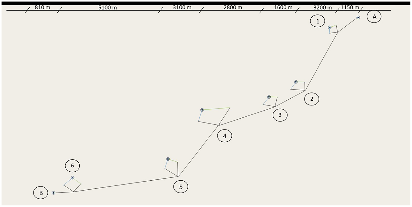
Simulation network: own network on Aimsun based on a HBS-network ( 12 ).

The road configuration consists of three lanes per direction, or a six-lane cross-section in total. The simulation focuses only on the morning peak direction, thus considering only one direction of travel with three lanes in detail. Within this study, the managed lane analyzed was exclusively the left-hand lane, which corresponds to the location of the majority of managed lanes worldwide ( 13 ). The managed lane begins at Interchange A and terminates at Interchange B and continues from there as a regular lane. The managed lane thus describes a section of road between two freeway interchanges, which corresponds to a realistic project scope in practice. The general conditions of such a subsection can be considered uniform enough and suitable for the implementation of a managed lane.

In relation to traffic load, the numbers are designed to represent Quality Level D, according to HBS, throughout the entire network ( 12 , 14 ). This implies dense traffic conditions where unrestricted driving/overtaking is not always possible. However, the overall traffic state remains stable. In the present model, commuters can choose from four different transportation modes (SOV, HOV, HOT, PT), with PT users not utilizing the freeway and multiple travelers (2+) sharing a HOV. The numerical values are adjusted such that in a baseline scenario in which no managed lane is implemented, Quality Level D is maintained. Different scenarios may result in varying quality levels, depending on the outcomes.

Traffic load is described in Table 1. The table presents the number of individuals with their origin–destination (O-D) relationships occurring in the peak hour within the network. In this context, A represents the number of commuters entering the model at the beginning of the network, whereas B indicates the count of individuals leaving the network. For this study, heavy-duty traffic was assumed to be constant at 10% of the vehicles entering at A. The distribution within the O-D matrix remained constant relative to all scenarios, even when the number of vehicles varied. Some simplifications were made in the entire system. Firstly, it was assumed that the distribution of different transportation modes at each junction remained constant and that, for example, HOVs did not preferentially select a specific junction. The vehicle types HOV and HOT were ascribed the same properties, even though HOT vehicles tended to achieve higher speeds in practice. The proportion of heavy vehicles also remained constant throughout the stretch.

Table 1.

Total Origin–Destination Matrix of Commuters in the Network seen in Figure 1 during Peak Hour Without Trucks

	1 off	2 off	3 off	4 off	5 off	6 off	B off
A on	365	292	657	146	146	292	5.329
1 on	NA	253	261	90	49	65	90
2 on	NA	NA	391	57	25	114	44
3 on	NA	NA	NA	279	236	182	365
4 on	NA	NA	NA	NA	147	535	367
5 on	NA	NA	NA	NA	NA	277	616
6 on	NA	NA	NA	NA	NA	NA	872

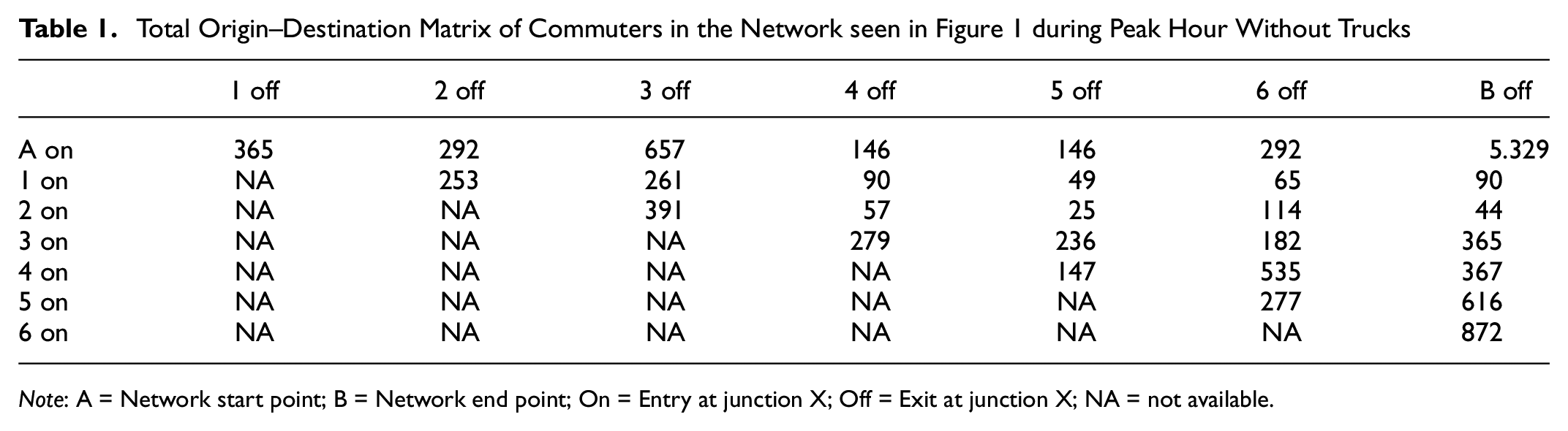
Note: A = Network start point; B = Network end point; On = Entry at junction X; Off = Exit at junction X; NA = not available.

The distribution within the O-D matrix in Table 1 was generated using random numbers. Traffic was reduced in some places and increased in others, so the impact of increased numbers of vehicles entering or exiting could be evaluated. The largest volume of traffic occurred in the section between Junctions 5 and 6. The relative O-D matrix remained constant in all simulation runs. This meant that the traffic volume for the different simulation runs could vary, but always followed the distribution shown above. The provided data yielded varying levels of congestion for different segments of the roadway. The maximum congestion was in the section between Junctions 5 and 6, which was evident in the analyses below. Between Interchanges 2 and 3, the traffic slightly decreased, resulting in fewer vehicles within that section. These deliberate variations in congestion levels were chosen to ensure a comprehensive analysis.

The allocation of modal choice, $p$ ,was determined using the following equations, presented during ISFO 2023 ( 11 ):

p_{HOT} = 0.0751 ‒ 0.000738 \times x_{1} ‒ 0.00432 \times x_{2} + 0.00461 \times x_{3}

(1)

p_{HOV} = 0.137 + 0.0161 \times x_{1} + 0.00491 \times x_{2} + 0.0101 \times x_{3}

(2)

p_{SOV} = 0.493 + 0.0194 \times x_{1} - 0.00377 \times x_{2} - 0.0181 \times x_{3}

(3)

p_{PT} = 0.279 - 0.0336 \times x_{1} + 0.00340 \times x_{2} + 0.00430 \times x_{3}

(4)

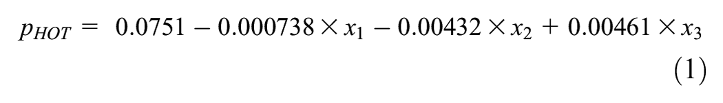
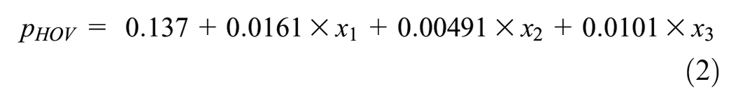
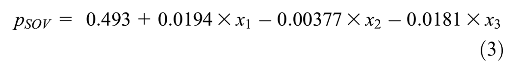
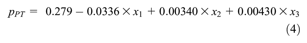
where

x₁ describes the travel distance in a clustered way,

x₂ stands for the toll costs called, and

x₃ indicates the travel time gain that can be achieved using a managed lane.

We utilized a synthetic traffic model with the following assumptions:

- The HOT lane may be used by HOVs and SOVs willing to pay, as well as PT vehicles if provided.

- The following vehicle types with the specified properties and designations were used in the simulation:

○ PT

○ HOV: allowed to use the HOT lane free of charge

○ HOT vehicle: a SOV paying the toll for the HOT lane

○ SOV: not paying the toll for the HOT lane

- The initial number of travelers, divided into PT, SOVs, HOVs, and HOT vehicles, was 7,300 persons.

- The proportion of heavy vehicles remains constant at 10% of the initial traffic load.

- All commuters in the system travel total distances of between 10 and 30 km, solely on the freeway.

- For commuters forming carpooling arrangements or using PT, there is an induced traffic of 2.5% added to the SOV category. Distribution concerning the O-D relationship remains unchanged.

- PT users opt for rail-based transportation or alternative routes, and therefore do not appear on the observed freeway segment.

Scenarios and Modeling

The presented simulations were conducted using Aimsun Next 22.0.2 software. For each scenario, a minimum of 10 simulation runs were performed, ensuring compliance with the guidelines outlined ( 15 ). The scenarios involved various cost rates per kilometer to be paid by HOT vehicles, ranging from 0.1 to 1.0 €/km. In this study, the calculation of travel cost considered the distance between the entry and exit points. Thus, it did not matter if a vehicle changed lanes more frequently, resulting in a longer distance traveled, or followed the shortest path. The evaluation aimed to provide robust results through interpolation, even for intermediate values. A baseline scenario was additionally simulated to serve as a reference to assess the impacts of the managed lane.

The network was synthetic, based on a proposal from the HBS ( 12 ), created to depict a representative freeway section and to present the results in a highly transferable manner. The synthetic model was calibrated through validation of the baseline scenario. This involved iteratively adjusting the model parameters across various simulation runs at a baseline traffic volume until a realistically representative traffic flow was observed. Extensive real-world traffic data ( 14 ) were utilized to establish a solid foundation for the model. General data from the Federal Statistical Office in Germany, as well as detailed information such as detector data, were employed. The data encompassed traffic flow, vehicle types, and speeds, which were subsequently integrated into the road network modeled.

Following this, microscopic traffic-flow simulations were conducted and analyzed. Based on the available information and simulation results, the parameters of the simulation were adjusted to achieve the most accurate representation of traffic. These parameters included vehicle dynamics, driver behavior, and following distances. Minor optimizations were additionally made to the road network.

This process was iteratively repeated several times, also for different scenarios, until a satisfactory agreement between real data and simulations was achieved for various traffic indicators such as traffic congestion, average speed, and travel times. This process led to a consistent model design, which, similar to HBS ( 12 ), allowed for easy transferability to other traffic situations.

The simulations focused on the peak hour. A 1-h ramp-up phase was initially simulated, followed by the peak hour and then a winding-down phase. For the evaluation, only vehicles that entered the system between the first and second hour were considered.

Results, Benefits, and Impacts

In Germany, HOT lanes are primarily associated with expectations in three thematic areas that represent the most significant challenges in the German transport sector:

Modal shift in favor of sustainable mobility,

Optimizing travel times, and

Reducing emissions.

These will therefore be examined in more detail below. In the context of choice of transportation mode and route, some road users may opt not to use the managed lane on short distances, even if they are entitled to, as they may undervalue the benefits of travel time gain compared with the negative effects, such as lane changes. As a result, we emphasize evaluating routes with larger travel time gains in the following analyses. Values with travel time gains under 120 s were excluded from the evaluation in the simulations and were only qualitatively recorded. An exemplary table with O-D relationships for one scenario is described in the following section and shown in Table 2.

Table 2.

Travel Time Gain (min) for 0.5 €/km

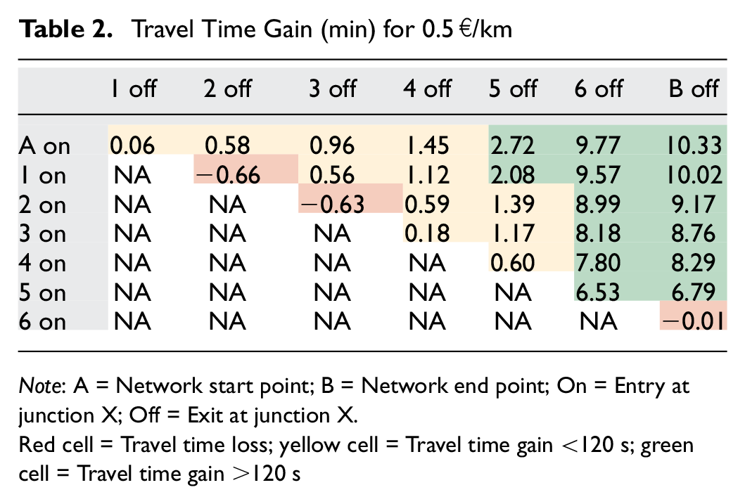
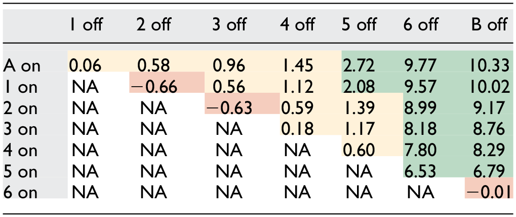
Note: A = Network start point; B = Network end point; On = Entry at junction X; Off = Exit at junction X.

Red cell = Travel time loss; yellow cell = Travel time gain <120 s; green cell = Travel time gain >120 s

Figure 2 depicts the relationship between expected travel time gain and actual travel time gain, evaluated for vehicles traveling through the entire synthetic network with the option to switch to the HOT lane for a cost of 0.5 €/km. To achieve this, starting from an initial value, microscopic simulation runs were conducted for the scenario. An expected travel time for different modes of transportation was assumed and subsequently calculated in the simulation. The results were then used as the expected travel time for the next simulation. The x-axis of the graph represents the expected travel times, and the y-axis shows the results obtained from the microscopic simulation. Across all examined scenarios and distances, a mirrored S-shaped curve emerged. The authors observed an optimum in the simulations when the expected travel times closely matched the measured travel times. This is located in Figure 2 where the straight line intersects the graph. We anticipate that real expected travel times will also fall within this range once a habituation effect among travelers occurs following implementation. The area around the optimum exhibited the steepest slope. The relationship between expected and actual travel times clearly counteracted each other. This means that a low expected travel time gain led to a high proportion of SOV users and only a small portion of HOV and HOT vehicle users. As a result, the managed lane remained relatively free, while the regular lanes were heavily congested or even overloaded, leading to significant travel time gains for the privileged vehicles.

Figure 2.

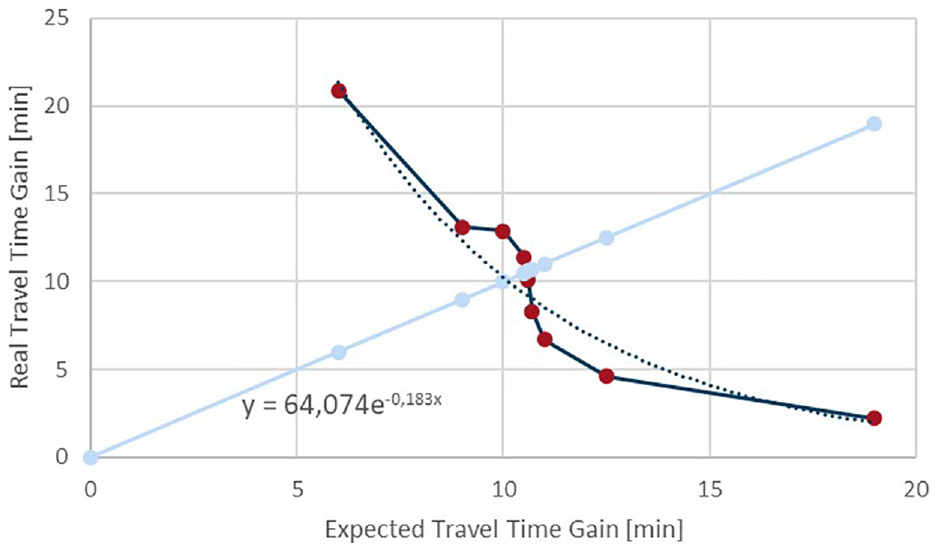
Ratio of expected travel time gain to real travel time gain for 0.5 €/km.

Conversely, a high expected travel time gain resulted in a high proportion of HOV and HOT vehicles, leading to high utilization of the managed lane, which significantly reduced achievable travel time gains. This effect can also be observed in reality when new managed lanes are implemented, and users initially assess whether this mode of mobility provides advantages for them. Over time, with knowledge, a habituation effect occurs; road traffic authorities could also intervene through variable toll rates. In this case, an optimum was reached, in which the expected travel time gain matched the real travel time gain at slightly more than 10 min of travel time. It is important to note that different curves can be observed for individual O-D pairs in Figure 2, and a uniform factor could not be directly applied to all O-D pairs for adjustment.

Table 2 presents travel time gains in minutes for different O-D pairs in the various scenarios. At first glance, it was evident that travel time gains were particularly significant for longer segments and high traffic volumes. However, for short distances, such as those involving only one exit, travel time gain can sometimes turn negative. These travel time losses typically amount to only a few seconds and, as explained, arise from the progress of privileged users merging into the managed occasionally being impeded rather than accelerated. In an individual opportunity assessment, some drivers may decide to stay on the regular lanes. This situation can lead to congestion caused by heavy traffic or substantial truck presence. However, it is important to note that these values are highly volatile and can occasionally yield positive results in individual simulation runs. Deviations of 100% or more are not uncommon in this analysis range.

As the traveled distances increased, so did the travel time gains, which tended to stabilize. The deviations decreased significantly with larger travel time gains, and for gains between 90 and 120 s, the values fluctuated by 20% to 30%. Once the threshold of 120 s of travel time gain was surpassed, the deviations decreased to single-digit percentages. The analysis highlighted the significant influence of traffic volume. In the section between Exit 4 and Interchange B, the traffic load was highest, and the freeway was partially congested. Here, travel time gains of up to 7 min could be realized over an approximate 5-km segment. Comparing the values, it became evident that merging into or exiting from the managed lane can lead to travel time losses of approximately 1 min.

Modal Shift and Modal Split

The following results are based on the modal split from Equations 1 to 4 and relate to the optimal values determined in Figure 2. Figure 3 illustrates how the proportion of vehicles using the HOT lane and the general-purpose lane (GPL) develop across different scenarios at system optimum. Here, HOVs, PT, and HOT vehicles (i.e., paying SOVs) can use the HOT lane, all vehicles can drive on the GPL, but nonpaying SOVs in particular must use it. It was evident that the share of HOT vehicles significantly decreased with increasing travel cost, whereas the share of HOVs increased. In addition, the optimal travel time savings per scenario were lower at higher costs. However, the fluctuations in this case were noticeably less pronounced. One possible explanation is that fewer individuals overall switched to HOV/HOT, resulting in fewer opportunities to interlace within the road network and access the desired travel lanes as the GPL became more heavily utilized.

Figure 3.

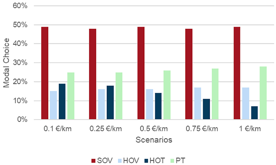
Modal split for vehicles entering at Intersection 1 and leaving at Intersection 6.

Figure 3 presents the modal split for the various scenarios. As the shift in modal split toward favoring PT and carpooling is a central political objective and the starting point for many managed lanes, we will now delve more deeply into this topic. In the following, we demonstrate the potential for shifting toward other transportation modes in the different systems.

Figure 4 illustrates the average modal split across the entire system and the various scenarios, including commuters who switched to PT instead of using the freeway for their commute. As road usage fees increased, there was a slight trend favoring PT and HOV at the expense of HOT. However, this trend was within a few percentage points, with the proportion of HOT vehicles being halved. As expected, the proportion of commuters willing to pay for a HOT lane decreased with higher costs. Nevertheless, it was evident that the overall influence of travel cost was quite limited. The proportion of SOVs remained almost constant across the different scenarios. This confirmed findings from our earlier research indicating that a significant portion of commuters prefer to stick with their SOV and are not willing to switch to HOVs, HOT vehicles, or PT ( 4 ). However, the small variations observed in the overall system were mainly because many vehicles only travel short distances on the freeway, creating insufficient incentive to switch from single-occupancy driving to other modes. The number of trucks in the system is not shown in detail as this remained constant across all scenarios, with a slight increase in their proportion to the total traffic resulting from the lower number of vehicles owing to carpooling and the shift to PT, which led to a decrease in the overall system.

Figure 4.

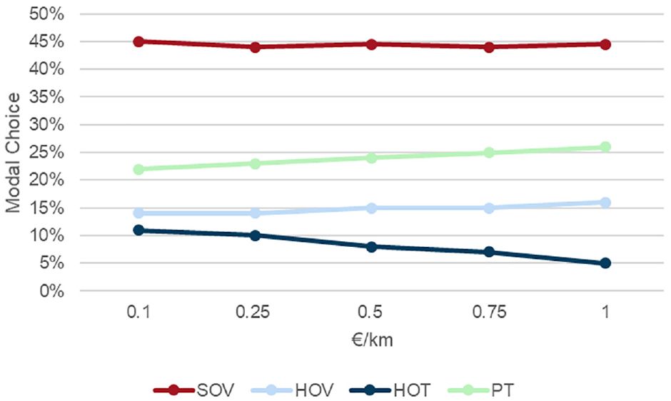
Modal split: whole network (weighted by route length).

In Figure 5, the average modal split across the entire system and the various scenarios is presented again, but this time it is adjusted to exclude trucks and PT. As road usage fees increased, a slight trend in favor of SOV and HOV at the expense of HOT became evident. However, this trend remained within a few percentage points. As expected, the proportion of commuters willing to pay for a HOT lane decreased with higher costs. Nevertheless, was again apparent that the overall influence of travel cost was rather limited. Overall, the analysis of the entire system clearly showed that in the optimal usage case, traffic was evenly distributed across the cross section.

Figure 5.

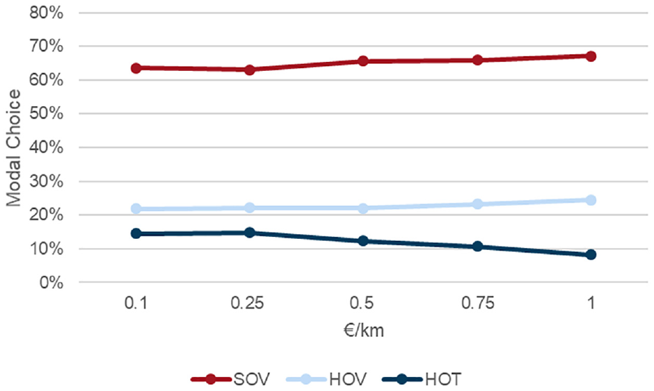
Private transport (without public transport [PT]): whole network modal split.

As a reminder, within this study, we considered a six-lane configuration with three lanes in each direction, including a managed lane (the left-hand lane). Consequently, two-thirds of the lanes were available for general-purpose use, which roughly corresponded to the distribution of vehicle type, with approximately two-thirds being SOV and a total of one-third being HOT vehicles and HOVs.

Comparing the results given, it was clear: on a short stretch of road, the price level did not have a significant influence on the commuters’ mode choice. The proportion of trucks in this example was the result of the random numbers used in the scenarios and served as a base load for the network; this would change with a different stretch of road, unlike the constant proportions of the other transportation modes. Overall, the values for SOV were significantly higher for short sections than those of the entire network, and there were slight increases for PT, whereas the other transportation modes showed weaker variations.

Travel Time and Travel Time Gain

The starting point for examining travel time gain was initially the travel times in the baseline scenario. In this scenario, there was no managed lane, and therefore no HOT vehicles that could purchase traffic-flow privileges. Consequently, only the groups SOV, HOV, and trucks were evaluated in this case, with HOVs and SOVs having no significant differences in their travel speeds. In subsequent evaluations, travel time refers to the SOVs of the base case.

Figure 6 compares the average travel times for the entire system between the baseline and alternative scenarios. The red line represents the average travel times of all vehicles in the network in minutes for the base case without a managed lane. SOV and HOV achieved the same travel times. For clarity, the SOV travel time is also indicated as the reference value for HOT vehicles. Comparing the different scenarios, it became evident that implementation of a managed lane led to an average travel time increase of a few seconds to 2 min for SOVs compared with the baseline scenario. In contrast, the situation improved for HOVs and HOT vehicles, with average travel time gains of up to 3 min. HOT vehicles were even slightly faster than HOVs, which can be attributed to the personal preferences of HOT drivers. For trucks, travel times worsened compared with the baseline owing to heavier congestion on regular lanes.

Figure 6.

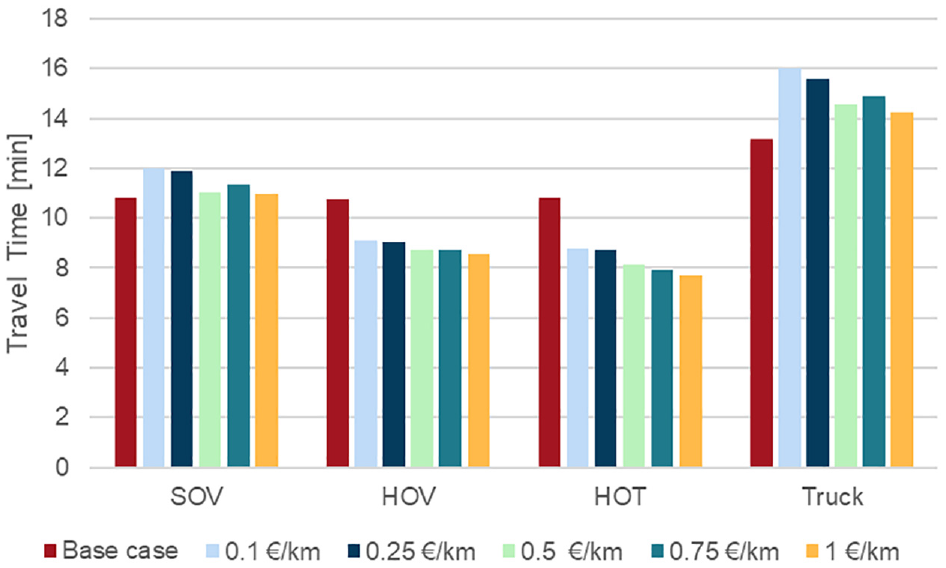
Travel time for the pricing scenarios: whole network.

With regard to the scenarios in general, it was interesting to note that the most favorable travel times for all types of vehicle occurred in the scenario with the highest costs. This was partly because, in this scenario, the most significant shift occurred toward PT, resulting in a reduction in the total number of cars in the network.

In contrast to Figure 6, which includes many vehicles that only traveled a short section on the freeway, thereby averaging out the travel time losses, Figure 7 shows the development of travel times for vehicles traveling from Interchange 1 to Interchange 6 in the different scenarios. This section was chosen to evaluate the effects of an extended journey on a managed lane that is not disrupted by entrance and exit processes. Here, significantly larger differences between the individual vehicle groups were apparent, with overall longer travel times. Once again, the red line represents the base case which serves as the reference without a managed lane. The five bars in the figure represent the different scenarios: travel time losses of up to 5 min compared with the reference scenario occurred, and HOT vehicles and HOVs were significantly faster than in the reference scenario. As observed in the overall system, trucks also experienced longer travel times in the presence of a managed lane.

Figure 7.

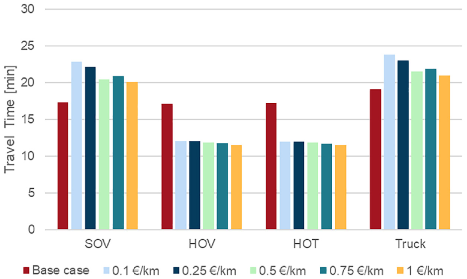
Travel time for the pricing: scenarios, Interchange 1 to 6.

Combining Figures 6 and 3 revealed that when considering all commuters, approximately half of the travelers experienced travel time losses compared with a freeway without a managed lane. When focusing solely on commuters who used the freeway, the ratio of beneficiaries to those experiencing losses was even more pronounced at one- to two-thirds. Examining the section between the two junctions, 1 and 6, which corresponded to a combination of Figures 7 and 3, yielded a very similar distribution of beneficiaries and losers from a managed lane. In general, the situation tended to worsen for commuters who traveled only a short distance on the freeway, as they were less likely to join a carpool or pay to use a HOT lane owing to their relatively lower potential travel time gain resulting from the shorter distance. For instance, only one in five commuters benefited from the managed lane on a trip between Interchanges 2 and 3.

Figure 8 depicts the percentage of traffic participants experiencing travel time gains and losses. Negative values on the axes indicate that vehicles were faster than in the baseline scenario, whereas positive values imply longer travel times. In this analysis, we focused on vehicles that entered at either A or 1 and then traveled the entire route up to 6 or B. Participants who exited earlier or entered later were not initially considered. Furthermore, all participants using PT were excluded since there was no clear correlation between the scenarios and faster or slower travel times. Examining the graph, for the scenario with a cost of 0.1 €/km, nearly 85% of the SOVs experienced longer travel times compared with the baseline scenario, whereas approximately 15% were faster. This proportion shifted in favor of those who were faster than the baseline scenario as the prices per kilometer increased, reaching 68% for 1.0 €/km. A similar pattern was observed for the trucks, with slightly different percentage shares. Over 80% of them experienced longer travel times without the managed lane, and this percentage decreased with higher costs. In contrast, the HOT vehicles and HOVs exhibited different behavior. Except for a few vehicles, these groups were always faster when using the managed lane, consistently achieving values of 99% to 100% for the proportion of faster vehicles.

Figure 8.

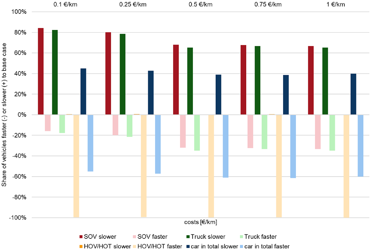
Share of vehicles being faster (−) or slower (+) compared with the base case.

Figure 9 presents the average travel times in the analyzed section, based on Figure 6. For the sake of readability, HOT vehicles and HOVs are combined in the graphs, as they exhibited nearly identical patterns. The values at 0 €/km reflect those of the baseline scenario, in which no managed lane exists. This further illustrated the shift in travel times. The evaluation revealed a general tendency of decreasing average travel times, with a temporary increase occurring in the range between 0.6 and 0.8 €/km. This was also evident in the average speed and all other analyses. Overall, as mentioned earlier, the travel times for SOVs and trucks were higher than those of the baseline scenario, whereas travel times for HOVs and HOT vehicles were lower. This analysis will be of greater significance, particularly in the evaluation of emissions in the following section.

Figure 9.

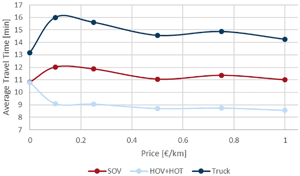
Average travel time.

Emissions

As with the simulations of individual trajectories, Aimsun was used to determine the emissions. During the Euro Working Group on Transportation Conference 2023, we presented an initial paper on the topic of CO₂ emissions on freeways ( 16 ). We will delve further into the field of emissions in this and subsequent papers. In the present paper, we limit our investigation to two types of emissions, namely CO₂ and NOx. For this purpose, we utilized the London Emission Model ( 17 – 20 ), which has been integrated into the Aimsun Next software as an extension. The emissions classes were chosen based on statistics from the German Federal Statistical Office ( 21 ).

In addition to optimizing traffic flow and -control, emissions reduction is a central tenet of managed lanes. Figure 10 illustrates the CO₂ emissions during the peak hour for the entire network under different scenarios. It is evident from the graph that CO₂ emissions decreased with increasing toll costs. The only exception was observed around the 0.75 €/km toll value, where CO₂ emissions briefly increased for a short section. To reference this increase in values and to rule out the possibility of it being an erroneous result in the analyses, we densified the calculation points in this range and proceeded in increments of 0.05 €/km. This densification of values confirmed the observed increase, which was then followed by a steady decline in the values. Overall, however, the emissions decreased by around 2 tons of CO₂ per hour during the peak hour. These savings can be attributed to two effects: first, a lower number of vehicles results in reduced emissions, and second, traffic flow becomes smoother, leading to a reduction in fuel consumption and, consequently, emissions, owing to the reduction in acceleration and braking events. The noticeable increase at 0.75 €/km also aligned with the temporary increase in SOV traffic, as described earlier. Therefore, the data from this study were consistent, even though further investigation is required to pinpoint the exact cause. Initial insights into this issue were mentioned in the preceding section. In Figure 9, the average travel times for the different scenarios are also presented. Here, we observed an increase in travel time in the range between 0.6 and 0.8 €/km, similar to that observed for CO₂ emissions and as will be seen for NOx emissions as well.

Figure 10.

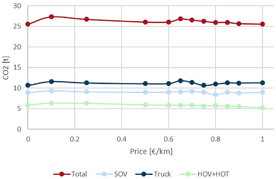
CO₂ emissions.

However, it is essential to compare these results with the baseline scenario. In the baseline scenario, CO₂ emissions amounted to approximately 25.5 tons per peak hour, which was lower than all the scenarios considered. Only the 1.0 €/km toll scenario showed similar values. The reasons for this lie in the much more frequent acceleration and stop events resulting from the significantly denser traffic on the two GPLs.

The second pollutant group we examined in this study was NOx. The trend of NOx emissions across the different scenarios is depicted in Figure 11. The patterns are similar to those of CO₂ emissions, with values dropping more sharply at the beginning and more slowly toward the end. However, in the case of NOx values, the increase in the 0.75 €/km scenario was even more pronounced. Comparing the results of each scenario with the values of the base case, the importance of a stable and homogeneous traffic flow became even more evident. In the baseline scenario, during peak hours, just under 50 kg of NOx was emitted per hour, which was 3.2 kg less than in the most favorable scenario. In contrast, compared with the baseline scenario, the least favorable case saw an increase of nearly 10 kg of NOx per hour, representing an approximate 20% rise.

Figure 11.

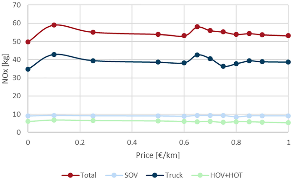
NOx emissions.

In Figure 12, the CO₂ emissions per vehicle group and kilometer are presented. At this point, trucks were omitted as their emissions were eight times higher than the other vehicle groups, making the figure significantly harder to read. Therefore, it is essential to consider that even the total emissions of the three vehicle groups depicted here were lower than the CO₂ emissions from heavy-duty trucks. As the values of heavy-duty vehicles were significantly higher than those of cars, the heavy-duty traffic is represented in the diagram as bars rather than as a line graph, and has its own axis with corresponding units. In general, the values were about five times higher. The results showed that the emissions of different vehicle types that were car-based were very close together, differing only by a few grams per kilometer, whereas there were slightly larger deviations for the trucks. These findings corresponded with those from Figure 9. As is widely known, lower travel speeds lead to lower emissions, which was also evident in this analysis. Areas with lower speeds exhibited the lowest emissions. Furthermore, it was observed that as the managed lane became more freely available at higher costs per kilometer, the consumption for the relatively faster-moving HOT vehicles increased. In the case of SOVs, there was a clearly discernible homogenization and partial acceleration of traffic over the course of the scenarios. Presentation of NOx values per vehicle is omitted in the following analyses because the curves followed an almost identical pattern. In both cases, the emissions of heavy-duty trucks dominated the overall emissions, whereas the speed profiles of the SOVs, HOVs, and HOT vehicles were easily distinguishable.

Figure 12.

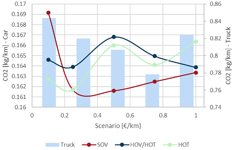
CO₂ emissions per vehicle and kilometer.

Summary of Scenarios

When comparing the different scenarios, the following results became apparent. The average travel times in the base scenario were below those of all the considered cost scenarios. Specifically, for users of the GPL, travel times decreased substantially with increasing costs, up to a reduction of 20%, whereas for the HOT lane, only a very slight trend was noticeable. This trend became more pronounced with increasing route length. The variation in CO₂ emissions was minimal but tended to be higher than those in the base scenario. However, these fluctuations were slight, keeping the emissions at a consistent level. The situation was different for NOx emissions, which consistently exceeded those of the base scenario in the various managed lane scenarios.

Interpretation

The present study has demonstrated that HOT lanes in Germany have a certain potential to shift traffic toward carpooling and PT. It was evident that commuters need to travel a certain distance on the managed lane for the incentives to take effect. This, in part, was because of the gradual buildup of travel time savings. For instance, when traveling at 60 km/h on the GPL and 100 km/h on the managed lane, approximately 12 km are needed to achieve a travel time advantage of 5 min. If the GPL speed increases to 80 km/h and the managed lane speed rises to 120 km/h, 20 km are required to gain a 5-min travel time advantage. Only when the speeds on the GPL decrease to an average of 50 km/h or less because of congestion, can sufficiently large travel time savings be achieved even on shorter distances. However, this condition results in significantly higher emissions, making it undesirable, just to highlight the benefits of the managed lane, to artificially restrict capacities to the extent that congestion and slow-moving traffic occur.

When evaluating HOT lanes, the entire system must always be considered. Most commuters using the freeway for their daily commute cover a distance of 10 to 15 km on the freeway. However, there is also a considerable baseline traffic volume, consisting of vehicles that travel longer distances, which only pass through the section under consideration, regardless of whether they are cars or trucks. For these vehicles, which form part of the general motorized individual traffic, there is little potential for pooling or switching to PT, as they are usually not commuters. The higher the proportion of these vehicles, the lower the potential of a HOT lane in such a section of roadway. In such cases, other managed lane systems may be more effective ( 13 , 22 ), such as temporary shoulder lanes or dynamic signage that guides traffic in a larger context.

Before implementing a managed lane, in this case a HOT lane, the objectives and conditions of this measure must be clear. Should the system be optimized for environmental impacts or travel time? What are the effects on neighboring sections? As this study has shown, individual objectives can sometimes contradict each other, for example, when pollutant emissions increase significantly as a result of denser traffic, while travel times decrease for privileged vehicles. A balanced optimum for all aspects needs to be found, which should be maintained through continuous intelligent control.

The investigation revealed that pricing can achieve a certain control effect. As expected, low toll costs per kilometer incentivized larger groups of commuters to switch to the HOT lane. This comes at the expense of PT and carpooling. Conversely, with increasing costs, the attractiveness of carpooling and PT, as well as the willingness to accept travel time losses on the GPL, increased. In general, the managed lane demonstrated clear speed advantages over the GPL, as described earlier, but these advantages were fully effective only on longer stretches. HOT users tended to exhibit higher speeds compared with HOVs. This could be attributed to the willingness of people who spend money for an accelerated trip to maximize their investment in the form of maximum travel time savings. Moreover, people may be especially inclined to use the HOT lane when, for example, they are on a tight schedule and urgently need to reach an appointment. In contrast, HOV drivers may be more conscious of their responsibility for the occupants in their vehicles, leading to a more balanced driving style. However, owing to the shared use of the managed lane, the actual travel time difference between HOV and HOT vehicles was minimal. This would change if two lanes were designated as managed lanes, allowing for overtaking opportunities.

Conclusion

Considering the results presented in this paper, it can be concluded that HOT lanes have potential but are not a one-size-fits-all solution. In areas with high traffic congestion and low speeds, HOT lanes provide an incentive for switching to carpooling or PT. However, this can lead to displacement effects on adjacent road networks and increased emissions.

Before implementing a managed lane, a thorough examination is necessary to determine whether it can effectively demonstrate its strengths in the selected road section. It is crucial to avoid excessive through traffic compared with vehicles entering and exiting the section. Moreover, a careful assessment is required to ensure that the elimination of a lane does not lead to additional problems, particularly in relation to emissions.

Analysis of the scenarios demonstrated that very low toll rates for using the HOT lane can have negative impacts on the modal split of HOVs and PT. An automated, intelligent management system is necessary to optimize HOT lane utilization, ensuring that capacities are not wasted and at the same time do not jeopardize the goal of strengthening HOVs and PT.

When introducing a managed lane, the consequences must be carefully weighed. In the context of this paper, we have demonstrated that, typically, 50% or more of the commuters experience worsened travel times. Factors such as congestion on the route, average travel distance in the affected section, and the available alternatives play a crucial role in this assessment.

Another insight from this study is the significant influence of homogeneous traffic on emissions. Even displacing a four-digit number of vehicles to HOVs and PT did not offset the higher emissions resulting from acceleration and deceleration processes. An additional intelligent traffic control system, particularly focusing on optimizing speeds, could potentially address this issue.

Overall, HOT lanes, taking into account successful examples from other countries, exhibited good potential for improving the traffic situation in Germany. However, legal considerations in Germany need to be clarified, as tolls are not currently imposed on freeways, and this is not legally feasible. Nevertheless, the laws have been prepared accordingly and could be modified.

In the next steps, the authors plan to pursue multiple lines of action, to be included in various publications. Firstly, the findings of this paper will be applied to a real network, and simulations will be used to assess the impacts on an existing road network. The authors will additionally delve into the environmental effects of managed lanes in general and HOT lanes in particular. Suitable parameters will be identified, and their impacts will be quantified. Furthermore, the anomalies observed in the scenarios with a toll rate of 0.75 €/km will be thoroughly investigated to provide a comprehensive explanation for their occurrence. Lastly, the authors plan to extend the examination from the peak hour to cover an entire day.

Footnotes

Acknowledgements

The authors thank the Free State of Bavaria and the Bavarian Ministry of Housing, Construction, and Transport for the opportunity to conduct research on managed lanes in general and HOT lanes in particular during a secondment to the Technical University of Munich.

Author Contributions

The authors confirm contribution to the paper as follows: study conception and design: T. Schoenhofer, B. Kaltenhaeuser, K. Bogenberger; data collection: T. Schoenhofer, B. Kaltenhaeuser; analysis and interpretation of results: T. Schoenhofer, B. Kaltenhaeuser; draft manuscript preparation: T. Schoenhofer, B. Kaltenhaeuser, K. Bogenberger. All authors reviewed the results and approved the final version of the manuscript.

Declaration of Conflicting Interests

The authors declared no potential conflicts of interest with respect to the research, authorship, and/or publication of this article.

Funding

The authors received no financial support for the research, authorship, and/or publication of this article.

ORCID iDs

Thomas Schönhofer

Bernd Kaltenhäuser

Klaus Bogenberger

References

Schönhofer

Bogenberger

A Comprehensive Review on Managed Lanes in Europe. In TRB, Washington, D.C., 2022.

Weyland

Buck

H. S.

Vortisch

Zeidler

Analysis of the Effects of an HOV Lane on a German Freeway – A Simulation Study with PTV VISSIM. TRB 98th Annual Meeting Compendium of Papers. Ed.: Transportation Research Board, Washington, DC, 2019.

Chang

Wiegmann

Smith

Bilotto

HOV Lanes Emerged in Areas Across the Country for a Variety of Reasons, 12/2008. https://ops.fhwa.dot.gov/publications/fhwahop09029/fhwahop09029.pdf. Accessed July 11, 2023.

Schönhofer

Kaltenhäuser

Bogenberger

Analysis of Survey Data on Preferences of German Commuters Using Structural Equation Modeling. In TRB, Washington, D.C., 2023.

Fontes

Fernandes

Rodrigues

Bandeira

J. M.

Pereira

S. R.

Khattak

A. J.

Coelho

M. C.

Are HOV/eco-Lanes a Sustainable Option to Reducing Emissions in a Medium-Sized European City?

Transportation Research Part A: Policy and Practice, Vol. 63, 2014, pp. 93–106.

Borup

Geerken

, eds. System Innovation for Sustainability 2. Case Studies in Sustainable Consumption and Production – Mobility. Taylor and Francis, London, 2017.

Schijns

Eng

High Occupancy Vehicle Lanes – Worldwide Lessons for European Practitioners. Urban Transport XII: Urban Transport and the Environment in the 21st Century, Prague, Czech Republic, July 12–14, 2006, WIT Press, Southampton, UK, pp. 181–193.

Simonsen

Sandelien

The First Norwegian Carpool Lane Opened in Trondheim. Nordic Road & Transport Research Vol. 13, No. 3, 2001.

University of Michigan. Personal Transportation Factsheet CSS01-07, Center for Sustainable Systems, 2022.

10.

Eck

Öffentliche Infrastrukturinvestitionen. Entwicklung, Bestimmungfaktoren Und Wachstumswirkungen. Ifo-Inst. f. Wirtschaftsforsch, München, 2015.

11.

Schönhofer

Kaltenhäuser

Bogenberger

Potentials for Modal Shift Through HOV/HOT Lanes in Germany. 4th International Symposium on Freeway and Tollway Operations, Vienna, Austria, June 26–30, 2023.

12.

Handbuch Für Die Bemessung Von Straßenverkehrsanlagen. HBS 2015, FGSV FGSV 299 B, Forschungsgesellschaft für Straßen- und Verkehrswesen, 2015.

13.

Collier

Goodin

MANAGED LANES: A Cross-Cutting Study, 2004. https://ops.fhwa.dot.gov/freewaymgmt/publications/managed_lanes/crosscuttingstudy/index.htm. Accessed July 21, 2023.

14.

Statista. Verkehr in Deutschland – Fahrleistung Von Pkw Bis 2021 and Statista. https://de.statista.com/statistik/daten/studie/2984/umfrage/entwicklung-der-fahrleistung-von-pkw/. Accessed July 11, 2023.

15.

Hinweise Zur Mikroskopischen Verkehrsflusssimulation. Grundlagen Und Anwendungen, Forschung Straßenbau und Straßenverkehrstechnik FGSV-388, Forschungsgesellschaft für Straßen- und Verkehrswesen, 2006.

16.

Wang

Kaltenhäuser

Schönhofer

Bogenberger

Leonhardt

Simulation-Based Estimation of CO₂ Emissions Per Vehicle by Reducing Traffic Volumes During Morning Peak Hours on Highways. In EWGT, Santander, 2023.

17.

Triantafyllos

Illera

Djukic

Casas

Dynamic Congestion Toll Pricing Strategies to Evaluate the Potential of Route-Demand Diversion on Toll Facilities. Transportation Research Procedia, Vol. 41, 2019, pp. 731–740.

18.

Graham

D. J.

Stettler

M. E. J.

Has the Ultra Low Emission Zone in London Improved Air Quality?

Environmental Research Letters, Vol. 16, No. 12, 2021, p. 124001.

19.

Aimsun. Environmental Models – Aimsun Next Users Manual. https://docs.aimsun.com/next/22.0.2/UsersManual/EnvironmentalModels.html#london-emission-model-lem. Accessed July 20, 2023.

20.

EarthSense. Smart City Solutions Through Combined Air Pollution and Traffic Technologies. https://www.earthsense.co.uk/post/nevfma-combined-airquality-traffic-technologies. Accessed July 20, 2023.

21.

Statista. Pkw-Bestand Nach Emissionsklassen 2023 | Statista. https://de.statista.com/statistik/daten/studie/6701/umfrage/gemeldete-pkw-je-emissionsklasse/. Accessed July 20, 2023.

22.

Fitzpatrick

Brewer

M. A.

Chrysler

Wood

Kuhn

Goodin

Ungemah

Perez

Dewey

Thompson

Swenson

Henderson

Guidelines for Implementing Managed Lanes. Transportation Research Board, Washington, D.C., 2016.

Simulation Approach to Estimate the Potential of High-Occupancy Toll Lanes on German Freeways

Abstract

Keywords

Motivation

Data and Traffic Model

Scenarios and Modeling

Results, Benefits, and Impacts

Modal Shift and Modal Split

Travel Time and Travel Time Gain

Emissions

Summary of Scenarios

Interpretation

Conclusion

Footnotes

Acknowledgements

Author Contributions

Declaration of Conflicting Interests

Funding

ORCID iDs

References