Sage Journals: Discover world-class research

Abstract

High-occupancy vehicle (HOV) lane performance degradation has become more prevalent in many regions because of the growing travel demand and the increasing number of HOV lane-eligible vehicles. Conventional capacity expansion strategies, such as adding a second HOV lane, can be a promising solution. However, they can be difficult in areas where there is little room left to add new travel lanes in both directions. In that case, adding a contraflow HOV lane could be a good compromise, especially if the peak travel demands in the HOV lanes are tidal. In this work, we study the impact of adding a contraflow HOV lane on a section of the I-215 freeway, which connects two major cities in Riverside County, California. Two alternative designs, “full contraflow” and “partial contraflow” HOV lanes, are evaluated in the traffic microsimulation environment. The evaluation results show that in the case of the full contraflow HOV lane design, the average delay during peak hours in the southbound direction of the freeway would be reduced by 76% compared with the scenario with no additional HOV lane. The implementation of the full contraflow HOV lane to supplement the existing HOV lanes would also increase the average speed in the currently degraded HOV lane from 37.8 to 55.0 mph, which is significantly above 45 mph, the speed threshold for HOV lane performance degradation.

Keywords

operations managed lanes congestion management high-occupancy vehicle lanes traffic simulation microscopic traffic simulation

High-occupancy vehicle (HOV) lanes have been used as a tool to manage traffic congestion and improve travel time reliability on freeways for decades, and most HOV lanes have been effective at providing travel time savings for eligible vehicles. However, because of the growth in travel demand and the number of HOV lane-eligible vehicles, many HOV lanes in the U.S.A. have become congested with degraded performance. For example, according to the 2019 California High Occupancy Vehicle Facilities Degradation Report and Action Plan, 26% and 40% of the 1302 HOV lane-miles monitored were degraded in the morning and afternoon peak hour periods, respectively ( 1 ). Not only is the number of degraded HOV facilities in California increasing, but the level of degradation is also getting more severe each year. According to the California Department of Transportation (Caltrans) ( 1 ), compared to the previous year, the 2019 HOV degradation rate increased 6% and 9% in the morning and afternoon peak hours, respectively, with approximately 46% of the degraded facilities in the afternoon peak hour experiencing extreme levels of degradation (degradation occurs 75% or more of the time). In 2020, the HOV degradation rate dropped by a large margin because of the pandemic, but it has been increasing again since June 2020 and has reached a similar level to that in 2019.

To address the HOV lane performance degradation issue, several strategies have been proposed, which can be grouped into four categories—capacity expansion, operational improvement, education, and enforcement. Operational improvement strategies, such as increasing vehicle occupancy requirements or converting HOV lanes to high-occupancy toll (HOT) lanes, have high potential to address the degradation issue, but these strategies may unintentionally affect the travel speed of the vehicles in the mixed flow (MF) lanes. Education and enforcement strategies, such as increasing public awareness and installing additional signage along the HOV lanes, could be implemented at a low cost, but these strategies are only applicable to HOV facilities with high violation rates. For HOV facilities with many HOV lane-eligible vehicles, capacity expansion strategies, such as adding a second HOV lane, could be an effective way to alleviate the HOV lane performance degradation. However, such strategies can be difficult in some areas where there is little room left to add new travel lanes in both directions. In that case, adding a new HOV lane that operates in a contraflow or reversible fashion could be a good compromise, especially if the peak travel demands in the HOV lanes are tidal, that is, morning peak in one direction and afternoon peak in the other direction.

The idea of using contraflow or reversible lanes for capacity expansion and congestion mitigation has been proposed earlier, and researchers have studied the impact of such a design. A reversible lane is a barrier-separated facility in the median with one or more lanes that operates in one direction during the morning peak period and in the other direction during the afternoon peak period. Compared to the reversible lane, the contraflow lane operates under the same principle but uses movable barriers to manage the direction of travel. Skowronek et al. ( 2 ) investigate the operational effectiveness of Dallas’ HOV lane, in which a barrier-separated reversible lane is evaluated and monitored for performance. Zhao et al. ( 3 ) propose a contraflow left-turn pocket lane design to mitigate congestion caused by heavy left-turn demand, and show that it can increase a signalized intersection’s throughput and decrease the intersection’s average delay. Wolshon and Lambert ( 4 ) study the impacts of reversible lanes on safety, operations, and the environment, and give suggestions on their design and implementation requirements. Waleczek et al. ( 5 ) discuss the effects on traffic flow and road safety of a reversible lane system in a work zone in Germany. Using the recorded traffic data, the authors conclude that the reversible lane system is a useful and safe tool for freeway work zones with high fluctuation in the peak traffic flow direction. Zhao et al. ( 6 ) develop a lane-based optimization model to guide the integrated design of reversible lanes on an urban arterial to maximize the overall operational performance.

In addition, researchers have also studied the adaptive operation of reversible and contraflow lanes. Zhou et al. ( 7 ) and Mao et al. ( 8 ) develop a real-time dynamic reversible lane scheme in which lane change control models are applied based on the collected traffic information. In Meng and Khoo ( 9 ), a genetic algorithm that is embedded in a microscopic traffic simulation module, as well as a string repairing procedure to find the optimal contraflow scheduling solution, is developed. In Pérez-Méndez et al. ( 10 ), an adaptive reversible lane model is proposed using cellular automata, so that reversible lanes can change their direction using real-time information to respond to traffic demand fluctuations. Although it can significantly reduce the average delay, the adaptive reversible lane model is complex and difficult to implement.

The previous works reviewed above primarily study the impact or the operation of existing reversible and contraflow lanes, and most are focused on studying reversible lanes. The use of a contraflow HOV lane as a strategy to mitigate HOV lane performance degradation and the impact of different contraflow HOV lane designs on the potential improvements in traffic throughput and traffic speed have not been investigated before. Because of the higher costs of constructing and operating a contraflow HOV lane as compared to a concurrent HOV lane, it is important to conduct a thorough evaluation, such as with microsimulation, of the potential operational improvements of this strategy before field implementation.

In this work, the study site is a section of Interstate 215 (I-215) in Riverside County, California, where there is already one HOV lane in each direction. This freeway section has experienced a significant increase in both the overall travel demand and the number of HOV lane-eligible vehicles. As can be seen from Figure 1, the mean afternoon congestion duration (green line with cross marker) in the HOV lane of I-215 southbound has been gradually increasing since 2015, exceeding 200 min per day on many occasions. A vast drop in congestion duration occurred during the COVID-19 pandemic. However, after a period of light congestion, this section of the HOV lane has experienced heavy congestion again, and a plan for mitigating the lane performance degradation is needed.

Figure 1.

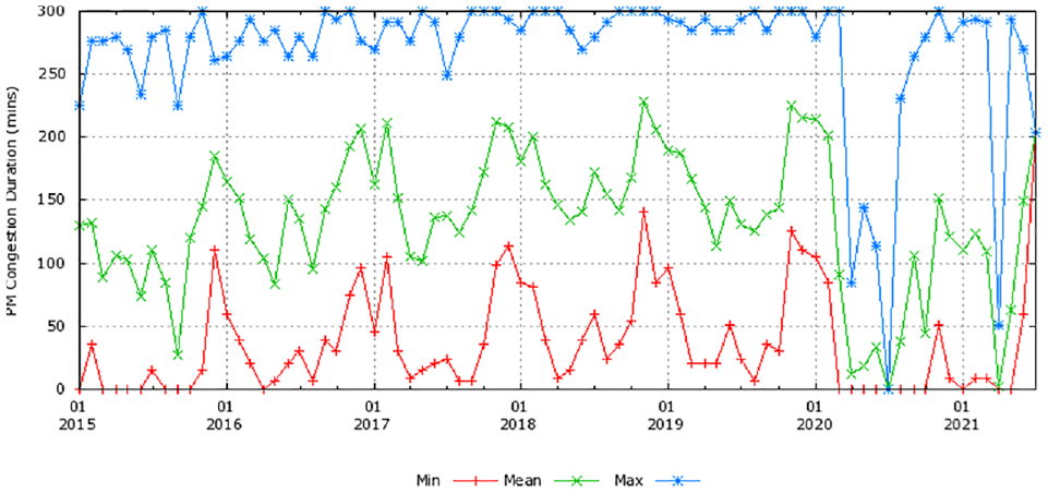
Afternoon congestion duration (speed < 35 mph) in the high-occupancy vehicle lane of I-215 SB in Riverside County, California, on weekdays since 2015. (Color online only.)

While freeway operations techniques such as ramp metering could lead to traffic flow improvements on the freeway, those techniques are primarily designed to improve traffic flow in MF lanes. To address the HOV lane performance degradation issue, additional measures that directly mitigate congestion in HOV lanes are needed. Because of the study site already having an existing HOV lane in each direction with limited space in the median, we considered adding a contraflow HOV lane instead of a reversible HOV lane. We evaluated two designs of contraflow HOV lanes. Besides the classic contraflow design where the entire length of the new HOV lane is directional according to the tidal peak travel demands, we also evaluated a mixed design in which part of the new HOV lane is one direction only while the remainder is directional. By building and calibrating the microsimulation networks of the two designs, the potential traffic speed improvement of each design could be assessed. The results can then be used to guide the selection of a design for field implementation.

The remainder of this paper is organized as follows. Firstly, we describe the simulation-based evaluation methodology, including study site selection, simulation network coding, and network calibration and validation. Then, we present the simulation results with respect to performance metrics of the different HOV lane designs. Lastly, we conclude the paper and discuss future work.

Methodology

We conducted the evaluation of contraflow lane designs for HOV facilities using Vissim ( 11 ) microsimulation software. Firstly, we selected a study site and built its microsimulation network based on real-world geographic images. Then, we calibrated and validated this baseline network using traffic data from Caltrans’s Performance Measurement System (PeMS) ( 12 ), which provided historical and real-time traffic data collected from over 39,000 individual detectors on California’s freeways. In addition to the baseline network, we also developed two additional microsimulation networks representing two different designs for adding a new HOV lane at the study site. All these steps are described in the following sections.

Study Site Selection

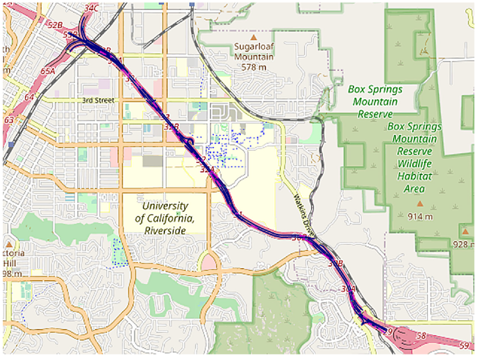
Since this study is focused on mitigating congestion in HOV facilities, the study site was selected among the HOV facilities that are under major degradation. Based on the 2019 California High-Occupancy Vehicles Facilities Degradation Report and Action Plan ( 1 ) and discussion with Caltrans staff, we selected the HOV facilities on I-215 (between absolute post miles [PMs] 30 and 35) in Riverside County, as shown in Figure 2, as the study site.

Figure 2.

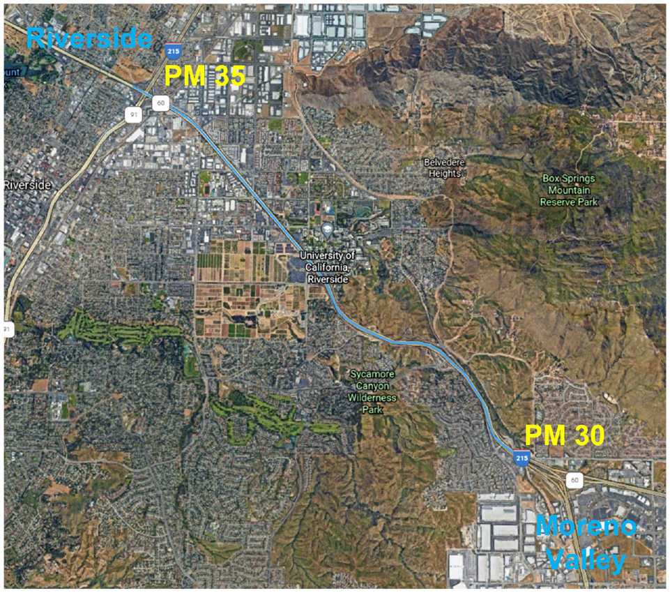
Selected high-occupancy vehicle facilities for study.

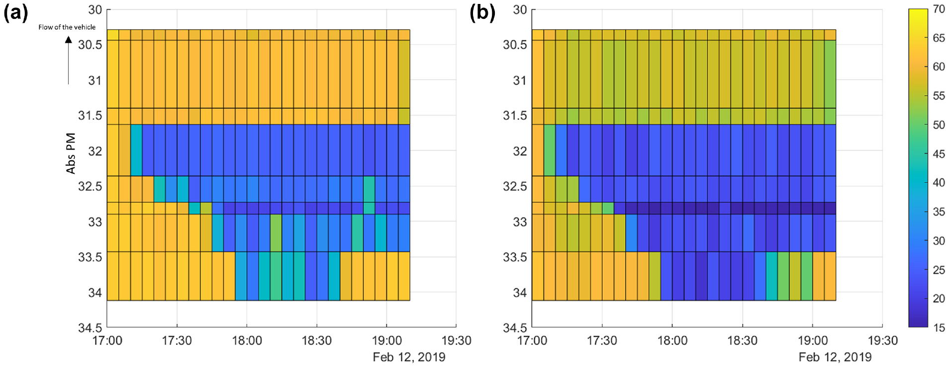
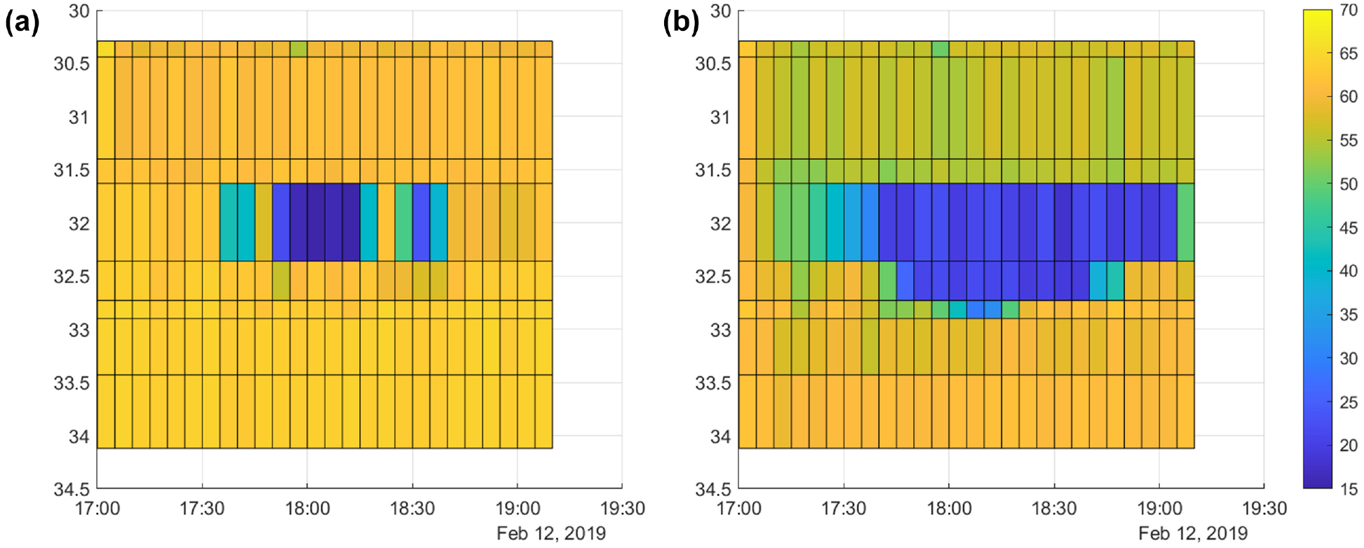
The selected freeway segment connects two major cities in Riverside County, the City of Riverside (top left-hand corner) and the City of Moreno Valley (lower right-hand corner). The two cities are the top two most populous cities in Riverside County with an elevation difference of 180 m. Because of the large amount of transport of goods and people, the segment is usually heavily congested during both morning and afternoon peak periods. According to the 2019 Degradation Report, the HOV facilities in both directions of this freeway section are extremely degraded, the highest level of degradation status. To further understand the congestion patterns on the freeway section, we checked the PeMS ( 12 ), which provides visualization of the typical traffic speed on any chosen days of week as estimated from historical traffic data, as shown in Figure 3.

Figure 3.

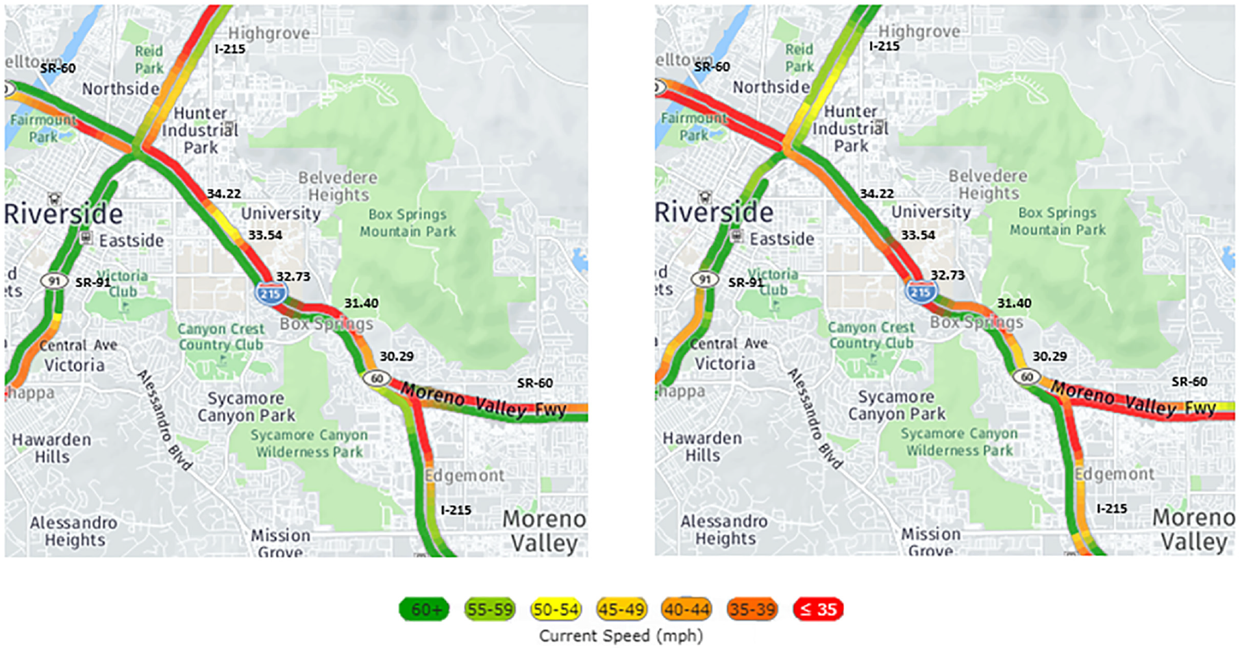
Typical traffic during morning peak (a) and afternoon peak (b) speed on Tuesdays. The absolute post mile (PM) is labeled next to the speed map according to the California Department of Transportation postmiling system.

As shown in Figure 3, on a typical Tuesday the morning and afternoon peak hours are usually at around 8 a.m. and 6 p.m., respectively. During the morning peak, heavy traffic congestion occurs at both the north and south portion of the northbound, near the interchange of SR-60 and I-215 in the City of Moreno Valley (absolute PM 30.29) and the interchange of SR-60 and SR-91 in the City of Riverside (absolute PM 34.22). In the afternoon peak, congestion occurs at the north end of the southbound and affects the north portion of the southbound direction. It is gradually relieved along the southbound direction. In the southbound direction, there is also moderate congestion in the south portion of the section.

This pattern of congestion indicates that the majority of the vehicles travel northbound in the morning and southbound in the afternoon, which supports our idea to add a new contraflow HOV lane in the median to increase the capacity of the existing HOV lanes in both travel directions. Also, as shown from the bird’s-eye view of the existing facility and the street view of both directions in Figure 4, there is enough space to add a single HOV lane in the middle with the graphical cross-section design, as shown in Figure 4d. The new HOV lane consists of a 3.7 m contraflow lane and two 1.2 m shoulders. However, the length of the new HOV lane that should be operated in a contraflow fashion needs to be determined. Specifically, we evaluated two possible configurations for the new HOV lane.

Full contraflow (FC) HOV lane: this configuration adds a new contraflow HOV lane along the entire section. This means that the new HOV lane is open to northbound traffic during the morning peak hours and to southbound traffic during the afternoon peak hours.

Partial contraflow (PC) HOV lane: this configuration adds a new HOV lane along the entire section, but operates it as a contraflow HOV lane only in the north portion of the section. This means that the north portion of the new HOV lane is operated as a contraflow lane in the same way as the previous configuration. On the other hand, the south portion is always used for northbound traffic, essentially forming dual HOV lanes in that direction. The main reason for this configuration is that in the south portion of the study section, the northbound traffic always appears to be more congested than the southbound traffic.

Figure 4.

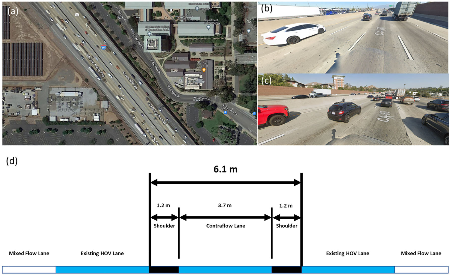
Existing facility (a) and street view of both directions (b), (c) with graphical cross-sections (d) of the proposed scenarios.

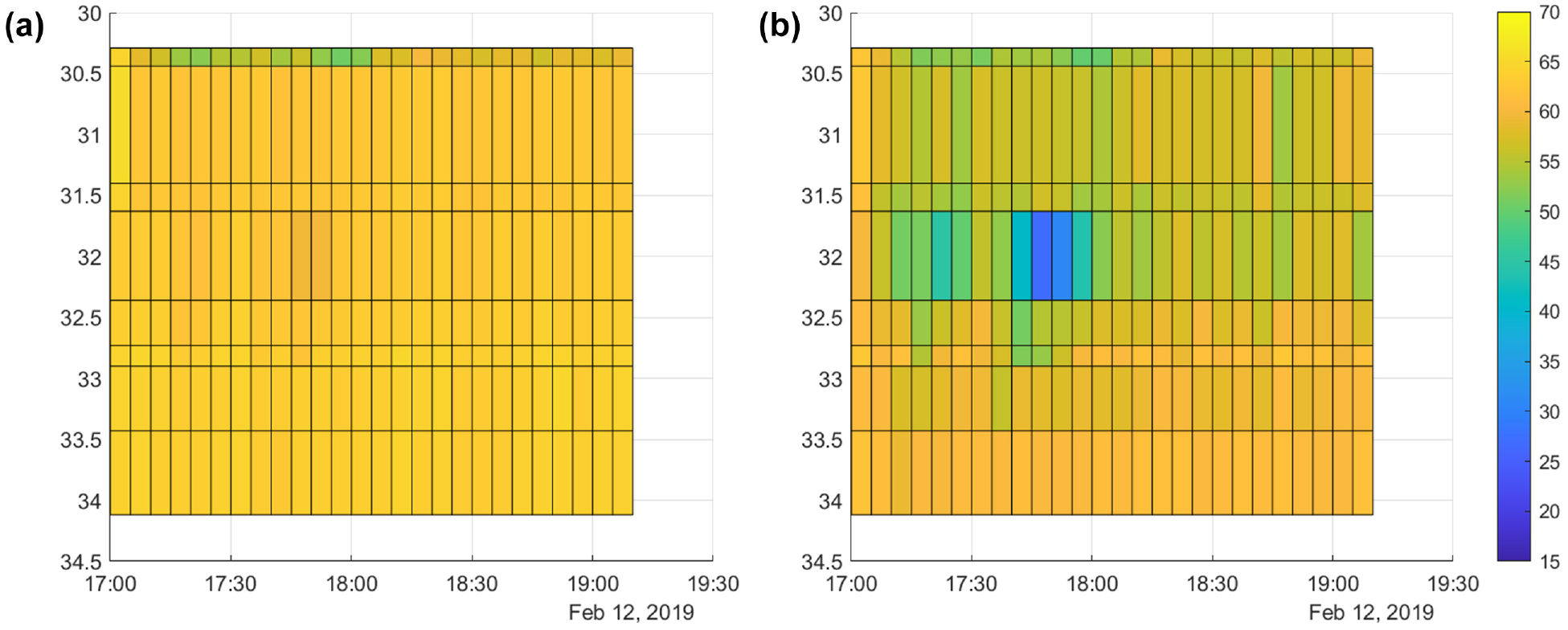
Once the study section had been selected, the research team checked the reliability of the traffic data reported by the PeMS from 2018 to 2019 based on the recorded detector health information. We found that during February 2019 the detectors on the freeway section were healthy for over 90% of the time. We then examined the average traffic volume at 5-min intervals and found the period from 5:35 to 6:35 p.m. to have the highest volume. Thus, we selected Tuesday 12 February 2019 as the target day of study for the simulation modeling. To validate the selected chosen period, we checked the vehicle miles traveled (VMT) and vehicle miles weighted speed (Q) from the PeMS, as shown in Figure 5.

Figure 5.

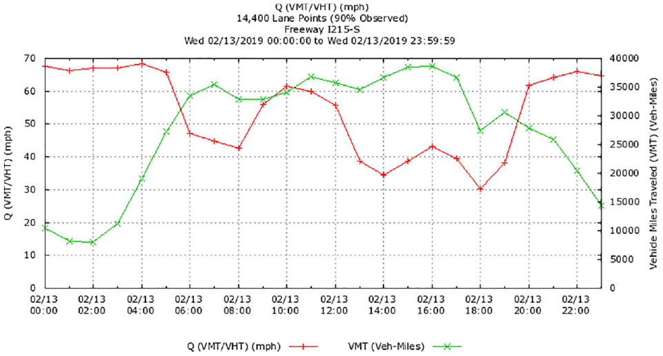
Vehicle miles traveled (VMT) and Q plot for I-215 south between absolute post miles 30 and 35. The weighted speed is lowest at 6 p.m. when congested.

Simulation Network Coding

Figure 2 shows the 5-mi freeway section of the study site. The section has three inflow sources from the north end, which are SR-60 eastbound, I-215 southbound, and CA-91 eastbound. The number of lanes on different segments of the study site varies from four to six, with the leftmost lane a full-time HOV lane. The elevation difference between the north end and the south end of the section is 180 m. There are five pairs of off-ramp/on-ramp over the entire section in each direction. PeMS detectors are installed at the on-ramp, off-ramp, and the mainline between pairs of off-ramp/on-ramp, so the inflow and outflow at each ramp could be calculated using the traffic flow data collected from the detectors.

As shown in Figure 6, the study site was coded into a simulation network in Vissim, a microscopic multi-modal traffic simulation software. Geographic images from OpenStreetMap ( 13 ) were imported as the background to help code the details of the network, including the curvature of the road segments, merging points of the outermost lanes, and on-ramp/off-ramp locations. Satellite images from Google Maps ( 14 ) were also used to verify the locations to make sure that the simulation network was coded as close to the real world as possible. In the simulation network, the left-most lane is designated as the HOV lane, which does not allow any non-HOVs. HOVs are free to use any lanes but will prefer the lane with less congestion. Therefore, when the MF lane starts to get congested, HOVs will start to change into the HOV lanes until both the MF and the HOV lanes reach a similar congestion level.

Figure 6.

Overview of the entire simulation network in Vissim. The created network is highlighted in blue. (Color online only.)

There are three vehicle types in the simulation network, namely HOV-passenger car, single-occupancy vehicle (SOV)-passenger car, and SOV-heavy-duty truck (HDT). SOV-HDTs are only allowed in the two outer lanes with a lower maximum speed as compared to the other two vehicle types. The relative amount of traffic volume for the three types of vehicles was set to be 46.8%, 46.8%, and 6.4%, respectively, based on PeMS data. The afternoon peak hour (17:35–18:35) was selected as the main simulation period, with a 35-min warm-up period (to allow time for the vehicles to enter the network) added before the main period and a 40-min cool-down period (to allow time for the vehicles to leave the network) added after the main period. The vehicle input flows at each on-ramp are different based on the real-world data in the three periods.

Simulation Network Calibration and Validation

Network calibration is crucial in simulation studies, as real-world driving behaviors may be different from the simulation result with the default parameters. In this study, we first calibrated the traffic flow data collected from the PeMS as some of the loop detectors were non-functional or missing in some lanes. Shown below is an example of how we calibrate the data. As can be seen from Table 1, the HOV traffic flow percentage observed at Box Springs southbound is 0, meaning the data collected is not trustable because of the potential malfunction of the loop detector. We analyzed the location of the detector (shown in Figure 7) and used the confirmed accurate data from the other detectors upstream to estimate the traffic flow of the Box Springs southbound stations. Therefore, the HOV traffic flow (q) can be estimated using the equations below:

Table 1.

Traffic Flow Statistics Collected From the Performance Measurement System

Absolute PM	Location	Type	% observed	Traffic flow hourly
Absolute PM	Location	Type	% observed	17	18	19
30.29	Box Springs	HV	100	1116	1262	1063
30.29	Box Springs	ML	100	5976	5275	4839
30.44	Box Springs SB	OR	100	318	235	156
30.44	Box Springs SB	ML	100	6554	5919	5548
30.44	Box Springs SB	HV	0	1302	964	698
30.44	Box Springs SB	FR	100	335	293	266
31.40	Central Ave SB	OR	100	1218	947	449
31.40	Central Ave SB	ML	100	6736	5949	6044
31.40	Central Ave SB	HV	100	1564	1451	1244

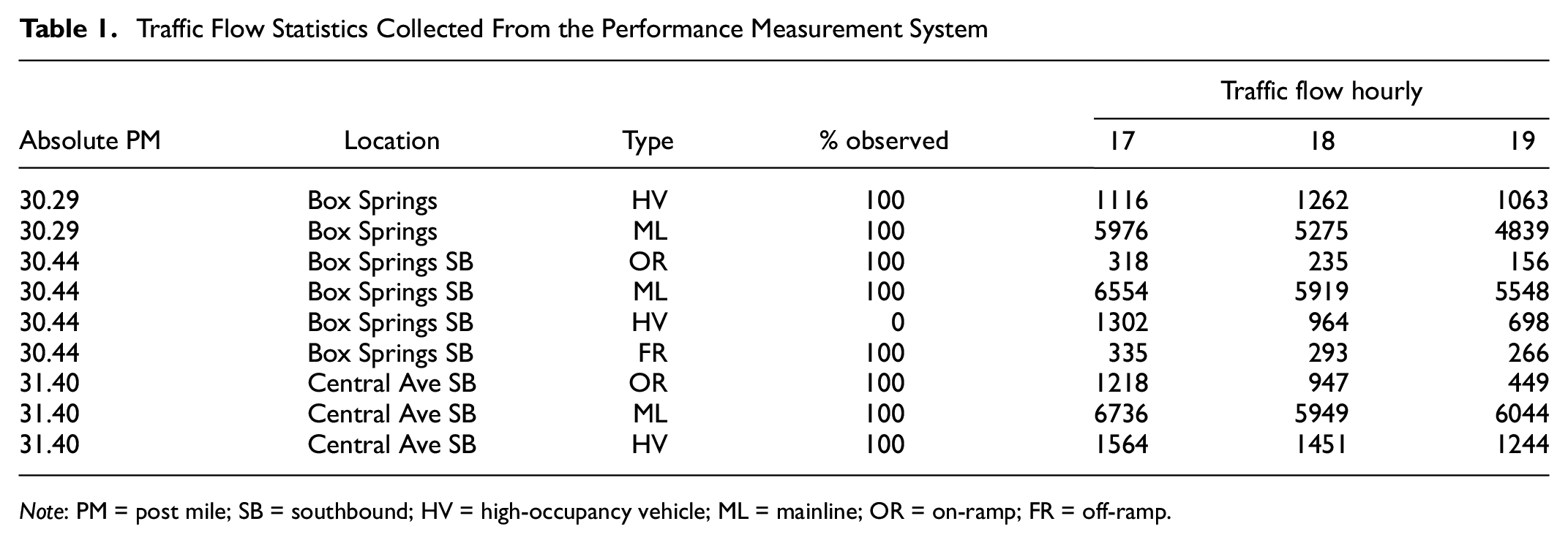
Note: PM = post mile; SB = southbound; HV = high-occupancy vehicle; ML = mainline; OR = on-ramp; FR = off-ramp.

q_{HV, Box Spring SB} = q_{HV + ML + OR, Central Ave SB} - q_{FR, + ML, Box Spring SB}

(1)

where q represents traffic flow, while FR, OR, ML, and HV represent the off-ramp, on-ramp, mainline, and HOV, respectively. The traffic flow at a finer resolution is calibrated using the ratio calculated from the hourly data. Figure 8 shows the traffic flow comparison before and after calibration. As we can see from Figure 8a, the traffic flow in the MF lane has an abrupt change at around PMs 32 and 32.9 and was fixed through the calibration process, with the result shown in Figure 8b. In Figure 8c, the original HOV traffic flow has a sudden change at around PMs 32 and 30.5, especially after 6 p.m., and we can see that the traffic flow no longer has those abrupt changes after calibration.

Figure 7.

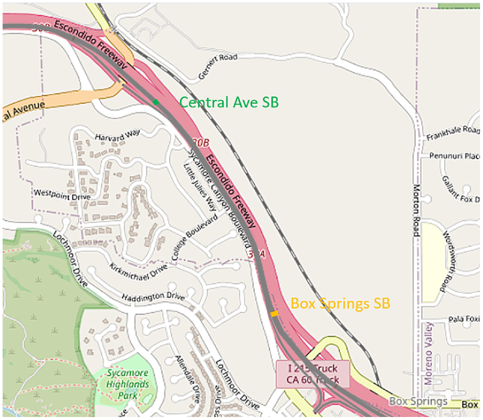
Location of the loop detectors on I-215 southbound (SB). The two detectors at Central Ave SB and Box Springs SB are labeled with green and yellow, respectively. (Color online only)

Figure 8.

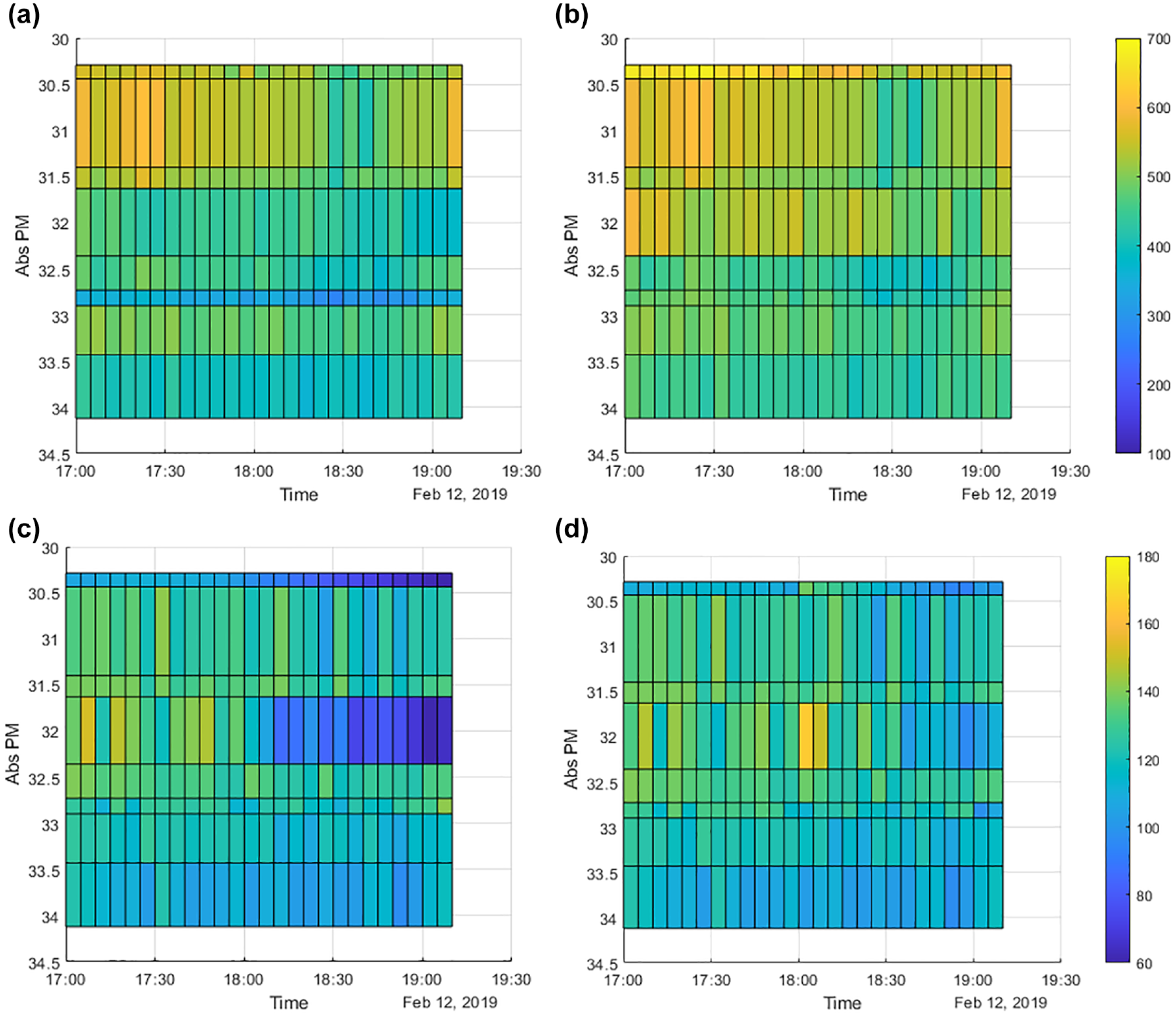
Comparison between original and calibrated traffic flow, absolute post mile (PM) versus time on I-215 southbound: (a) original mixed flow (MF) traffic flow, (b) calibrated MF traffic flow, (c) original high-occupancy vehicle (HOV) traffic flow, and (d) calibrated HOV traffic flow.

In the Vissim model, the link-level parameters, such as Link Behavior Type and Link Gradient, were calibrated based on the link data from the real world. The global parameters in Vissim, including the car following headway time and lane change safety reduction factor, were searched using a brute-force search algorithm over a selected range. As the best set of global parameters with the minimum hourly traffic flow difference between the simulation scenario and the ground truth, the final values of the headway time and safety reduction factor for the Merge link type were set to be 1.8 s and 0.4, respectively, and the same set of values for the Freeway link type were set to be 1.7 s and 0.6, respectively.

We then used the Caltrans guidelines ( 15 ) and followed the authors’ previous work ( 16 ) to validate our model quantitatively. The Geoffrey E. Havers (GEH) statistic and traffic flow error calculated using the data collected from each loop detector (nine MF detectors and nine HOV detectors southbound, eight MF detectors and eight HOV detectors northbound) are shown in Table 2. The GEH statistic is calculated using the following equation:

Table 2.

Summary of Validation Targets and Results

Criteria and measures	Acceptability targets	Validation results
Hourly flows: simulated versus observed
Individual link flows
Within 100 veh, for flow < 700 veh	>85% of all cases	100% of 0 cases
Within 15%, for 700 veh < flow < 2700 veh	>85% of all cases	88.2% of 17 cases
Within 400 veh, for flow > 2700 veh	>85% of all cases	88.2% of 17 cases
Total link flows-within 5%	All accepting links	0.203%
GEH statistics—individual link flow (GEH < 5)	>85% of all cases	88.2% of 34 cases
GEH statistics—total link flows (GEH < 4)	All accepting links	0.687
Visual audits
Individual link speeds
Visually acceptable speed–flow relationship	To analyst’s satisfaction	Satisfied
Bottlenecks
Visually acceptable queuing	To analyst’s satisfaction	Satisfied

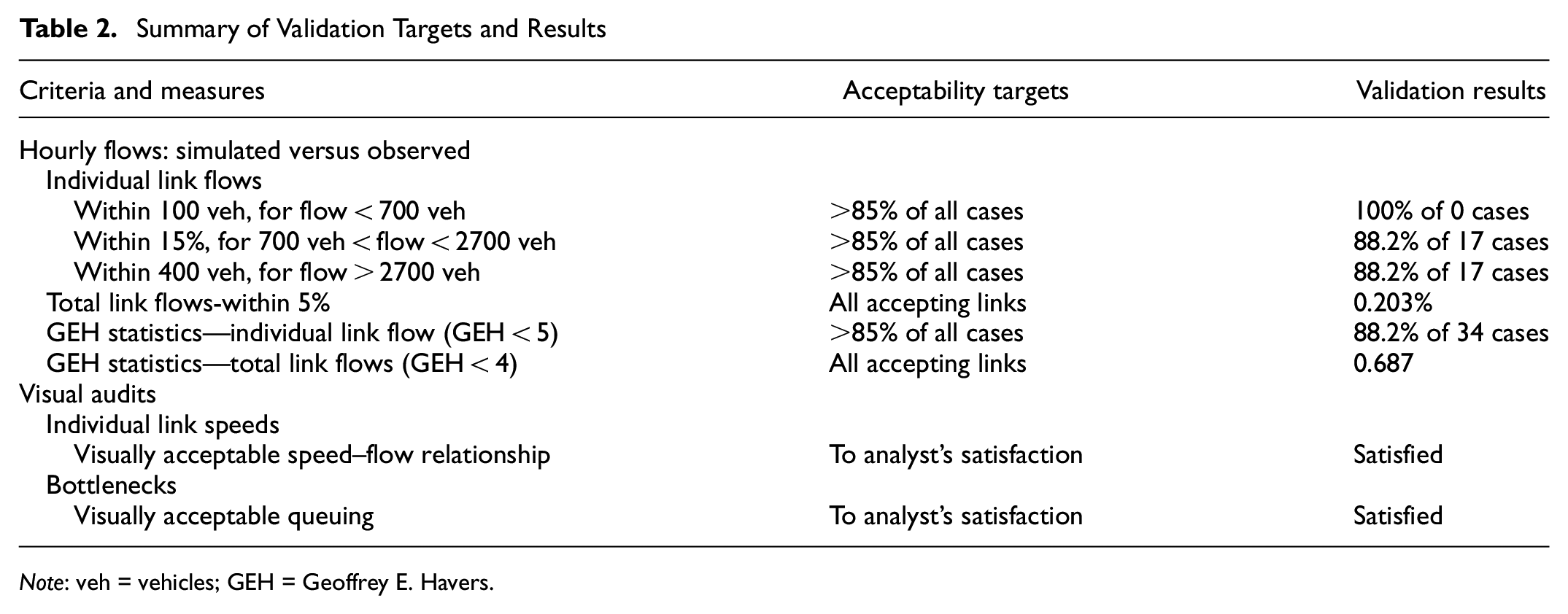
Note: veh = vehicles; GEH = Geoffrey E. Havers.

GEH = \sqrt{2 \times {(q_{s} - q_{o})}^{2} / (q_{s} + q_{o})}

(2)

where $q_{s}$ is the simulated flow and $q_{o}$ is the observed flow. As shown in the table, over 85% of all cases are in the acceptable range for each criterion, and the GEH statistic of total link flows is smaller than 5. The results verify that the simulated traffic network has been successfully calibrated according to real-world traffic.

After identifying the optimal set of parameters, we also tested other seed numbers and picked a total of five seeds that satisfied the criteria to increase the number of samples. As mentioned in the second section, we also coded two other simulation networks of the same freeway section—one with a new FC HOV lane and another one with a new PC HOV lane. We added the new HOV lane to the median of the freeway section and applied the verified parameters from the baseline simulation network to the new simulation networks. More details on simulation setup and numerical results are provided in the next section.

Results

We applied the full and PC HOV lane configurations to reduce traffic congestion and increase vehicle throughput in HOV lanes on the selected section of I-215. As shown in Figure 9, within the 5.1-mi study section of I-215 between PM 35 and PM 30, the lengths of the FC HOV lane (labeled in red) and the PC HOV lane (labeled in blue and green) are 4.6 and 3.5/1.1 mi, respectively. For the FC plan, the entire contraflow HOV lane between PM 35 and PM 30.8 will be used for northbound traffic in the morning, and be reversed for southbound in the afternoon and later. For the PC design, the added HOV lane segment between PM 35 and PM 31.8 will be utilized as the contraflow HOV lane to serve northbound traffic in the morning and southbound traffic in the afternoon or later. The added HOV lane segment between PM 31.8 and PM 30.8 will be designed for northbound only. As shown in the magnified views (a–c), for the PC plan, the switching point from the contraflow HOV lane to the northbound-only added HOV lane was selected to be the location that is usually free of congestion according to the typical traffic speed maps. In addition, the transition points between dual HOV lanes and single HOV lanes (e.g., locations a–c in Figure 9) were placed away from the bottleneck around on-ramp or off-ramp areas to avoid interfering with weaving traffic. Figure 10 shows schematic views of the existing design (top), PC (middle) and FC (bottom) with the labeled PM of each on-ramp, off-ramp, and dual HOV lane starting and ending locations. The two figures, Figures 9 and 10, help visualize the study site and the proposed solutions.

Figure 9.

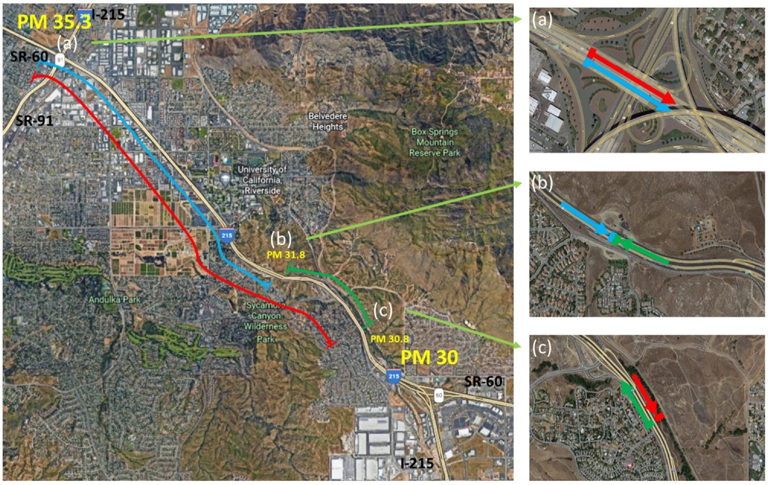
Map of start and end locations of partial contraflow and full contraflow high-occupancy vehicle lanes during afternoon peak hour with magnified views (a)–(c). (Color online only.)

Figure 10.

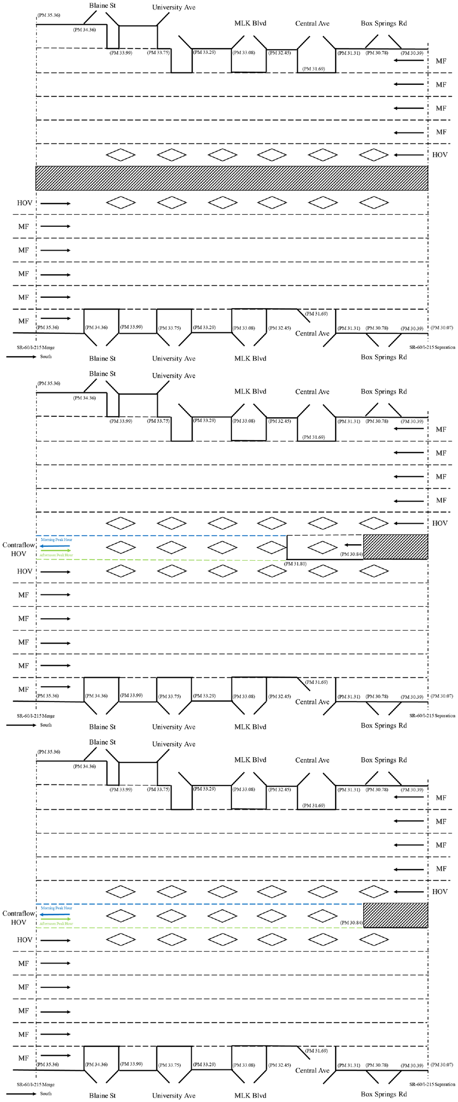
Schematics of the existing design (a), partial contraflow (b), and full contraflow (c) on I-215.

Five simulation runs with different seed numbers were made in each of the baseline, PC HOV, and FC HOV networks. The evaluation metrics, including the VMT, vehicle hours traveled (VHT), average travel speed (Q = VMT/VHT), and average vehicle delay were obtained and compared among the different networks, as shown in Figure 11 and summarized in Table 3. Vehicle delay is defined as the duration of the delay caused by the queues formed in the congestion.

Table 3.

Comparison of Performance Metrics Among Different High-Occupancy Vehicle Designs

Performance metrics	Southbound			Northbound		Combine
Performance metrics	Baseline	PC	FC	Baseline	PC	Baseline	PC	FC
VMT (mile)	39,566	39,796	39,895	31,938	31,650	71,504	71,446	71,833
VHT (hour)	1048	934	726	654	628	1702	1562	1380
Q = VMT/VHT (mph)	37.8	42.6	55.0	48.8	50.4	42.0	45.7	52.1
Delay (s)	134.6	98.3	32.8	59.7	51.7	101.0	77.4	45.0

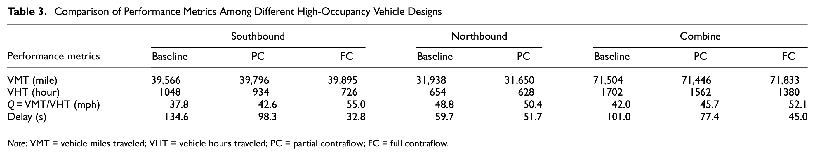
Note: VMT = vehicle miles traveled; VHT = vehicle hours traveled; PC = partial contraflow; FC = full contraflow.

Figure 11.

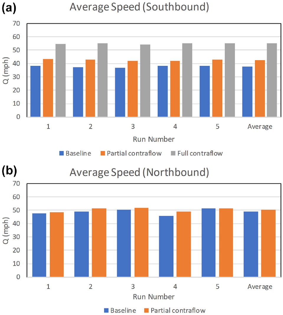
Average travel speed in southbound (a) and northbound (b) directions during the afternoon peak period.

According to Figure 11, the baseline network performs the worst with respect to average travel speed, reaching around 40 mph southbound and 50 mph northbound. In the southbound direction, the FC configuration has the highest average travel speed in all simulation runs, while the PC configuration performs better than the baseline but worse than the FC configuration. In the northbound direction, a similar increase in average travel speed can be observed when comparing the baseline and the PC networks. Note that the FC configuration does not apply to the northbound direction, since both directions cannot have an extra HOV lane at the same time and only the afternoon peak period is simulated. Therefore, the average speed of the northbound direction for the FC configuration will be the same as the baseline.

Table 3 provides the average values of the performance metrics from all five simulation runs. The values are provided separately for each travel direction of the freeway and combined. As can be seen from the table, in the southbound direction, the average travel speeds of the freeway with the additional FC HOV lane are 46% and 30% higher than that of the freeway with no additional HOV lane and the freeway with an additional PC HOV lane, respectively. The average delays of the freeway with an additional FC HOV lane are also reduced by 76% and 67%, respectively. In the northbound direction, the average travel speed of the freeway with additional PC HOV lane is 3% higher than that of the freeway with no additional HOV lane. The average delay of the freeway with an additional PC HOV lane is also reduced by 14% compared with the freeway with no additional HOV lane. When we combine the two directions and evaluate them together, the FC configuration outperforms the PC configuration with an increase in average speed of 14% and a decrease in delay of 42%. The possible explanation for the better average performance of the FC HOV lane southbound over the two PC HOV lanes in both directions is as follows:

for the northbound direction, as the baseline traffic is not very congested, the average speed and delay improvement from an additional HOV lane is not as significant as the other direction;

for the southbound direction, because of the highly congested traffic from the upstream freeways, the PC strategy will create a new bottleneck at the end of the additional HOV lane and cause additional delay when two HOV lanes merge to one.

To better visualize the effect of the additional HOV lane on traffic speeds, Figures 12 –14 show the HOV lane and MF lane speeds of all detectors in the baseline, PC HOV, and FC HOV networks, respectively. As can be seen from Figure 12, the traffic speed starts to drop significantly starting from 5:10 p.m. at PM 32, and most of the traffic speeds in the baseline drop below 30 mph in both the HOV and MF lanes of the study section between PMs 31.5 and 34.0. The MF lane also appears to be more congested than the HOV lane, with a lower average speed. On the other hand, there is little congestion in the FC HOV network shown in Figure 14, while the PC HOV network has some severe congestion at around PM 32.0 where the dual HOV lanes end. In general, the additional HOV lane reduces traffic congestion on the study freeway section, not only in the HOV lanes but also in the MF lanes. The congestion reduction in the HOV lanes can help alleviate or even eliminate the issue of performance degradation in these HOV facilities. For instance, the FC HOV configuration increases the average travel speed in the southbound HOV facility from 37.8 to 55.0 mph, which is enough to lift this HOV facility out of the degradation status.

Figure 12.

Traffic speed southbound for (a) the high-occupancy vehicle lane and (b) mixed flow lanes in the baseline. The direction of the traffic flow is from absolute post miles (PMs) 34 to 30.

Figure 13.

Traffic speed southbound for (a) the partial contraflow (PC) high-occupancy vehicle lane and (b) PC mixed flow lanes.

Figure 14.

Traffic speed southbound for (a) the full contraflow (FC) high-occupancy vehicle lane and (b) FC mixed flow lanes.

Conclusion

In this study, we evaluated and compared two contraflow HOV lane designs for reducing traffic congestion and mitigating HOV lane performance degradation using traffic microsimulation networks calibrated based on real-world traffic data. We selected the afternoon peak hour as the simulation period and studied the impact of adding a contraflow HOV lane on traffic performance in both directions of the freeway. The simulation results showed that the FC design outperforms the PC design with respect to having 14% higher average speed and 42% less delay. Compared with the baseline, the FC design would increase the average speed by 24% and decrease the delay by 55%. Most importantly, the FC design would increase the average speed in the southbound HOV lane from 37.8 to 55.0 mph, which is enough to lift this HOV facility out of degradation status.

The research conclusion above is based on the simulation results of a specific freeway section with certain traffic patterns during the afternoon peak hour. The benefits of implementing a contraflow HOV lane to supplement the existing HOV lanes, as well as the pros and cons of the different designs, may vary for each freeway and HOV facility. For future work, additional simulation scenarios can be created to evaluate the benefits of the two contraflow HOV lane designs during morning peak hours. Safety performance of the different contraflow HOV lane designs can also be studied. In addition, a method for choosing the most appropriate starting and ending locations of a contraflow HOV lane should be developed in the future.

Footnotes

Acknowledgements

The research team acknowledges the program support from Joe Rouse, Don Howe, Jose Perez, Melissa Clark, Jose Camacho, and Gurprit Hansra during the course of the project. We also thank Caltrans District staff and other stakeholders for comments and feedback on the research.

Author Contributions

The authors confirm contribution to the paper as follows: study conception and design: K. Boriboonsomsin, P. Hao; data collection: Z. Wei; analysis and interpretation of results: Z. Wei, P. Hao, K. Boriboonsomsin, M. Barth; draft manuscript preparation: Z. Wei, P. Hao, K. Boriboonsomsin. All authors reviewed the results and approved the final version of the manuscript.

Declaration of Conflicting Interests

The author(s) declared no potential conflicts of interest with respect to the research, authorship, and/or publication of this article.

Funding

The author(s) disclosed receipt of the following financial support for the research, authorship, and/or publication of this article: This research was conducted in fulfillment of Agreement No. 65A0724, Task 2353 “Alternative HOV Lane Operational Strategies for Congestion Mitigation in California,” under the sponsorship of the California Department of Transportation (Caltrans).

ORCID iDs

Zhensong Wei

Peng Hao

Matthew Barth

Kanok Boriboonsomsin

The views expressed are those of the authors and do not necessarily represent those of Caltrans or the State of California.

References

California Department of Transportation. 2019 California High-Occupancy Vehicle Facilities Degradation Report and Action Plan. California Department of Transportation, Sacramento, December 2020. https://dot.ca.gov/-/media/dot-media/programs/traffic-operations/documents/managed-lanes/hov/2019-california-hov-facilities-degradation-report-action-plan.pdf.

Skowronek

D. A.

Ranft

S. E.

Cothron

A. S.

Evaluating HOV Lanes in the Dallas Area. Project Summary Report 7-4961-S. Texas Transportation Institute, Texas A & M University, June 2004.

Zhao

James

R. M.

Xiao

Bared

A Capacity Estimation Model for a Contraflow Left-Turn Pocket Lane at Signalized Intersections. Transportation Research Record: Journal of the Transportation Research Board, 2018. 2672: 22–34.

Wolshon

Lambert

Reversible Lane Systems: Synthesis of Practice. Journal of Transportation Engineering, Vol. 132, No. 12, 2006, pp. 933–944.

Waleczek

Geistefeldt

Cindric-Middendorf

Riegelhuth

Traffic Flow at a Freeway Work Zone With Reversible Median Lane. Transportation Research Procedia, Vol. 15, 2016, pp. 257–266.

Zhao

Liu

Yang

Integrated Design and Operation of Urban Arterials With Reversible Lanes. Transportmetrica B: Transport Dynamics, Vol. 2, No. 2, 2014, pp. 130–150.

Zhou

Mao

Dai

Liu

Bao

Collaborative Control Optimization on Reversible Lanes in Intersection Group Under Intelligent Vehicle Infrastructure Cooperative System. Journal of Advanced Transportation, Vol. 2020, 2020, pp. 1–12.

Mao

Zhou

Zhang

Dai

Design of Real-Time Dynamic Reversible Lane in Intelligent Cooperative Vehicle Infrastructure System. Journal of Advanced Transportation, Vol. 2020, 2020, pp. 1–8.

Meng

Khoo

H. L.

Optimizing Contraflow Scheduling Problem: Model and Algorithm. Journal of Intelligent Transportation Systems, Vol. 12, No. 3, 2008, pp. 126–138.

10.

Pérez-Méndez

Gershenson

Lárraga

M. E.

Mateos

J. L.

Modeling Adaptive Reversible Lanes: A Cellular Automata Approach. PloS One, Vol. 16, No. 1, 2021, p. e0244326.

11.

PTV Group. Traffic Simulation Software. Traffic Simulation Software | PTV Vissim | PTV Group. https://www.ptvgroup.com/en/solutions/products/ptv-vissim/. Accessed December 10, 2021.

12.

California Department of Transportation. Caltrans Pems. Caltrans. https://pems.dot.ca.gov/. Accessed December 10, 2021.

13.

OpenStreetMap Contributors. Planet Dump [Data File From $date of Database Dump$]. 2015. https://planet.openstreetmap.org.

14.

Google Maps. “I-215 Freeway Segment.” Typical Traffic Satellite Image. 2021. https://www.google.com/maps/@33.9689054,-117.3295729,14z/data=!5m1!1e1?hl=en&authuser=0. Accessed March 9, 2021.

15.

Dowling

Skabardonis

Alexiadis

Traffic Analysis Toolbox, Volume III: Guidelines for Applying Traffic Microsimulation Modeling Software. United States. Federal Highway Administration. Office of Operations, Washington, D.C., June1, 2004.

16.

Shan

Hao

Boriboonsomsin

Barth

Chen

Partially Limited Access Control Design for Special-Use Freeway Lanes. Transportation Research Part A: Policy and Practice, Vol. 118, 2018, pp. 25–37.

Evaluating Contraflow High-Occupancy Vehicle Lane Designs for Mitigating High-Occupancy Vehicle Lane Performance Degradation