Sage Journals: Discover world-class research

Abstract

Mode choice modeling is imperative for predicting and understanding travel behavior. For this purpose, machine learning (ML) models have increasingly been applied to stated preference and traditional self-recorded revealed preference data with promising results, particularly for extreme gradient boosting (XGBoost) and random forest (RF) models. Because of the rise in the use of tracking-based smartphone applications for recording travel behavior, we address the important and unprecedented task of testing these ML models for mode choice modeling on such data. Furthermore, as ML approaches are still criticized for leading to results that are hard to understand, we consider it essential to provide an in-depth interpretability analysis of the best-performing model. Our results show that the XGBoost and RF models far outperform a conventional multinomial logit model, both overall and for each mode. The interpretability analysis using the Shapley additive explanations approach reveals that the XGBoost model can be explained well at the overall and mode level. In addition, we demonstrate how to analyze individual predictions. Lastly, a sensitivity analysis gives insight into the relative importance of different data sources, sample size, and user involvement. We conclude that the XGBoost model performs best, while also being explainable. Insights generated by such models can be used, for instance, to predict mode choice decisions for arbitrary origin–destination pairs to see which impacts infrastructural changes would have on the mode share.

Keywords

mode choice interpretable machine learning revealed preference smartphone tracking sensitivity analysis travel behavior

In the field of transportation, mode choice behavior has been researched for many years ( 1 , 2 ). There are two main objectives in developing models that reflect this behavior. They can be used to predict the anticipated individual choices and mode share, and they help one to explain and understand the factors influencing such behavior. In recent years, this field has seen many contributions that use machine learning (ML) approaches ( 3 – 6 ) instead of conventional discrete choice models (DCMs). While ML approaches typically perform well at predicting mode choice behavior, they have long been referred to as a “black box.” Their immense complexity (compared to DCMs) makes it difficult to infer, back-track, and explain individual predictions. Nonetheless, these approaches have increasingly become explainable and interpretable.

Aside from new modeling approaches for mode choice behavior, we see a gradual rise of a new form of travel data: (semi-)passive travel diaries, that is, automated tracking-based revealed preference (TRP) data ( 7 ). Typically, participants’ behavior is recorded in a smartphone app and travel diaries are automatically generated. Previously, the following two survey types were the norm. In stated preference (SP) surveys, participants report their typical behavior or respond to hypothetical scenarios. In self-reported conventional revealed preference (CRP) travel diaries, each trip is noted down in a travel diary. Both survey types are known to face issues such as an underreporting of trips, user manipulation, bias, or error (e.g., wrong starting time) ( 8 , 9 ), and are inferior in quality, resolution, and granularity compared to tracking-based travel diaries. TRP data has exact and generally reliable start and end times of trips, as well as precise start and end locations. These aspects enable the precise consideration of a wide range of potential additional influencing factors for mode choice, such as infrastructure-related features, accurate weather data, or information about unchosen modes. A downside of TRP data is the inability to explicitly ask users about their mode choice behavior or perceived stress. However, the ability to generate and obtain a high number of high-quality features renders ML a promising modeling approach for this type of data.

In the context of ML for mode choice modeling, promising results have been achieved for SP and CRP data ( 10 – 12 ). Thus far, while these have been found to be viable and accurate, only a few studies have considered the explainability of the ML models. In this paper, we will address two aspects that are yet to be explored. Firstly, we apply an extreme gradient boosting (XGBoost) model (often the best performing among SP/CRP studies) to the emerging TRP data to predict mode choice behavior. Secondly, we conduct an in-depth analysis of the explainability of such an approach. As shown in Figure 1, these are applied to unique long-duration semi-passive tracking-based travel diary data. The Mobilität.Leben study comprises data from May 2022 to June 2023 and a heterogeneous user base, most of which travel in the Greater Munich area of around 6000 km².

Figure 1.

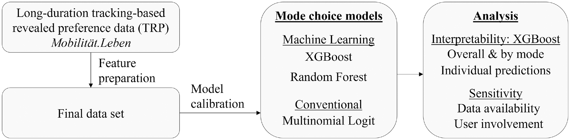
Overview of the structure of the paper.

The outline of this paper is as follows. Firstly, the current literature is reviewed and the research gap is identified, on which the case study data is introduced. In the methodology, three models are selected and described, and the data preparation and model calibration are detailed. Next, the results are presented both at the overall and mode-specific level. The best-performing model is analyzed in detail concerning its explainability, and the most important features contributing to each mode of transport are discussed in depth. Lastly, a sensitivity analysis sheds light on how data availability and quality constraints can affect model performance.

Background and Literature Review

When dealing with TRP data, it is important to note that there are fully passive and semi-passive travel diaries. For semi-passive travel diaries, the user has the option to validate and correct the draft travel diaries that are generated by the smartphone application. The benefit of this is that in addition to having data that is precise in space and time, given a reliable and committed user, it is also accurate with respect to travel behavior, mode, and purpose detection. Therefore, both types of data are equally suitable for ML models, yet user involvement increases the data quality. We anticipate that TRP data will become increasingly common in travel survey design.

Conventional approaches in the field of mode choice modeling, in brief, include multinomial logit regression (MNL), nested, and mixed logit models. These have frequently been used as benchmarks for novel ML approaches. The ML approaches for SP data have consistently achieved higher accuracy when compared to conventional models ( 13 ). For instance, Zhao et al. ( 10 ) observed more than 20% and García-García et al. ( 4 ) more than 15% difference between the best ML classifier (XGBoost) and MNL or mixed logit. Wang et al. ( 14 ) made an extensive comparative review including 86 ML classifiers. Among these studies, the XGBoost and random forest (RF) approaches consistently performed best (if either was considered) with few exceptions. They outperform DCMs, including MNL, naive Bayes, linear regression, and so forth, and other ML approaches, such as support vector machines and artificial and convolutional neural networks. The reader is referred to Wang et al. ( 14 ) for an extensive overview. It will later be observed that the price of public transport (PT) is an important factor in our case study, yet it is often not considered in these ML models. With regards to revealed preference (RP) data, there is literature about CRP data ( 4 , 11 , 12 , 15 , 16 ). However, for TRP data very few studies have been made. To the best of the authors’ knowledge, only Buijs et al. ( 17 ) has performed mode choice modeling on TRP data using a ML approach (artificial neural network); however, the interpretability of the results is not investigated.

Overall, the area of mode choice modeling in transportation has increasingly observed that ML approaches may be explainable, to an extent. Pineda-Jaramillo and Arbeláez-Arenas ( 11 ) and Tamim Khashifi et al. ( 13 ) used so-called SHapley Additive exPlanations (SHAP) values and explored their interaction effects. The SHAP values essentially measure the relative contribution of each variable to the model output. Zhao et al. ( 10 ) and Richards and Zill ( 15 ) assessed feature importances and partial dependencies. The study of explainability is of great importance when using ML models for mode choice modeling to avoid implausible mode choice behavior. If one cannot explain a mode prediction for a given trip, then one cannot interpret the reasons for such behavior; however, this is crucial for transportation planners, for example, to improve infrastructure.

Based on the identified gap of ML models for TRP data, this paper will apply two such models (and a DCM benchmark model) to TRP data. Only three models are selected, in contrast to Wang et al. ( 14 ), to leave room for discussion and extended analysis. We consider it imperative to assess the explainability of the results in depth; this involves an analysis of the individual modes, which has thus far only been done by Bhuiya et al. ( 18 ) for data recorded in Bangladesh. Furthermore, a sensitivity analysis will give insight into the impact of limited data and feature availability.

Case Study Area and Data

Case Study Area

The study area for this research is the city of Munich, located in southern Germany, and its surrounding area. Munich is the third largest city in Germany and has the highest population density. A well-developed road network spreads out from the city center. The transportation system in the city includes major arterial roads, residential streets, a comprehensive PT system, and a developed pedestrian and bicycle network. Figure 2 provides a visual representation of the city’s layout and the trajectory data used here, where the darker shades of blue correspond to a higher density of recorded trips. The area considered for this study includes the entire operating area of Greater Munich’s PT service provider (MVV), which comprises the subway, bus, S-Bahn, and tram network.

Figure 2.

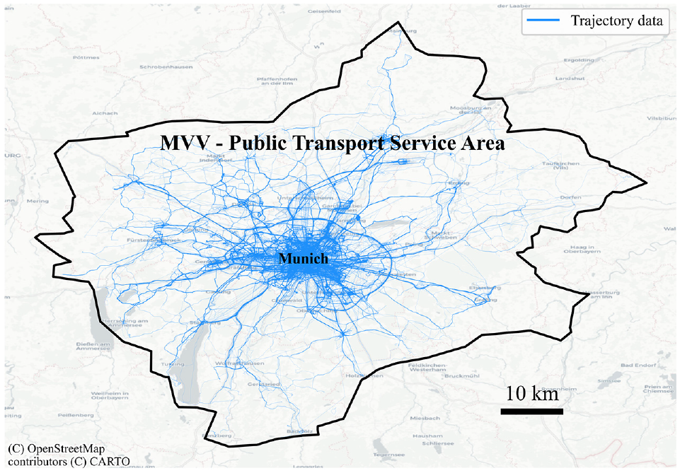
Study area: the public transport service area encompassing Greater Munich (Germany) is outlined in black. The Global Positioning System data’s geographical distribution is visualized in varying shades of blue, indicating the density of recorded trajectories.

Dataset

The selected models were applied to data from a unique long-duration TRP study: Mobilität.Leben ( 19 ), which translates to “mobility.life.” To study the impact of the three-month 9-Euro ticket in Germany (and later on its successor, the Deutschlandticket) on travel behavior, a series of survey waves with 2569 participants was conducted. The surveys inquired about mobility behavior and sociodemographic data, which are in part used here. Of these survey participants, 1192 additionally installed a smartphone application, which automatically generated draft travel diaries based on trajectories recorded by their smartphone. The app users were able to accept (validate) and, if necessary, correct these draft travel diaries.

The travel diaries were processed to reduce noise and low-quality recordings stemming from unreliable users or erroneous Global Positioning System (GPS) tracking. In brief, the data was cleansed (e.g., removing abnormally short tracks/stays or speed outliers), processed (merging of sequential tracks/stays of the same mode/purpose, trip detection), and enriched (incorporating other data sources, such as weather, alternative travel times, sociodemographic data), as detailed by Dahmen et al. ( 20 ). The entire study lasted from June 2022 to July 2023, where, on average, users participated in the mobility tracking for 209 days. This led to a total of 882,790 trips.

Methodology

In this section, we outline the selection of the mode choice models, two of which are ML-based and one of which is a conventional DCM method. In addition, the data preparation and model calibration are described.

Model Selection

The model selection for this study was based on the literature review, which revealed the XGBoost and RF models to be both common and the best-performing algorithms for SP and CRP data. Therefore, these models were selected to be applied to TRP data in this study. These two models are compared to a common DCM, the MNL.

XGBoost

An XGBoost model is an advanced form of decision trees, first proposed by Friedman ( 21 ). Conceptually, one can think of a decision tree as a model that learns patterns (in our case mode choice behavior) within data and makes a final decision on the data (such as the chosen mode), which comprises many individual decisions (What is the temperature? Or income?). XGBoost models adopt an incremental training approach, gradually learning (training) one tree at a time, starting with smaller low-complexity trees that have low learning capacity (weak learners). Trees are pruned to prevent overfitting, that is, learning patterns too well, therefore reducing transferability to new data. The model aims to consistently learn from the mistakes of previous trees (at a specific learning rate). The gradual performance improvement up to the final tree is measured using a loss function, which quantifies the error rate between predictions and true values. The gradient of this loss function is key to the learning process in this type of gradient boosting model and is subject to optimization to ensure fast, efficient learning. Such a combination of different model instances is known as an ensemble. The reader is referred to Joshi ( 22 ) for an in-depth explanation. The learning rate, loss function, regularization (to avoid overfitting), maximum allowed depth of individual trees (i.e., the number of sub-decisions), and overall number of trees (iterations) all have to be carefully set to ensure optimal learning with respect to accuracy and runtime.

RF

RF models are also based on decision trees, yet they build these independently in parallel, rather than sequentially. Furthermore, these trees are trained on random subsets of the data and features and are later aggregated, aiming to create an accurate yet robust model. Apart from the maximum number of trees and tree depth, the RF’s hyperparameters also include the maximum number of samples that may be used to train each tree ( 18 , 22 ).

MNL

MNL has a lower degree of complexity. It is a statistical method, based on utility theory, that is an extension of logistic regression, which is binary by nature (not multi-class). It aims to approximate the mutually exclusive transportation modes, commonly using logistic regression and maximum likelihood estimation ( 16 , 23 ). Hyperparameters include a C-value, which can be used for regularization, and selecting a solver, which is the algorithm used to optimize the model’s coefficients (weights).

Comparison

Overall, the MNL stands out because of its explainability, making it the easiest model to interpret. However, the interpretations cannot necessarily be made with confidence, as the model assumes linearity in parameters. The parameters themselves can be non-linear though. The low complexity reduces the likelihood of overfitting. In comparison, RF models can be highly complex. They can learn more advanced non-linear patterns and are also robust to overfitting. On the downside, they are less suitable for imbalanced training data. XGBoost models share the high learning capacity of RF algorithms, but they can be computationally expensive. They are known for their good prediction accuracy. In addition, an advantage of XGBoost is that it can handle missing values (e.g., if an attribute of a user is unknown). In contrast, for the MNL and RF approaches, missing values must be imputed to use them as training data.

Data Preparation

In this paper, only a subset of the Mobilität.Leben data is used to ensure high-quality data. We use data from September 2022 to March 2023 to exclude special PT fare policies: the 9-Euro ticket and the Deutschlandticket. Only trips (partially) within Greater Munich’s PT service area are considered to limit the study’s spatial coverage and facilitate PT cost and travel time estimation. Furthermore, we exclude round trips, which start and end in the same place (typically leisure walks), as these do not reflect travel behavior with a different origin and destination. To ensure accurate travel data, we selected trips from reliable and involved users, which we defined as users that were actively correcting, that is, editing the draft travel diaries near the time of recording. With respect to the transport mode, for multimodal trips the main mode is the mode with the largest travel distance. The modes of transportation were grouped into four categories: walk, car, bike, PT. The modes airplane, boat, and other were excluded. As the mode share of walking (37.7%) drastically differed to car (20.6%), bike (20.0%), and PT (21.7%), the number of walking trips was reduced to match the other modes to lessen the imbalance in the data. In total around 60,000 trips were used.

Feature Preparation

A wide range of features (i.e., variables) was selected, based on the literature and the available and derivable values. These features comprise trip information, sociodemographic data, weather ( 24 ), estimated travel times and cost by mode, and infrastructure ( 25 ). Table 1 shows the individual features of each feature group and the respective data sources. All data was normalized before training the models, that is, scaled to zero-mean and unit variance. With respect to car ownership, such information is known for 81% of the trips. The remaining trips are assigned the label “unknown.” The estimated travel times were obtained using the TomTom API (car) ( 26 ), which considers historic traffic patterns, and the open-source tool OpenTripPanner (walk, PT, bike) ( 27 ). In all cases the estimated rather than the actual travel time was used, as the latter could reveal information about the chosen mode. In some cases, no travel times were computed for PT or car trips, for example, for very short routes or because of the lack of PT service. These missing values were imputed in a way that would convey the unattractiveness of choosing that mode (as it is not available): because of the collinearity of the PT and car travel time with the time by walking, a 95th percentile regression (a form of quantile regression) is fitted to these (PT/car time versus walk time) and used for the imputation. The estimated cost of traveling by car is calculated based on the distance of the car route. The PT cost is based on the price of an appropriate single ticket given the local zone-based PT pricing structure. The PT cost also considers whether a person is subscribed to a monthly PT ticket, in which case the price per trip is set to the monthly price divided by the number of trips. For the monthly price, we assume €64, which is the price of a monthly ticket within one of the local transport zones. The cost of walking and cycling was set to zero as no relevant monetary costs arise for these.

Table 1.

Input Features Used for Modeling (Category Level Used in Example in Bold)

Feature	Source	Example	Notes/category encoding: [0, …, n]
Socio-demographic
Age	Survey	32 years	na
Income	Survey	0	[<1.5, 1.5–2.5, 2.5–4, >4] in k€
Employment status	Survey	1	[employee, student, both, neither]
Gender	Survey	2	[female, diverse, male]
Car ownership	Survey	0	[no, unknown (19% of trips), yes]
Weather
Precipitation	DWD ( 24 )	2 mm	Hourly, at city center
Temperature	DWD ( 24 )	16°C	Hourly, at city center
Relative humidity	DWD ( 24 )	82%	Hourly, at city center
Wind speed	DWD ( 24 )	1.5 m/s	Hourly, at city center
Estimated travel time & cost
Time by car	TomTom ( 26 )	17 min	na
Time by walking^a	OTP ( 27 )	72 min	na
Time by bike^a	OTP ( 27 )	27 min	na
Time by PT	OTP ( 27 )	34 min	na
PT transfers	OTP ( 27 )	1	na
PT cost	Derived	€5.6	Considers monthly PT pass
Car cost^a	Derived	€11.3	na
Trip information
Length	-	8700 m	Straight-line distance
Trip start time	-	15.0	Rounded to nearest full hour
Day of week	-	6	[Mon, Tue, Wed, Thu, Fri, Sat, Sun]
Infrastructure
Bike racks	OSM ( 25 )	2	No. within 200 m
PT stop density	OSM ( 25 )	1	No. within 800 m
Bike infrastructure quality	OSM ( 25 )	0.24	Ratio of length of roads with cycling infrastructure to those without

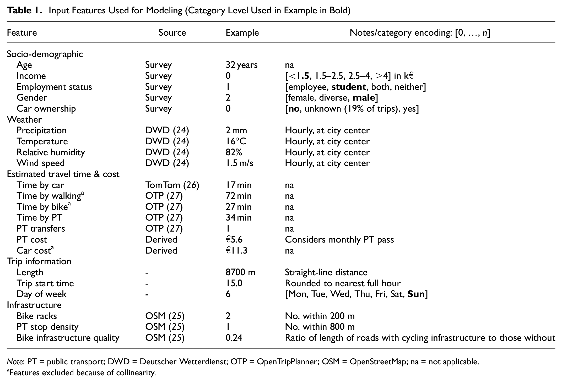
Note: PT = public transport; DWD = Deutscher Wetterdienst; OTP = OpenTripPlanner; OSM = OpenStreetMap; na = not applicable.

Features excluded because of collinearity.

A collinearity analysis was performed on the 22 features, as collinearities tend to lower the MNL’s performance and make it harder to explain the results. The standard Pearson correlation coefficients (a measure of the linear correlation between two variables [ 28 ]) were evaluated. Length, car cost, time by bike, and time by walking are highly correlated with each other (>0.96). Consequently, all but one of these (length) were removed, as they convey the same information sufficiently well. Time by car and time by PT also correlate with length, yet not enough to remove them. Furthermore, the statistical analysis of all features is shown in Table 2. It is noted that the high maximum PT price results from an individual having a PT pass but not using it sufficiently. If one has a monthly PT pass but only makes one PT trip in a month, the effective price of the trip will be the price of the PT pass. Furthermore, the number of bike racks is rarely over 40; this is only the case for two central train stations and two new development areas, where there is a bike rack in front of each building. The very high PT stop density values are also only found at one of the main train stations.

Table 2.

Statistical Distribution of Features

Categorical feature	Percentage share of each category (%)
Income	€1499 or less: 10, €1500–€2499: 14, €2500–€3999: 26, €4000 or more: 50
Employment status	Employee: 68, Student: 10, Both: 8, Neither: 14
Gender	Female: 50, Diverse: 1, Male: 50
Car ownership	No: 33, Unknown: 1, Yes: 66
Day of the week	Mon.: 15, Tue.: 16, Wed.:16, Thu.: 17, Fri.: 16, Sat.: 14, Sun.: 8
Numerical feature	Mean	SD	Min.	Max.
Age (years)	43.0	14.5	15.0	82.0
PT price (€)	1.8	2.2	0.1	63.2
Car price (€)	3.7	4.7	0.1	46.4
Time by PT (min)	34.9	30.7	1.0	981.0
Time by car (min)	12.6	9.5	0.4	74.8
PT transfers (no.)	0.5	0.8	0.0	5.0
Time by walking (min)	40.4	48.1	0.0	239.0
Time by bike (min)	20.1	29.4	0.0	240.0
Bike racks (no.)	3.1	5.5	0	80
PT stop density (no.)	12.5	11.2	0	125
Bike infrastructure quality	0.2	0.1	0.0	0.9
Precipitation (mm)	0.1	0.4	0.0	8.2
Temperature (°C)	11.3	7.1	-10.0	27.5
Relative humidity (%)	74.2	15.5	32.0	99.0
Wind speed (m/s)	2.4	1.2	0.3	8.9
Length (m)	3836.4	6070.8	0.0	68,449.3
Time of day (hour)	12.5	4.2	0	23

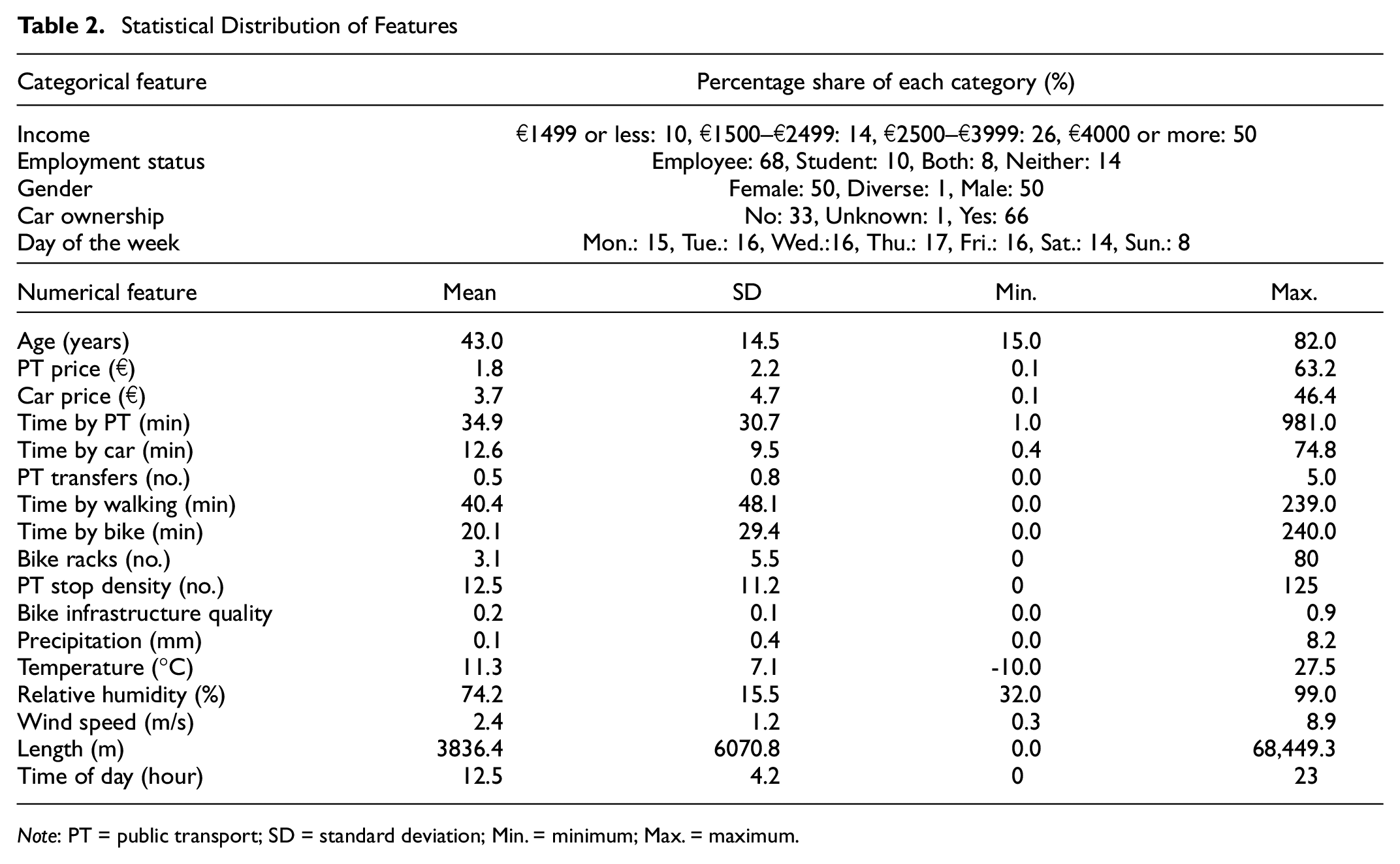
Note: PT = public transport; SD = standard deviation; Min. = minimum; Max. = maximum.

Model Calibration

Using the prepared dataset, the models’ hyperparameters were tuned using a grid-based approach (testing all combinations of a preselected set of parameter values) to determine the set that led to each model’s best mean training accuracy. The models were trained with 70% and tested with 30% of the data, and 10-fold cross-validation (CV) was employed to counteract overfitting and selection bias. CV means that the data is reshuffled before each of the 10 train–test runs.

The models were built in Python using XGBoost’s XGBClassifier and sklearn’s RandomForestClassifier and LogisticRegression. The final hyperparameters of the XGBoost model include a learning rate of 0.1 and 300 trees. The multi:softmax objective function is selected as we are dealing with a multi-class classification. The maximum tree depth is relatively high (maximum 30). A minimum child weight of 9 helps to avoid overfitting and reduces the model complexity. This also applies to the regularization measures (gamma: 0.01, lambda: 5). For the RF model, 250 trees and a maximum possible depth of 60 led to the best results. An “lbfgs” solver (limited-memory Broyden–Fletcher–Goldfarb–Shanno, capable of handling multi-class problems) was used to solve the MNL model with L2 loss (sum of all squared differences). The C-value was set to 2.5, that is, a relatively low penalty is applied to the coefficients during training.

The performance was measured based on accuracy, as this is commonly used in the literature ( 5 , 10 , 14 , 15 , 29 ). The accuracy of this multilabel classification problem was determined as follows, where $n$ is the number of samples and “ $1 ()$ ” is the indicator function: $(1 / n) \times \sum_{i = 0}^{n - 1} 1 ({\hat{y}}_{i} = y_{i})$ ( 30 ). As here the mode classes are split almost evenly, little bias is expected in the accuracy, therefore by definition the accuracy is expected to be similar to the recall ( 13 ). The standard deviation of the CV is also considered to assess the consistency of the results. The runtime will not be assessed, as even the longest training time was below 10 min for the final hyperparameters.

Results and Discussion

This section is split into three: firstly, the results of the three classification models will be compared overall and by mode. Next, the explainability of the best-performing model will be assessed in depth, ranging from the contribution of each feature to assessing individual predictions. Lastly, a sensitivity analysis will provide valuable insights about the model performance when subject to various data constraints.

Overall Results

Among the XGBoost, the RF, and the MNL models, the XGBoost model performed best when considering the mean accuracy: 79.0%. The RF was slightly inferior (76.3%) and the MNL performed poorly in comparison (57.7%), as shown in Table 3. This ranking of the three models is consistent with other studies, where XGBoost is either equally good or only slightly better than the RF ( 10 , 11 , 13 , 15 ). The XGBoost model also outperformed the RF and MNL in the standard deviation of the CV, at 0.28%, 0.78% and 0.44%, respectively; this implies that there is lower variation among the CV runs. The accuracies of such models can hardly be compared across studies, if there were any for TRP data, as the results are heavily affected by factors such as the data quality, size, and region.

Table 3.

Mean Accuracy of the Baseline Models (Overall and Mode-Specific Accuracy) and Model Variations (Overall Accuracy Only)

Description	Accuracy (%)
Description	XGBoost	RF	MNL
Baseline
Overall accuracy	79.0	76.3	57.7
Accuracy of PT predictions	79.3	77.3	66.5
Accuracy of bike predictions	76.3	77.7	62.2
Accuracy of car predictions	77.8	72.5	46.1
Accuracy of walk predictions	82.7	77.0	52.0
Variations in input features
No survey-based data (sociodemographic, PT monthly pass and car ownership)	76.0	73.2	56.8
No infrastructure data	77.4	75.0	54.9
No weather data	78.4	77.1	57.5
No alternative travel time data	78.5	76.8	53.3
Only trip data (length, time of day, weekday)	53.5	48.0	46.7
Including all collinear features	79.0	73.7	53.8
Variations in dataset size
10,000 trips per mode	77.6	74.5	56.9
3000 trips per mode	72.3	69.3	52.0
700 trips per mode	66.9	63.3	54.5
Variation in user involvement
Fully passive tracking (non-correcting users)	76.4	72.9	53.6

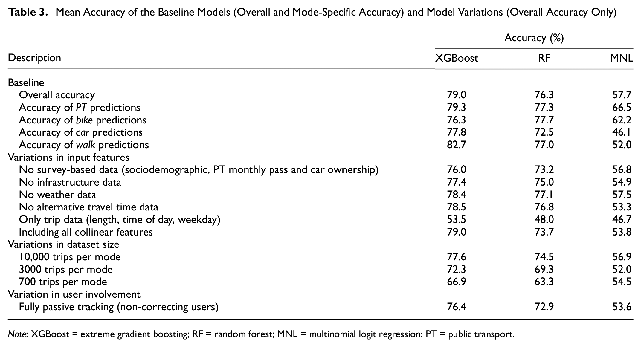
Note: XGBoost = extreme gradient boosting; RF = random forest; MNL = multinomial logit regression; PT = public transport.

When looking at the individual output classes (the four modes), the XGBoost model again surpassed the other models with respect to the average score, and for PT, car, and walk. For both the RF and the XGBoost, there was little deviation in the accuracy scores across the individual modes. The ML models are able to capture the patterns in the data well for all modes, which can, in part, be attributed to the low imbalance in the data. In the case of the MNL model, the model was better at predicting PT and bike trips than car and walk trips.

The confusion matrix for MNL (Figure 3a) reveals that walk trips were frequently classified as bike trips (36% of all walk trips); these matrices display the values of single runs. Falsely predicted car trips (45%) were often predicted as bike (28%) or PT (16%) trips. Mislabeled PT and bike trips were most commonly mistaken for one another: 22% and 18% of all trips, respectively. Similar trends are observed for XGBoost (Figure 3b) and the RF (Figure 3c), yet because of their high accuracies, the corresponding shares are lower, for example, less than 10% of all walk trips are predicted as bike trips. The mismatch between walking and cycling likely occurs because they are active modes and both are used frequently at short to medium distances (250–750 m), as our data shows.

Figure 3.

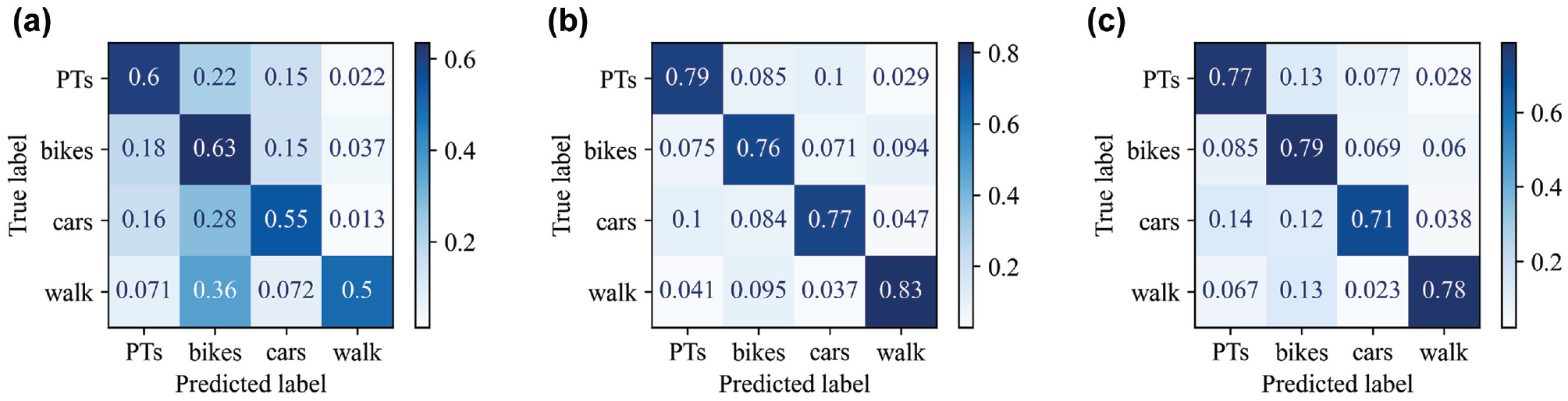
Confusion matrices for the three models (single runs). (a) Multinomial logit regression. (b) Extreme gradient boosting. (c) Random forest.

Interpretability

The results from the ML-based models and particularly the XGBoost model look promising so far; the gap in performance compared to the MNL model is greater than 20%. Yet, the key advantage of these models, their complexity, is also their largest disadvantage. They learn advanced patterns and excel at predicting; however, it becomes seemingly impossible to back-track the model’s decision-making steps. While it is neither feasible nor practical to look at each decision made in the training process, one approach that has seen a rise in interest is SHAP.

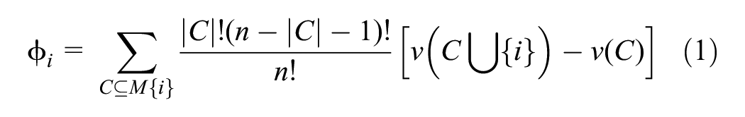
SHAP ( 31 ) was developed based on the idea that there is a need to be able to explain the contribution of each feature to the predictions made. Essentially, a Shapley value assesses the mean relative deviation in output if a feature is excluded compared to when it is included, in all possible combinations. The corresponding mathematical formulation is shown in Equation 1, where $ϕ_{i}$ is the Shapley value of a feature $i$ , $C$ is a coalition of $n$ features (of all $N$ features $M$ ), and $v (M)$ is the model output. Lundberg and Lee ( 31 ) proposed to formulate a function that combines Shapley values of all features $M$ in an additive manner, as shown in Equation 2 where $z'$ is 1 if a feature is present, else 0 ( 11 ). Three key advantages of SHAP are that it provides accurate and consistent results while being able to deal with missing input values:

ϕ_{i} = \sum_{C \subseteq M {i}} \frac{| C |! (n - | C | - 1)!}{n!} [v (C ⋃ {i}) - v (C)]

(1)

g (z') = ϕ_{0} + \sum_{i = 1}^{N} ϕ_{i} z'_{i}

(2)

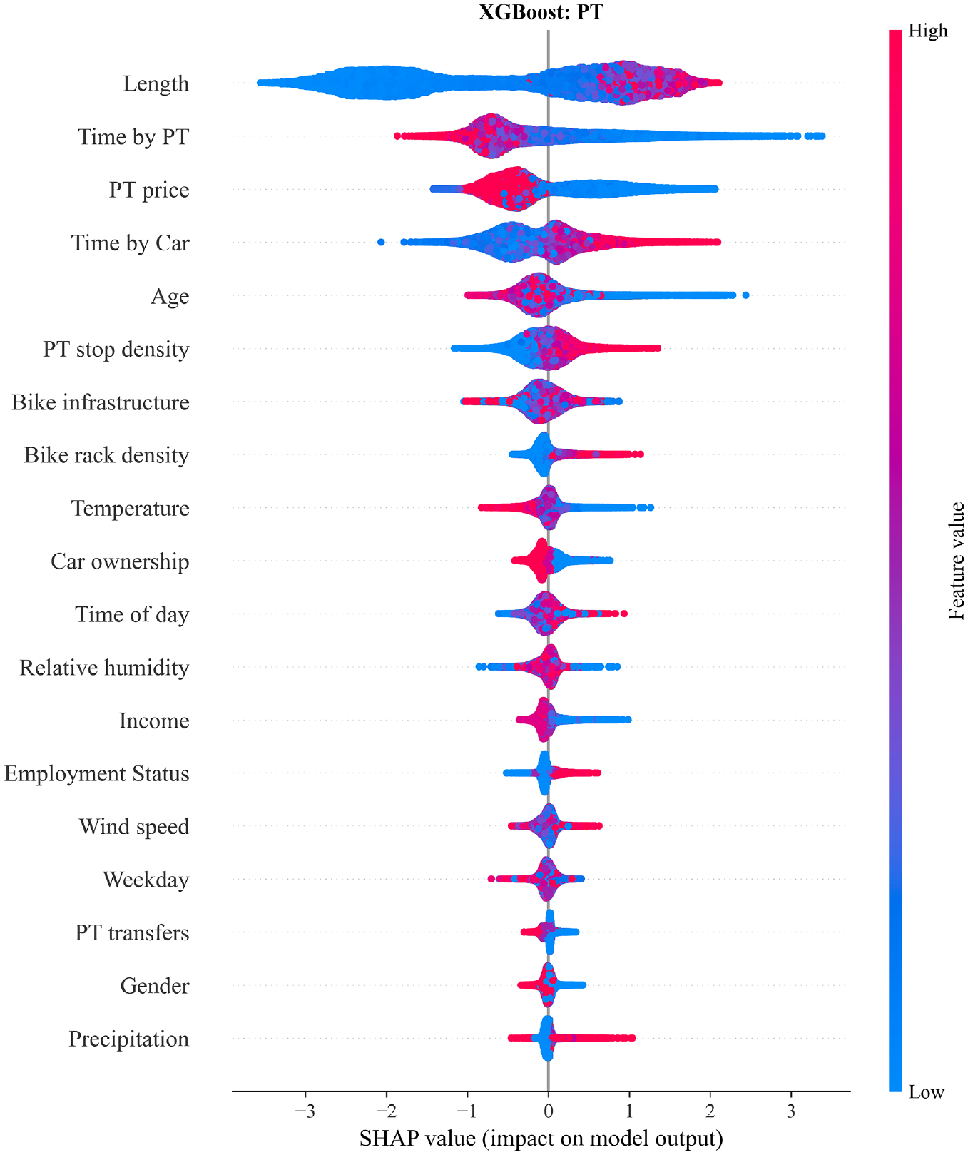
In this section, only the interpretability of the best-performing model, XGBoost, will be explored in depth, and as such a SHAP analysis can be performed for the other models in the same manner. Figure 4 shows the average magnitude of each feature’s SHAP values (features with the highest contribution at the top). For instance, length is by far the most important indicator of the mode, followed by PT price and time by car, and time by PT. This is in line with mode choice literature, for example, Tamim Kashifi et al. ( 13 ) also found the trip length to be the most important attribute, and Wang et al. ( 14 ) found length and travel time to be most indicative. PT price is rarely considered in the literature; however, estimated travel times are frequently considered and found to be among the most contributing features ( 5 , 10 ). Overall, temperature and age are the only relevant weather-related and sociodemographic features, respectively. The variable age is found to be most important among the sociodemographic data by Cheng et al. ( 5 ), and right after travel time by Richards and Zill ( 15 ); neither of the two considers length or PT price. It is noted that the RF model had the same top eight features with only two shifted by a spot (age, PT stop density), indicating consistency across models and fostering the trustworthiness of SHAP values.

Figure 4.

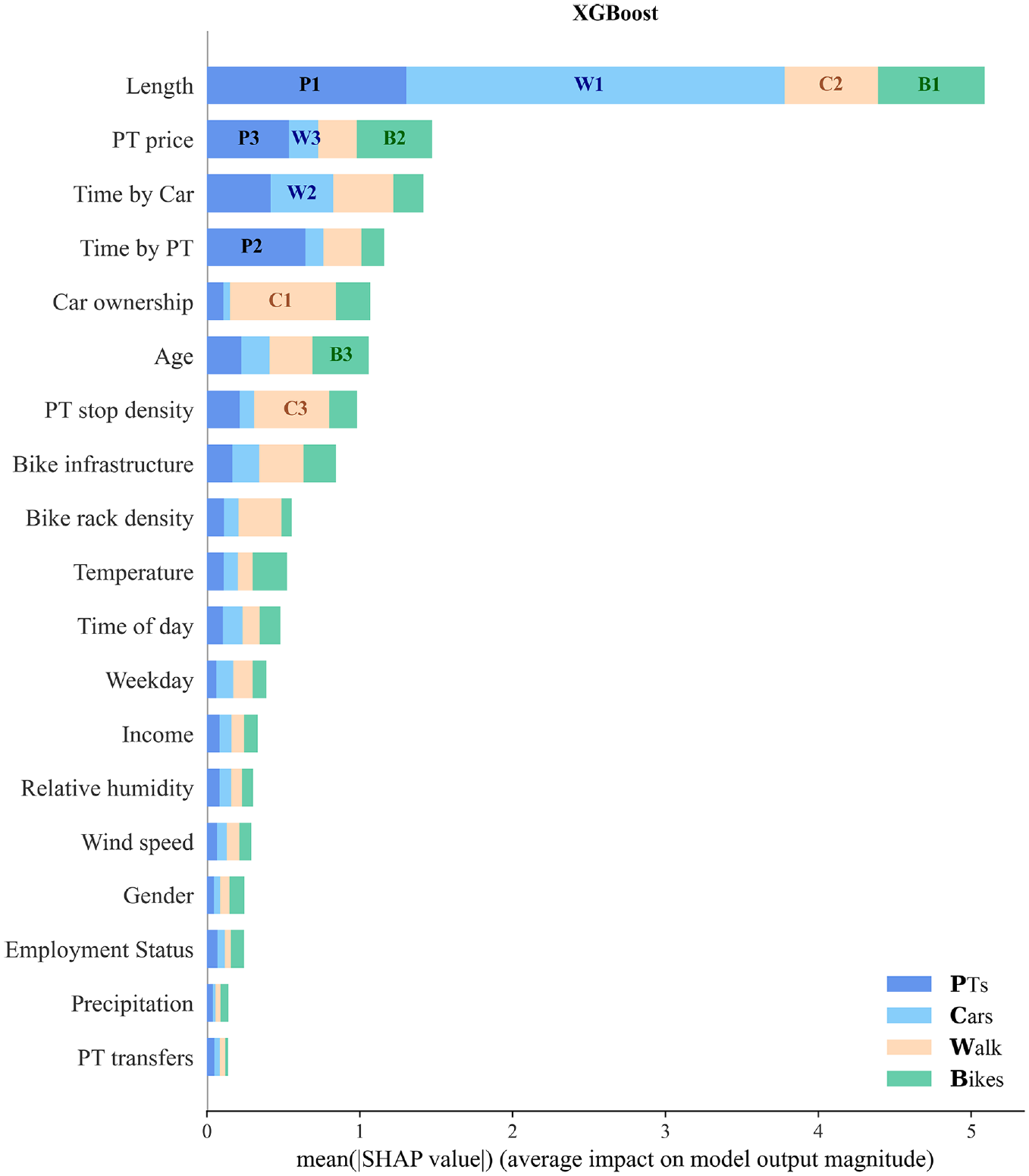
The contribution of each feature to the output class (mode) by mean SHAP (SHapley Additive exPlanations) value for the extreme gradient boosting (XGBoost) model at an (i) aggregate level: total width, that is, most impactful feature at the top, and (ii) individual level for each mode: denoted by the colors, where the numbers indicate the three features that contribute most to a mode.

So far, we have explored the overall impact of each feature. However, we can also see each feature’s relative contribution to each mode, as shown by the colors in Figure 4. The numbers denote which three features affect each mode prediction most. For instance, the length contributes most to walk predictions (light blue), as denoted by “W1.” In addition, we can also look at how exactly features’ values affect each mode classification. The impacts of features on individual modes are rarely discussed in the context of ML for transportation mode choice, yet it is essential when discussing its potential use for behavioral analyses. Such information is conveyed in Figures 5 –9, where the features are ordered by relative contribution (analogous to the numbers in Figure 4). The high values (upper end of the color scale) reflect a high value in the input data. Categorical variables are encoded as shown in Table 1, for example, 0 for Monday and 6 for Sunday.

Figure 5.

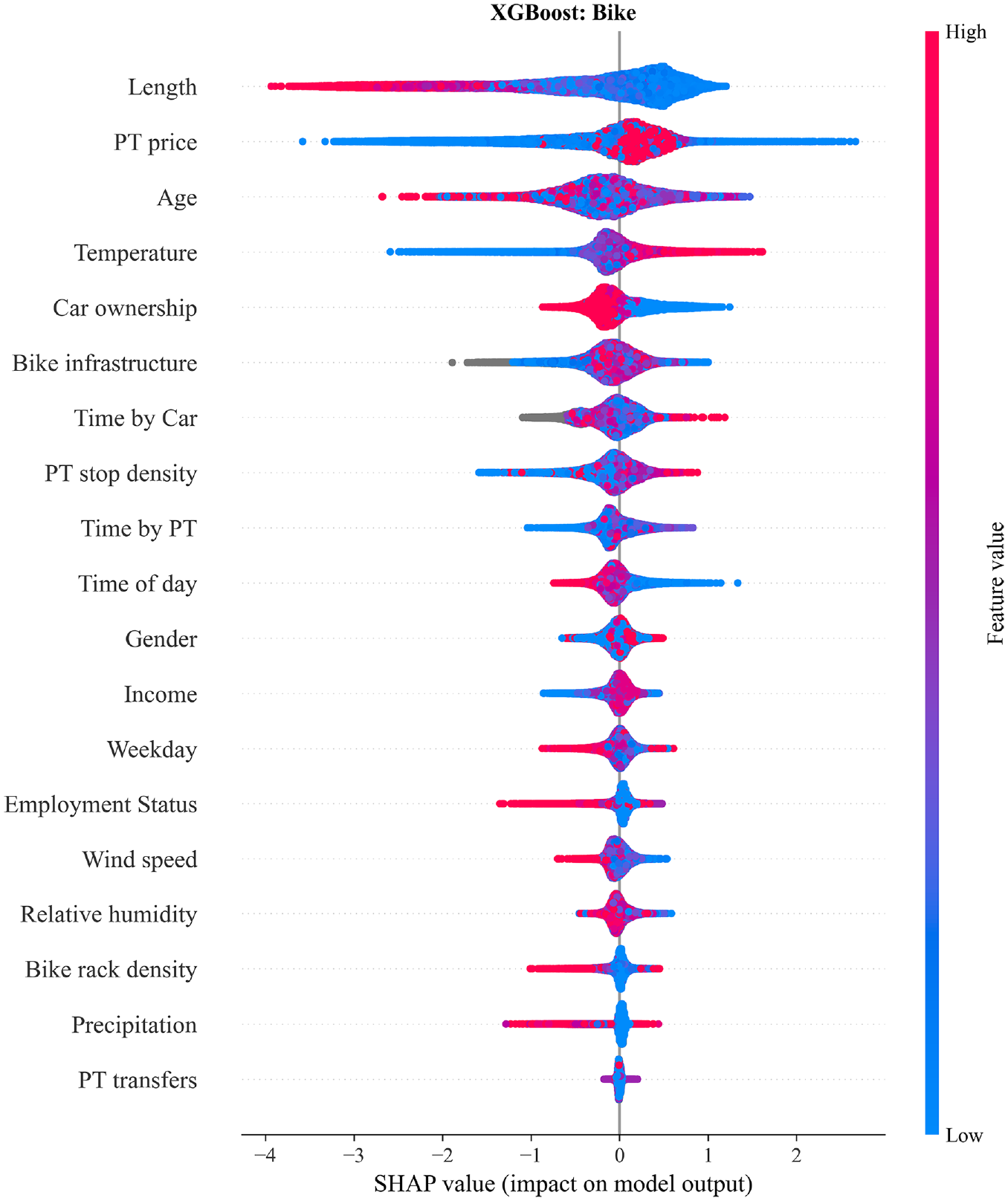
The impact of each feature on the bike class in the form of SHAP (SHapley Additive exPlanations) value dependencies for the extreme gradient boosting (XGBoost) model. High and low correspond to the features’ highest/lowest values. Gray dots represent missing values.

Figure 6.

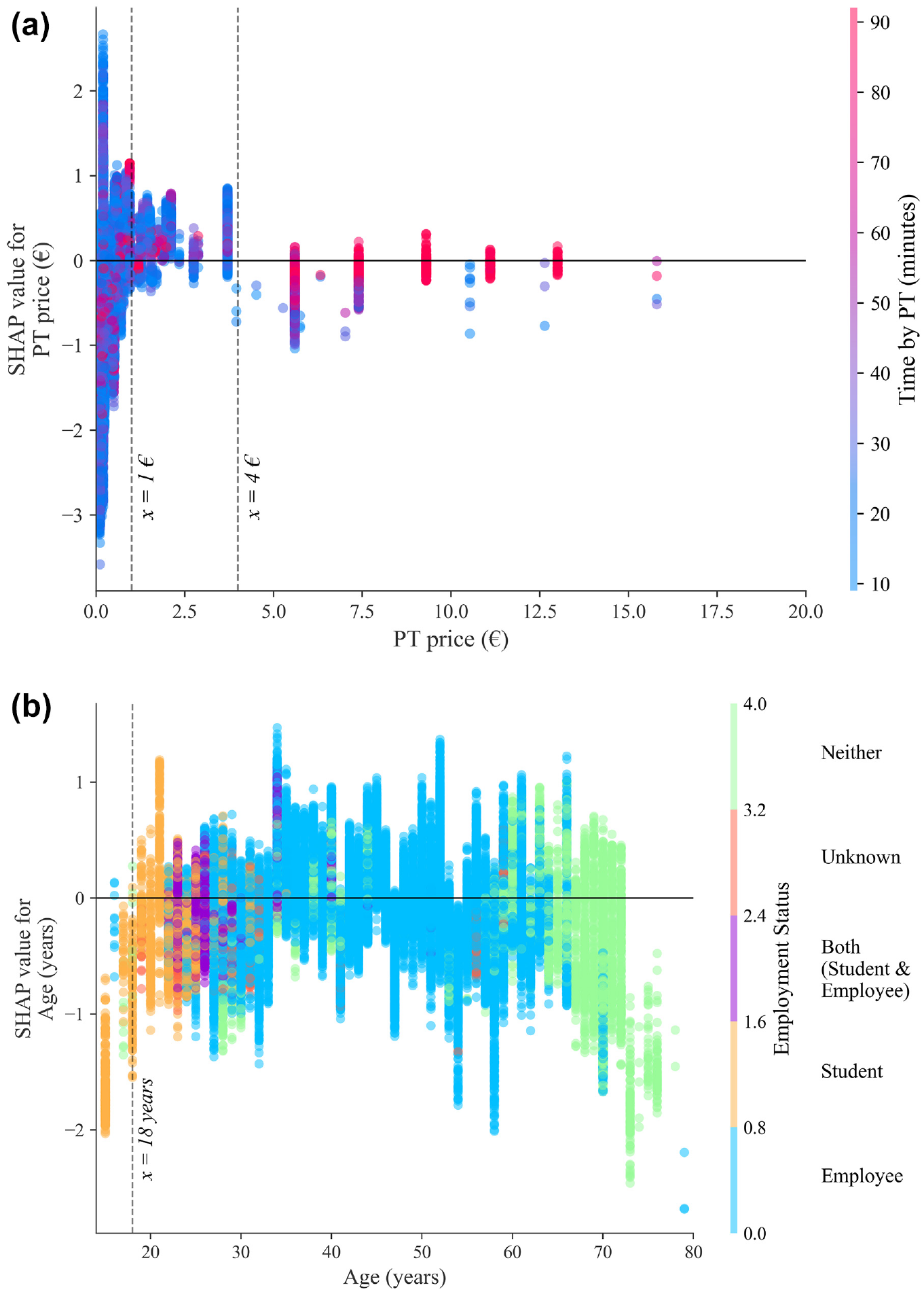
SHAP (SHapley Additive exPlanations) dependency plots for selected variables for the output class bike. (a) SHAP values for the class bike for the feature public transport (PT) price, colored by PT time. (b) SHAP values for the class bike for the feature age, for the respective employment status.

Figure 7.

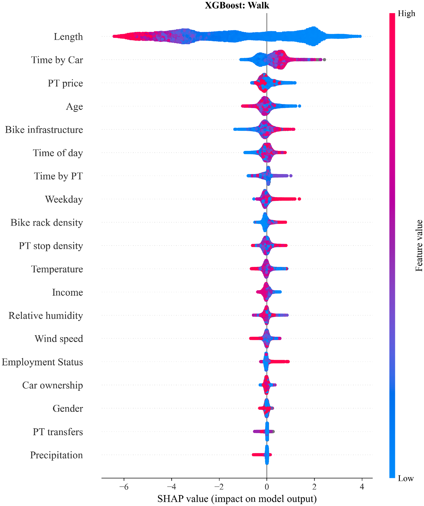
The impact of each feature on the walk class in the form of SHAP (SHapley Additive exPlanations) value dependencies for the extreme gradient boosting (XGBoost) model. High and low correspond to the features’ highest/lowest values. Gray dots represent missing values.

Figure 8.

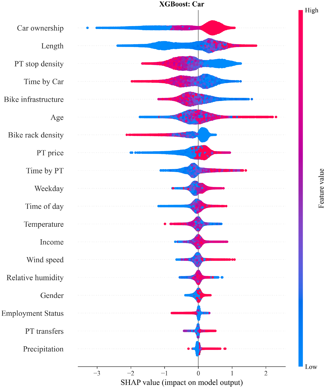
The impact of each feature on the car class in the form of SHAP (SHapley Additive exPlanations) value dependencies for the extreme gradient boosting (XGBoost) model. High and low correspond to the features’ highest/lowest values.

Figure 9.

The impact of each feature on the public transport (PT) class in the form of SHAP (SHapley Additive exPlanations) value dependencies for the extreme gradient boosting (XGBoost) model. High and low correspond to the features’ highest/lowest values.

Starting with Figure 5, the features length, PT price, age, and temperature contribute most to bike predictions. The length is intuitive as very short or long trips will typically not be made by bike. Similarly, temperature and bike infrastructure (in sixth place) were also expected to be features that have high contribution; Winters et al. ( 32 ) made the same observations in a SP survey. People are less willing to cycle in cold, icy conditions, if the trip length is high and if there is no designated cycling infrastructure. The SHAP values of the PT price are not linearly distributed. This was further investigated using a partial dependence plot (Figure 6a), which reveals that for low to medium values (around €1–€4, as shown by the dashed lines) the SHAP values are positive (cycling is more likely). For higher prices, people tend to not cycle when the corresponding time by PT is low.

The age variable has a very uneven color distribution (no easily identifiable trend), yet Figure 6b shows that young people (particularly university students) are on average more likely to cycle. For older age groups, who are almost entirely retired, there is, on average, a negative SHAP value. Across the other age groups, it is difficult to identify a relationship. Interestingly, precipitation, wind, and relative humidity have little impact on the model output, while many occasional or leisure cyclists would dispute that. Nonetheless, similar observations have been made by Tamim Kashifi et al. ( 13 ). The effects of temperature and bike infrastructure are both positive at higher feature values and support the findings of Hull and O’Holleran ( 33 ).

Walking is by far most affected by length, as walks are typically short. The time by car, PT price, and age follow, as shown in Figure 7. The mean absolute SHAP value of length is 2.4, while the next most important feature only has a mean SHAP value of 0.3; for the other modes, this gap does not exceed a magnitude of 0.4. The gray section for time by car with high SHAP values represents trips where no estimated time by car was available, that is, for very short trips or when there is no road available, for example, in a park. Furthermore, a high time by car and time by PT discourage walking. For older individuals, the age will have a more negative SHAP value, that is, it contributes negatively to the walk prediction. For the PT price we observe that for a price range of around €1.5–€4 the walking SHAP values are negative. As the price of a regular short–medium distance single ticket is either €1.8 or €3.6, this pattern likely reflects inner-city trips, where walking would be inconvenient.

The choice of the car is influenced most by car ownership and length, followed by the PT stop density and time by car (see Figure 8). For car ownership, a high value of 2 indicates that a person has access to a car; therefore, the user is more likely to take a car, resulting in the positive SHAP value. The opposite is the case for people without a car, denoted by 0. If it is not known if a car is available, that is, 1, the SHAP values remain slightly negative. The remaining three top features follow clear monotone trends, for example, a high PT stop density discourages car use, as driving is inconvenient in the city center because of a lack of parking and traffic. A high time by car and low length increase the contribution of these features to the overall prediction being “Car.”

Similarly, the four features with the highest SHAP values for “PT” also follow linear trends (Figure 9). A high length contributes positively to PT predictions, along with a low time by PT and a low PT price. A high time by car also encourages PT trips, yet time by car correlates with length to an extent, as shown in Figure 10. Such trips make cycling and walking unattractive options, and if the time by car is low in comparison to the time by PT, PT is less likely to be the mode of choice.

Figure 10.

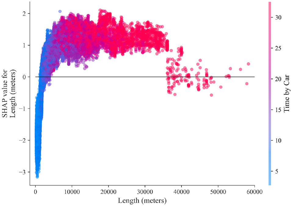
SHAP (SHapley Additive exPlanations) dependence plot for public transport for the feature length for the extreme gradient boosting model.

Thus far we have been looking at the average values across the entire dataset. It is also possible to investigate to what extent individual features affect the classification output of an individual prediction. In brief, for each mode, the SHAP values of each feature (positive as well as negative) are summed up to an overall SHAP value. The mode with the highest sum indicates the predicted label. An example of a correctly predicted PT trip is shown in Figure 11, which illustrates how each input feature contributed to the overall result. For instance, an individual does not have access to a car, has a monthly PT pass, is 57 years old, and makes a 6.1 km trip on a Sunday around 16:00. In this case, the attributes that contribute most (the ones with the highest absolute SHAP values) are as follows: the PT price is very low at €0.16 (because of the monthly PT pass), the trip length (6.1 km) is a typical PT trip and atypical walking trip, and the lack of access to a car makes it an unlikely choice. This explains the PT classification, as this is the mode with the highest sum of individual SHAP values (denoted in bold at the top of the figure).

Figure 11.

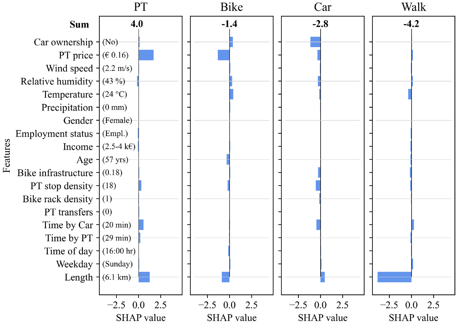
Evaluation of the SHAP (SHapley Additive exPlanations) values of a single predicted public transport (PT) trip for the extreme gradient boosting model. The magnitude of each bar displays the contribution of that feature’s value to the corresponding mode’s overall SHAP value (the sum).

Sensitivity Analysis

Now that we have found the best-performing model for mode choice prediction and have shown that it is explainable, we will use a sensitivity analysis to shed light on factors that could hinder its implementation in practice: lack of data sources, reduced availability of TRP data, and uncooperative users or fully passive TRP data. The results of the previous models (which is used as a baseline) and the results obtained when leaving out certain input feature groups, altering the dataset size, and selecting uninvolved users are summarized in Table 3.

In this paper, a total of 22 features (19 excluding collinear features) are used, yet such a wide range of variables may not always be available. Some of the data can be obtained as open-source, while other features such as car ownership have to be collected. It is well-known that ML models tend to perform best with more features, as confirmed by Richards and Zill ( 15 ) for transportation mode choice prediction using CRP data. It is of interest to know how much the model performance may decrease when different categories of data are not available. It is found that the absence of survey-based data (sociodemographic data, PT monthly pass, and car ownership) has the biggest impact: a 3% reduction in mean accuracy for XGBoost and RF. This is realistic, as PT price, car ownership, and age highly contribute to the predictions (Figure 4); nonetheless, both models still surpass the MNL by far. Removing the weather data or, interestingly, the alternative travel times has the lowest effect. On the whole, the XGBoost model is less affected by the removal of feature groups compared to the RF. The MNL demonstrates distinctly different (albeit worsened) patterns in comparison to the XGBoost and RF models. If only the data taken directly from the travel diaries (length, time of day, weekday) is used, this leads to an accuracy of around 50% for all three models. This shows the importance of the length variable. Furthermore, it was tested whether the inclusion of the previously excluded collinear variables affects the model performance. As expected, they either have no effect or worsen the performance.

In contrast, it may occur that a wide range of features is available but that the sample size is relatively small. In ML, this can lead to critical issues, as sufficient data is required to accurately learn travel behavior patterns. It was tested how much the accuracies decrease if less training data is used. Because of the relatively even modal split, a fixed number of trips per mode was selected: 10,000, 3000, and 700. It is noted that no special techniques were used to enhance the models’ abilities in learning from a small training dataset. From Table 3 it is evident that the performance of the XGBoost and RF models is notably reduced (for 700 trips per mode: XGBoost by 10.7% and RF by 13.0%) while still outperforming the MNL (3.2% drop) with respect to overall accuracy. It is evident that the ML approach strongly benefits from a high amount of training data. This initially seems drastic, yet with TRP data, it is easier than ever to scale up the size of the dataset by extending the tracking period (or acquiring more users).

Lastly, the use of semi-passive instead of fully passive travel diaries—where there is no sort of user interaction or validation—improves the accuracy. The latter is tested by selecting users from the study who were known to not have corrected the draft diaries generated by the smartphone-tracking app. Thus far, the final model had only used data from committed users that frequently correct erroneous recordings, yet when using such “fully passive” data, all models’ performance dropped: XGBoost by 2.6%, RF by 3.4%, and MNL by 4.1%. This illustrates the importance of incentivizing users to validate and rectify trip detection errors, which are often not fixable during post-processing, therefore impeding pattern recognition by the mode choice models.

Conclusions

In this paper, we presented the application of two ML models to a TRP dataset to predict transportation mode choice. These two selected models have performed well on SP and self-reported CRP data, yet their performance and explainability have not previously been studied for TRP data. The XGBoost model, in particular, and the RF model outperformed the conventional MNL model. The interpretability of the best-performing model was investigated thoroughly using SHAP values. It was found that trip length, PT price, and estimated travel times by car and PT contribute most to the overall mode predictions. We also identified the key factor for each individual mode: trip length was most important for all modes except for car, where car ownership contributed slightly more. Lastly, a brief sensitivity analysis gave insight into issues that might be frequently encountered in practice.

The use of TRP data compared to CRP data promises precise locations and timestamps, a wide range of potential features, and circumvents the issue of trip underreporting. Yet, TRP data is subject to the reliability and commitment of users and good data processing to reduce errors in tracking. We found that high user involvement can improve the ML models’ results. For completeness, we would like to point out the limitations of our study. Firstly, we have not performed a sensitivity analysis of how changing individual features affects the model output. This could reveal relevant insights on model robustness. Secondly, with regards to data quality, we only considered the lack of user validation, but no factors related to the recording device, that is, the smartphone.

In future studies, a comparative analysis of TRP, CRP, and SP data would be worth exploring. Thus far, only the latter two have been compared ( 12 ). Altogether, the findings in this paper about the accuracy and interpretability of ML models for TRP data aid in the evaluation and analysis of future TRP studies, while also shedding light on the travel behavior in the case study area of Munich, Germany.

Footnotes

Author Contributions

The authors confirm contribution to the paper as follows: study conception and design: V. Dahmen, S. Weikl; data collection: V. Dahmen, K. Bogenberger; analysis and interpretation of results: V. Dahmen, S. Weikl; draft manuscript preparation: V. Dahmen, S. Weikl, K. Bogenberger. All authors reviewed the results and approved the final version of the manuscript.

Declaration of Conflicting Interests

The author(s) declared no potential conflicts of interest with respect to the research, authorship, and/or publication of this article.

Funding

The author(s) disclosed receipt of the following financial support for the research, authorship, and/or publication of this article: The research presented is supported by the TUM Georg Nemetschek Institute Artificial Intelligence for the Built World. The authors would like to thank the TUM Think Tank for their financial and organizational support in the genesis of the Mobilität.Leben project.

ORCID iDs

Victoria Dahmen

Simone Weikl

Klaus Bogenberger

References

Barff

Mackay

Olshavsky

R. W.

A Selective Review of Travel-Mode Choice Models. Journal of Consumer Research, Vol. 8, No. 4, 1982, pp. 370–380. http://www.jstor.org/stable/2489024

Reck

D. J.

Martin

Axhausen

K. W.

Mode Choice, Substitution Patterns and Environmental Impacts of Shared and Personal Micro-Mobility. Transportation Research Part D: Transport and Environment, Vol. 102, 2022, p. 103134. https://doi.org/10.1016/j.trd.2021.103134

Hagenauer

Helbich

A Comparative Study of Machine Learning Classifiers for Modeling Travel Mode Choice. Expert Systems with Applications, Vol. 78, 2017, pp. 273–282. https://doi.org/10.1016/j.eswa.2017.01.057

García-García

J. C.

García-Ródenas

López-Gómez

J. A.

Martín-Baos

J. A.

A Comparative Study of Machine Learning, Deep Neural Networks and Random Utility Maximization Models for Travel Mode Choice Modelling. Transportation Research Procedia, Vol. 62, 2022, pp. 374–382. https://doi.org/10.1016/j.trpro.2022.02.047

Cheng

Chen

De Vos

Lai

Witlox

Applying a Random Forest Method Approach to Model Travel Mode Choice Behavior. Travel Behaviour and Society, Vol. 14, 2019, pp. 1–10. https://doi.org/10.1016/j.tbs.2018.09.002.

Lee

Mulrow

Haboucha

C. J.

Derrible

Shiftan

Attitudes on Autonomous Vehicle Adoption using Interpretable Gradient Boosting Machine. Transportation Research Record: Journal of the Transportation Research Board, Vol. 2673, No. 11, 2019, pp. 865–878. https://doi.org/10.1177/0361198119857953

Prelipcean

A. C.

Susilo

Y. O.

Gidófalvi

Collecting Travel Diaries: Current State of the Art, Best Practices, and Future Research Directions. Transportation Research Procedia, Vol. 32, 2018, pp. 155–166. https://doi.org/10.1016/j.trpro.2018.10.029

Thomas

Geurs

K. T.

Koolwaaij

Bijlsma

Automatic Trip Detection with the Dutch Mobile Mobility Panel: Towards Reliable Multiple-Week Trip Registration for Large Samples. Journal of Urban Technology, Vol. 25, No. 2, 2018, pp. 143–161. https://doi.org/10.1080/10630732.2018.1471874.

Montini

Prost

Schrammel

Rieser-Scḧussler

Axhausen

Comparison of Travel Diaries Generated from Smartphone Data and Dedicated GPS Devices. Transportation Research Procedia, Vol. 11, pp. 227–241. https://doi.org/10.1016/j.trpro.2015.12.020

10.

Zhao

Yan

Van Hentenryck

Prediction and Behavioral Analysis of Travel Mode Choice: A Comparison of Machine Learning and Logit Models. Travel Behaviour and Society, Vol. 20, 2020, pp. 22–35. https://doi.org/10.1016/j.tbs.2020.02.003

11.

Pineda-Jaramillo

Arbeláez-Arenas

Assessing the Performance of Gradient-Boosting Models for Predicting the Travel Mode Choice Using Household Survey Data. Journal of Urban Planning and Development, Vol. 148, No. 2, 2022, p. 04022007. https://doi.org/10.1061/(ASCE)UP.1943-5444.0000830

12.

Teng

Understanding Influencing Factors of Travel Mode Choice in Urban-Suburban Travel: A Case Study in Shanghai. Urban Rail Transit, Vol. 9, No. 2, 2023, pp. 127–146. https://doi.org/10.1007/s40864-023-00190-5

13.

Tamim Kashifi

Jamal

Samim Kashefi

Almoshaogeh

Masiur Rahman

Predicting the Travel Mode Choice With Interpretable Machine Learning Techniques: A Comparative Study. Travel Behaviour and Society, Vol. 29, 2022, pp. 279–296. https://doi.org/10.1016/j.tbs.2022.07.003

14.

Wang

Zhao

Predicting Travel Mode Choice With 86 Machine Learning Classifiers: An Empirical Benchmark Study. In Transportation Research Board 99th Annual Meeting. Washington, DC, USA, 2020, pp. 279–296. https://api.semanticscholar.org/CorpusID:232333536

15.

Richards

M. J.

Zill

J. C.

Modelling Mode Choice With Machine Learning Algorithms. In Proceedings of the Australasian Transport Research Forum, ATRF. Canberra, Australia, 2019, pp. 1–15.

16.

Wang

Ross

C. L.

Machine Learning Travel Mode Choices: Comparing the Performance of an Extreme Gradient Boosting Model with a Multinomial Logit Model. Transportation Research Record: Journal of the Transportation Research Board, Vol. 2672, No. 47, 2018, pp. 35–45. https://doi.org/10.1177/0361198118773556

17.

Buijs

Koch

Dugundji

Applying Transfer Learning and Various ANN Architectures to Predict Transportation Mode Choice in Amsterdam. Procedia Computer Science, Vol. 184, 2021, pp. 532–540. https://doi.org/10.1016/j.procs.2021.03.067

18.

Bhuiya

M. M. R.

Hasan

M. M. U.

Keellings

D. J.

Mohiuddin

Application of Machine Learning Classifiers for Mode Choice Modeling for Movement-Challenged Persons. Future Transportation, Vol. 2, No. 2, 2022, pp. 328–346. https://doi.org/10.3390/futuretransp2020018

19.

Loder

Cantner

Adenaw

Siewert

Goerg

Lienkamp

Bogenberger

A Nation-Wide Experiment: Fuel Tax Cuts and Almost Free Public Transport for Three Months in Germany – Report 1 Study Design, Recruiting and Participation, 2022. https://doi.org/10.48550/arXiv.2206.00396

20.

Dahmen

Álvarez Ossorio Martínez

Loder

Bogenberger

Making Large-Scale Semi-Passive GPS Travel Diaries Valuable: A Quality Enhancement Method. In Transportation Research Board 103rd Annual Meeting. Washington, DC, USA, 2024, pp. 1–19. https://doi.org/10.13140/RG.2.2.28580.04487/1

21.

Friedman

J. H.

Greedy Function Approximation: A Gradient Boosting Machine. The Annals of Statistics, Vol. 29, No. 5, 2001, pp. 1189–1232. https://doi.org/10.1214/aos/1013203451

22.

Joshi

A. V.

Machine Learning and Artificial Intelligence, 2nd edn. Springer International Publishing, Redmond, WA, 2023. https://doi.org/10.1007/978-3-031-12282-8

23.

Pineda-Jaramillo

J. D.

A Review of Machine Learning (ML) Algorithms Used for Modeling Travel Mode Choice. DYNA, Vol. 86, No. 211, 2019, pp. 32–41. https://doi.org/10.15446/dyna.v86n211.79743

24.

Deutscher Wetterdienst. Klimadaten Deutschland -Monatsund Tageswerte (Archiv), 2023. https://opendata.dwd.de/climate_environment/CDC/observations_germany/climate/hourly/. Last Accessed July 20, 2023.

25.

OpenStreetMap contributors. Planet dump retrieved from https://planet.osm.org . https://www.openstreetmap.org,2017.

26.

TomTom. Routing API and Extended Routing API, 2023. https://developer.tomtom.com/routing-api/documentation/routing/calculate-route. Last Accessed May 27, 2023.

27.

Software Freedom Conservancy. OpenTripPlanner 2, 2023. https://docs.opentripplanner.org/en/v2.2.0/. Last Accessed July 20, 2023.

28.

Freedman

Pisani

Purves

Statistics (International Student Edition), 4th edn. WW Norton & Company, New York, NY, 2007.

29.

Sekhar

C. R.

Minal Madhu

Mode Choice Analysis Using Random Forrest Decision Trees. Transportation Research Procedia, Vol. 17, 2016, pp. 644–652. https://doi.org/10.1016/j.trpro.2016.11.119

30.

The Scikit-Learn Development Team. Metrics and scoring: quantifying the quality of predictions, 2023. https://scikit-learn.org/stable/modules/model_evaluation.html#accuracy-score. Last Accessed November 22, 2023.

31.

Lundberg

S. M.

Lee

S. -I.

A Unified Approach to Interpreting Model Predictions. Advances in Neural Information Processing Systems, Vol. 30, pp. 4765–4774.

32.

Winters

Davidson

Kao

Teschke

Motivators and Deterrents of Bicycling: Comparing Influences on Decisions to Ride. Transportation, Vol. 38, No. 1, 2011, pp. 153–168. https://doi.org/10.1007/s11116-010-9284-y

33.

Hull

O’Holleran

Bicycle Infrastructure: Can Good Design Encourage Cycling?

Urban, Planning and Transport Research, Vol. 2, No. 1, 2014, pp. 369–406. https://doi.org/10.1080/21650020.2014.955210

Interpretable Machine Learning for Mode Choice Modeling on Tracking-Based Revealed Preference Data