Sage Journals: Discover world-class research

Abstract

Commuting is a major contributor to $C O_{2}$ emissions from passenger transportation. This study examines the potential of commuting demand management (CDM) by analyzing within-person variability in commuting mode choices. We utilized GPS tracking data to monitor the commuting trips of 129 participants in Germany from September 2022 to August 2023. On average, each participant recorded 10 months of data with 106 trips between their “main home” and “main work” location. Our findings indicated that participants typically use three different main modes for their commuting trips. The Herfindahl–Hirschmann index and the difference between the primary and alternative modes revealed differences in the modal stability among commuters, with some showing high variability and others low. Factors such as gender, possession of a driver’s license, and economic status appeared to influence this variability. We further categorized individuals into commuter modal types (active, public, private motorized) per month using k-means clustering. After 5 months, 71.1% of commuters remained in their original modal type cluster (95% CI: 63.6% to 79.4%). However, by the 10-month mark, this figure had decreased to 58.9% (95% CI: 48.8% to 71.0%). This observed variability in commuting mode choices suggests opportunities for CDM. By designing policies that promote the use of sustainable modes already adopted by commuters, CDM could effectively increase the modal share of these environmentally friendly options.

Keywords

mode choice travel behavior demand management

The transportation sector is responsible for a significant share of climate-relevant emissions in both Germany and the United States, accounting for 20% and 28% of total emissions, respectively ( 1 , 2 ). Commuting contributes to more than one-fifth of emissions from passenger transportation ( 3 ). Therefore, interest in effective measures to decarbonize commuting has increased in recent years ( 4 , 5 ). Given that travel by private automobile is the most emission-intensive mode of transportation, efforts to promote sustainable modes of transportation are a primary focus ( 6 , 7 ). However, when attempting to describe and model commuter travel behavior, the focus is predominantly between individuals rather than within individuals. As habits drive mode choice by automated cognitive processes ( 8 ), intrapersonal behavior is assumed to be rather stable. To understand the potential of policies to induce individuals to change their travel mode, it is promising to investigate the variability they already exhibit in their mode choice. Heinen and Ogilvie demonstrated that commuters with greater modal variability were more likely to increase active mode use when a new walking and biking path was built ( 9 ).

Table 1 provides an overview of the literature on within-person mobility variability. Different outcomes have been studied, including (commuter) mode choice, route choice, destination choice, departure choice, and trip frequency. Most studies find a significant share of individuals who exhibit instability in their mobility patterns. Constraints can explain some of the variability that individuals exhibit, for example, financial constraints ( 10 ) or mode availability ( 11 ). In general, there have been two dominant approaches to studying mobility variability: travel diary surveys, often with a larger sample size and a period of 1 to 6 weeks, and GPS tracking data. Using GPS tracking data is promising since it reduces the burden on the respondents and thus allows for the collection of longer-term data ( 12 ). However, previous studies of modal variability drawing on GPS tracking data have mainly studied shorter periods, with the notable exception of Hong et al. ( 13 ).

Table 1.

Literature on Intraperson Mobility Variability

Authors	Data	N	Outcome	Indicators	Findings
Arifin and Axhausen ( 14 )	One-week GPS tracking	93	Commuter mode and route choice	Number of main modes/routes	17% used more than one commuting main mode, 80% of car users used multiple routes
Chatterjee et al. ( 11 )	North Bristol Commuter Panel	1,947	Commuter mode choice	Mode use frequencies (clusters)	70% of commuters are unimodal, around 25% changed their commuting pattern 3 months later
Cherchi and Cirillo ( 15 )	Six-week travel diary survey (Mobidrive)	203	Mode choice	Preferences for travel time and cost	Preferences were stable over weeks, inertia effect for mode choice
Chowdhury et al. ( 16 )	Four-week tracking data (Dutch Mobile Mobility Panel)	442	Destination choice, departure time, and mode choice	Spatial repetition index, temporal repetition index	Higher variability for less often visited destinations
Crawford ( 17 )	Seven-day travel diary over 19 years (National Travel Survey)	118,194	Frequency of travel, spatial and temporal variability	Cluster membership	Four distinct groups of commuters were identified with different types and levels of variability
Hatcher and Mahmassani ( 18 )	Two-week travel diaries	164	Trip timing and route choice for commuting trips	Median switching, day-to-day switching	Departure times are more variable than routes
Heinen and Chatterjee ( 19 )	Seven-day travel diary from 2010 (National Travel Survey)	19,072	Modal variability	Number of modes, percentage of travel by mode, primary/secondary mode, difference in share between primary and secondary mode, Herfindahl–Hirschmann index	69% of participants are multimodal; mobility constraints limit modal variability
Hong et al. ( 13 )	GPS tracking (GC & MOBIS)	3,414	Mode choice and destination choice	Radius of gyration, jump length, location visitation frequency, activity space	Typically, individuals are observed to have around 15 mode–location choices as a conserved quantity
Pas and Koppelman ( 10 )	Five-day travel survey	145	Trip frequency	Mean intrapersonal variance in daily trip generation rates	Financial and role-related constraints reduce variability
Raux et al. ( 20 )	Seven-day travel diary	707	Number of trips/tours, time allocation, activity sequence	Between-day and within-day within-person variability	Sociodemographic variables cannot describe intrapersonal variability accurately
Schlich ( 21 )	Six-week travel diary (Mobidrive)	361	Activity pattern	Similarity index (Hanson), similarity index (Pas), similarity index (Clarke/Jones)	Variability is higher on nonworking days
Shen et al. ( 22 )	Seven-day GPS tracking	102	Commute travel time, location, mode and route choice	Number of unique occurrences	Variability in time is the greatest
Streit et al. ( 23 )	One-week multiyear travel diary (MOP)	2,000	Mode choice, activities	Multimodal indicator, trip chain measure, standard deviation, dispersion	Young individuals are more likely to be multimodal
Susilo and Axhausen ( 24 )	Six-week travel diary (Mobidrive and Thurgau)	547	Individual daily activity–travel–location patterns	Herfindahl–Hirschmann index	Non-mandatory activities are less repetitive in their activity–travel–location combinations
Tarigan et al. ( 25 )	Six-week travel diary (Mobidrive)	136	Trip frequency, activity duration, travel time and distance		Individuals from one-worker households have greater variability
Costa et al. ( 26 )	GPS tracking	172	Departure time, mode and line choice, trip duration	Similarity index	High regularity of commuting behavior

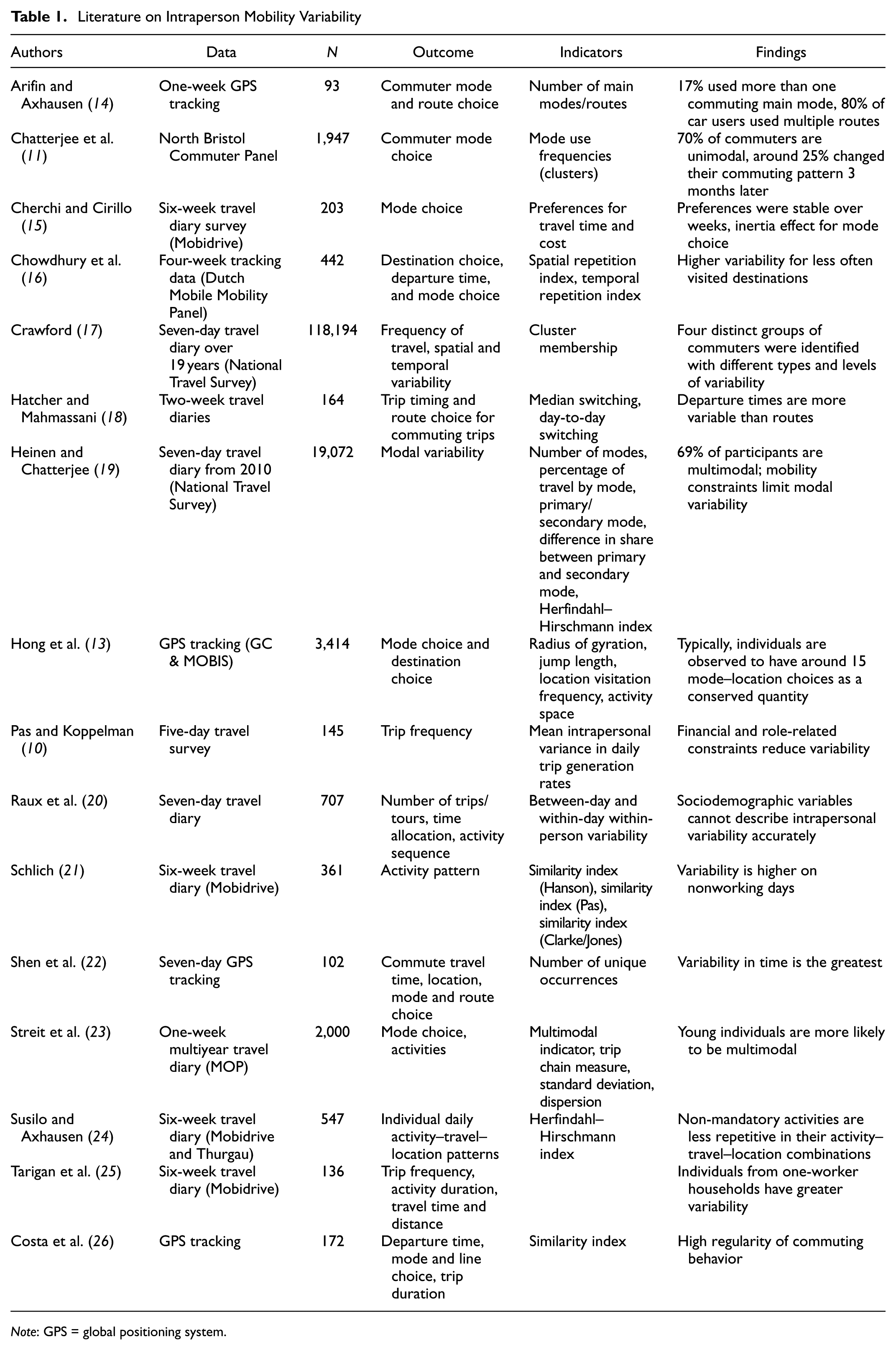
Note: GPS = global positioning system.

In this paper, we explore intrapersonal variability in commuter mode choice using a year-long labeled GPS panel dataset. To the best of our knowledge, this is the first study to use 12 months of GPS tracking data to specifically describe and analyze commuting behavior. We investigate the stability of mode choice for the same trip (home to work) and identify factors influencing individual variability. Employing various modeling approaches, we analyze all trips during the observation period and segment the data by user-month. Our analyses provide insights into commuter flexibility and the potential for carbon savings through appropriate policies. The results are relevant to the concept of commuting demand management (CDM), that is, policies that seek to influence commuting behavior, both from a policy and a business perspective.

The paper is organized as follows: first, the study design and data collection are described. Then, the data processing steps are outlined, as well as the methodology. In the results section, we first present descriptive statistics for five indicators of modal variability: the number of main modes, a commuter main mode choice matrix, the difference in share between primary and alternative modes, the Herfindahl–Hirschman index (HHI), and the percentage of commuting trips that include trip chaining. Second, we model the indicators using beta regression models. For the purpose of understanding variability in commuting mode choice over time, we segment the data into user-months. A principal component analysis (PCA) and k-means clustering are used to identify different commuter modal types, describe transitions between types over time, and model commuter type changes with survival analysis. The paper concludes with an outlook for further research and policy implications of intrapersonal modal variability for CDM, especially concerning switching to more sustainable modes.

Data and Methodology

This section describes our multimonth GPS-tracking dataset from the Mobilität.Leben study, the process of filtering commuting trips, and the indicators and statistical approaches used: beta regression models, PCA, k-means clustering, and survival analysis.

Study Design: Mobilität.Leben

The data used are part of the Mobilität.Leben study (May 2022 to December 2023) with a total of 2,624 participants. The study aimed to evaluate the effects of Germany’s discounted public transportation tickets, the 9-Euro-Ticket (June to September 2022) and its successor, the Deutschlandticket (introduced in May 2023). Owing to delays in the launch of the Deutschlandticket, the study duration was extended beyond its original timeline. Tracking the participants’ daily mobility routines was fundamental to the study. The study combined six questionnaires with a GPS-tracking app to generate semipassive travel diaries. Study participants were recruited using media campaigns and complemented with an externally recruited nationwide sample. The latter group did not use the smartphone app and participated only by responding to the surveys. For the analyses described in this article, we focused on the subset of study participants who used a smartphone app to record their mobility behavior, primarily within the Munich Metropolitan Region (N = 1,140). More information on the study design can be found in previous publications ( 27 , 28 ). Based on the GPS data, travel diaries (consisting of stays and tracks) were automatically generated, including transportation-mode detection. The users were able to validate and correct these travel diaries. Additionally, users could indicate the purpose of a stay; a purpose was automatically reassigned to a location when revisited. By default, the purpose was unknown though. Extensive processing was performed to make the resulting travel diary dataset more valuable. This is explained in depth in Dahmen et al. ( 29 ). In brief, erroneous or missing data were corrected or imputed wherever possible, and otherwise, they were removed. Trip-detection was performed, where a trip is any set of tracks (movements) in between two nonwait stays. The main mode of a trip is the one that is used to cover the largest distance.

Data Filtering

Figure 1 illustrates the steps of the data filtering. We selected data between September 2022 and August 2023, excluding the period of the 9-Euro-Ticket, a temporary, nationwide valid, discounted ticket from June to August 2022, to ensure a more homogeneous data generation process. As the number of study participants decreased significantly from August 2023 onward ( 28 ), we also excluded data after August 2023. We also excluded participants with fewer than 183 mobile days to provide sufficient data coverage, as well as excluding air, boat, and long-distance trips. The threshold of 183 days ensured that each user had recorded trips on at least 50% of the days within the selected time period, September 2022 until August 2023. In the next step, we constructed commuting trips/trip chains. To accomplish this, we identified each respondent’s most frequently visited location for each trip purpose, with the locations “home” and “work” being identified as “main home” and “main work,” respectively. Thus, all analyzed commuting trips of an individual are between the same home and work location (“main home” and “main work”), excluding, for example, business trips. This filtering mechanism facilitated the assessment of variability within a consistent travel pattern, thereby increasing the robustness of our analysis. Furthermore, we selected the first trip from home to work on a given day for an individual to ensure comparability. Since some commuting trips are not made directly between home and work, we built trip chains, as visualized in Figure 2. The trip chains were then treated as a single trip for further analysis, taking the main mode of the longest leg of the trip chain as the main mode. We included trip chains with up to two intermediate stays below 30 min ( 30 ). Trip chains with recording gaps of more than 5 min were excluded. Finally, we included only users with at least five recorded months with at least five commuting trips/trip chains each for further analysis; user-months with fewer trips were discarded. Overall, our sample consisted of 129 participants who made a total of 13,630 home-to-work commuting trips, including commutes with trip chaining.

Figure 1.

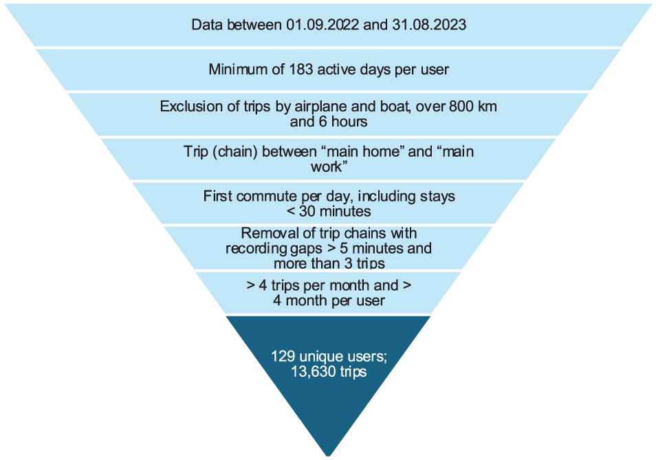
Data filtering.

Figure 2.

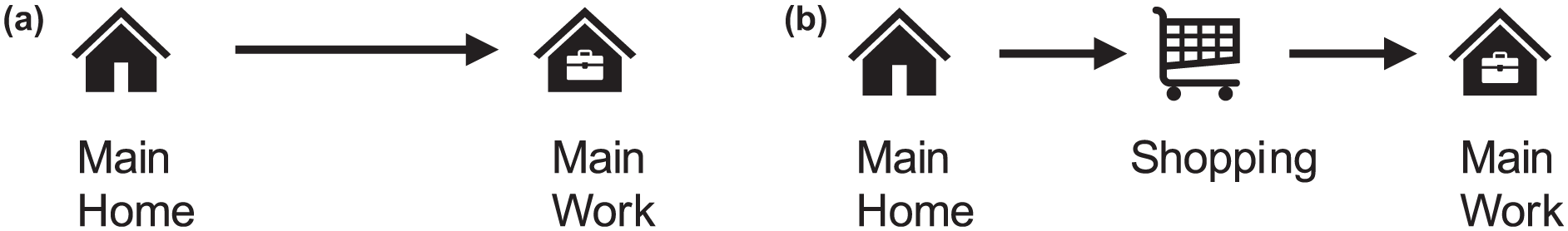
Types of commuting trips: (a) without trip chaining and (b) with trip chaining.

Describing and Modeling Variability: Indicators and Analytical Techniques

This study utilized four distinct methods to assess intraperson modal variability. First, we described the distribution of modal variability using a series of indicators. We then employed a modeling approach comprising beta regressions, a PCA with k-means clustering, and finally, a survival analysis.

Indicators

We chose a larger number of indicators to capture different aspects of commuting variability and provide more robust results. All indicators were calculated on the individual level. The indicators are depicted in Table 2. For the difference in the share of the primary and the alternative main mode (SD) and the normalized HHI, we calculated both the standard version, including all modes, and a simplified version, grouping transportation modes into three mode categories ( 19 ).

Private motorized transportation: This category includes car, motorbike, electric car, carsharing services, and taxi/ride-hailing services;

Public transportation: This category encompasses bus, subway, light rail, regional train, tram, train, and other public transportation modes; and

Active transportation: This category comprises walking, bicycling, kick scooter, electric bicycle, and bike-sharing services.

Table 2.

Indicators

Indicator	Explanation	Formula	Range
Commuter Main Mode Choice Matrix ( 14 )	A matrix representing the distribution of the most used (primary) main mode and second most used (alternative) main mode among commuters	na	na
Total number of unique main modes ( 14 , 19 )	Number of different main modes the participant used to commute between their main home and main workplace	$U = count (unique modes)$	$[1, n]$ where $n$ is the total number of modes
Difference in the share of the primary and alternative main mode ( 19 )	The difference in proportion between the primary main mode and the alternative main mode	$SD = S_{p} - S_{a}$ where $S_{p}$ is the share of the primary main mode and $S_{a}$ is the share of the alternative main mode	$[0, 1] :$ 0 means that the primary and the alternative main mode are used equally, 1 indicates that only one main mode is used
Normalized Herfindahl–Hirschman index (HHI) ( 19 , 24 )	A measure of mode concentration, originally used to describe markets	$HH I_{normalized} = \frac{HHI - \frac{1}{n}}{1 - \frac{1}{n}}$ where $HHI = \sum_{i = 1}^{n} s_{i}^{2}$ and $s_{i}$ represents the share of commuting trips made by mode $i$ as a rate, $n$ is the total number of commuting modes	$[0, 1]$ : 0 means maximum diversity, 1 means maximum concentration
Trip chaining rate (TCR) ( 23 )	The rate of commuting trips that contain intermediate stays	$TCR = \frac{Number of chained trips}{Total trips}$	$[0, 1]$

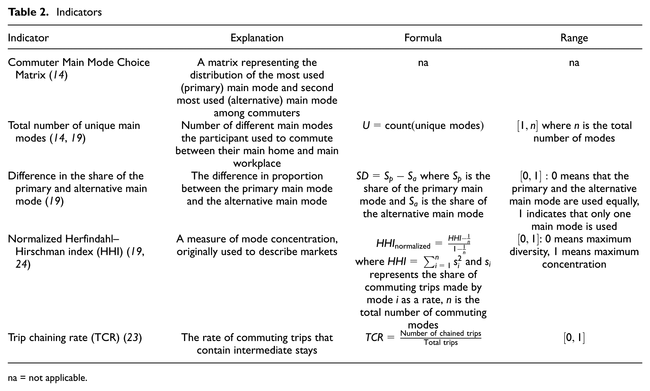
na = not applicable.

Although the nongrouped indicators show variability across all individual modes, the grouped indicators are more effective at showing whether individuals use different types of transportation. An individual who uses bus, tram, light rail, and subway equally for commuting would have high variability across all modes but low variability across mode categories because all modes are public transportation. Therefore, we decided to include both the grouped and nongrouped indicators.

Beta Regression Models

To model the difference in the share of the primary and alternative main mode, the normalized HHI, and the trip chaining rate, we used beta regression models. These models can be used to model proportions, values between 0 and 1 ( 31 ).

Principal Component Analysis and K-Means Clustering

To analyze changes in commuting mode over time, we segmented the data into user-months. For each user-month, we calculated the share of private motorized transportation, public transportation, and active transportation. We then reduced the dimensions using principal components. Since the three values add up to 1, the first two principal components can explain 100% of the variance. We then used the two principle components for k-means clustering to identify commuter modal types.

Survival Analysis

Finally, we utilized survival analysis to describe the stability of the commuter modal types. The survival function was fitted using the Kaplan–Meier method ( 32 ).

Results

Descriptive Statistics

Table 3 illustrates the distribution of socioeconomic variables in the remaining sample. Economic status was estimated using three variables: household income, household size, and the presence of children. This approach was adapted from Nobis and Kuhnimhof ( 33 ) and adjusted for the higher cost of living in the Munich region. As can be observed, certain groups were underrepresented in the dataset, including individuals with mobility impairment or those living in a rural region. These variables were subsequently excluded from the modeling process, given the limited variance observed in the sample. In our GPS-tracking app, we could not distinguish between carpooling and regular driving. Therefore, some car journeys could actually be carpooling journeys. However, carpooling is not very common in Germany, with an average occupancy rate for commutes of 1.1 people ( 34 ). Table 3 also provides an overview of the processed commuting trips in the dataset. The variables were first aggregated at the user level. Compared with average commuting trips in urban regions ( 35 ), our sample showed a high modal share of cycling (35% versus 14%) and a lower car use (17% versus 57%). Given that the participants in the study were recruited through the media and that the study focused on Germany’s 9-Euro-Ticket, the country’s low-fare ticket in 2022, it can be reasonably assumed that individuals with a greater interest in sustainable transportation were more likely to participate.

Table 3.

Data Description

(a) Description of Study Participants

Variable	Percentage	Level
Age	17.1	18–29
	23.3	30–39
	25.6	40–49
	24.0	50–59
	10.1	60–70
Economic status	47.3	(Very) high
	30.3	Middle
	19.7	(Very) low
Gender	53.5	Male
Gender	46.5	Female
Mobility impairment	95.9	No
Mobility impairment	4.1	Yes
Home in rural region	98.4	No
Home in rural region	1.6	Yes
Children	70.2	No
Children	29.8	Yes
Driver’s license	6.3	No
Driver’s license	93.7	Yes

(b) Summary Statistics for Commuting Trips
Variable	Mean	Min.	Max.
Total trips	105.66	28	207
Months recorded	9.53	5	12
Trips/month	10.82	5.60	17.90
Trip duration (min)	31.36	5.74	73.58
Trip distance (km)	11.60	0.61	58.67
Public transport access (modes)	1.83	0	4
Trip chaining (%)	7.55	0.00	53.90
Main: bus	7.65	0.00	97.70
Main: car	17.03	0.00	100.00
Main: bicycle	34.71	0.00	100.00
Main: walk	2.97	0.00	98.89
Main: e-car	2.45	0.00	100.00
Main: motorbike	0.46	0.00	38.61
Main: kick scooter	0.00	0.00	0.50
Main: subway	18.97	0.00	99.26
Main: car sharing	0.02	0.00	1.47
Main: light rail	9.63	0.00	100.00
Main: taxi/uber	0.00	0.00	0.52
Main: regional train	2.56	0.00	97.62
Main: e-bike	1.61	0.00	55.56
Main: tram	1.69	0.00	71.77
Main: bike sharing	0.03	0.00	2.16
Main: train	0.02	0.00	2.17
Main: other	0.19	0.00	22.22

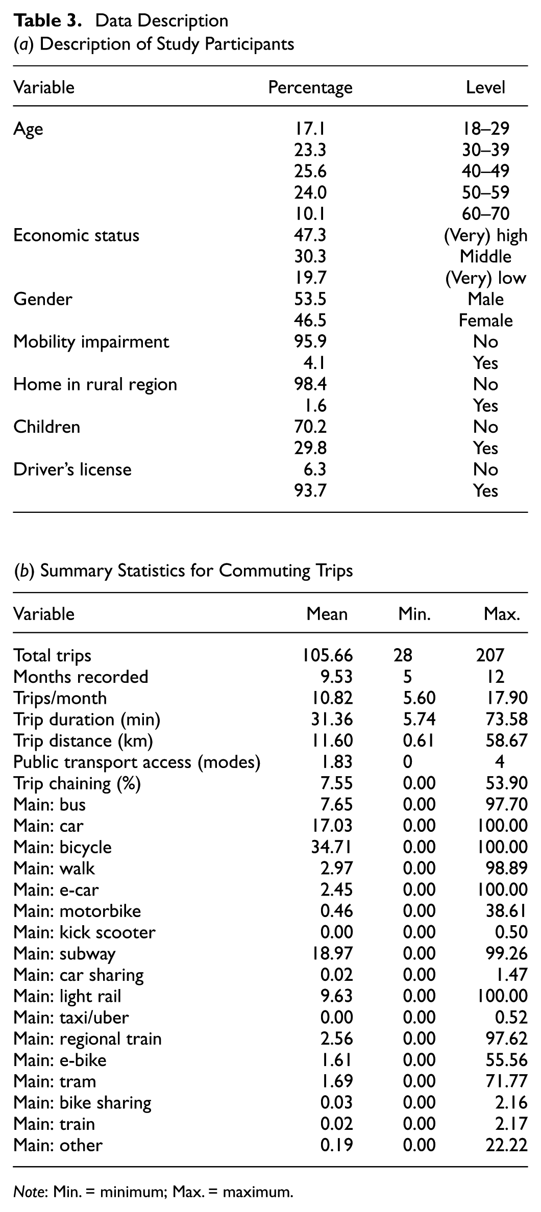
Note: Min. = minimum; Max. = maximum.

Commuter Main Mode Choice Matrix

The commuter main mode choice matrix (Table 4) illustrates which main modes are often used in combination with each other. The most common combinations are among others, bicycle and subway, bicycle and bus, bicycle and car, and car and light rail.

Table 4.

Commuter Main Mode Choice Matrix

Primary	Alternative main modes
Primary	Bicycle	Bus	Car	Carsharing	E-bike	Light rail	Motorbike	Other	Regional train	Subway	Tram	Walk
Bicycle	na	8	6	1	0	3	0	1	0	15	4	7
Bus	4	na	2	0	1	1	0	0	0	1	1	1
Car	6	3	na	1	0	6	2	0	1	2	0	1
E-bike	1	na	0	0	na	1	0	0	0	0	1	0
E-car	0	na	1	0	0	1	0	0	0	0	0	0
Light rail	4	na	4	0	0	na	0	0	1	2	0	0
Regional train	0	na	2	0	0	1	0	0	na	0	0	0
Subway	8	3	7	0	2	2	0	0	0	na	1	0
Tram	1	na	0	0	0	0	0	0	0	0	na	0
Walk	2	na	0	0	0	0	0	0	0	0	0	na

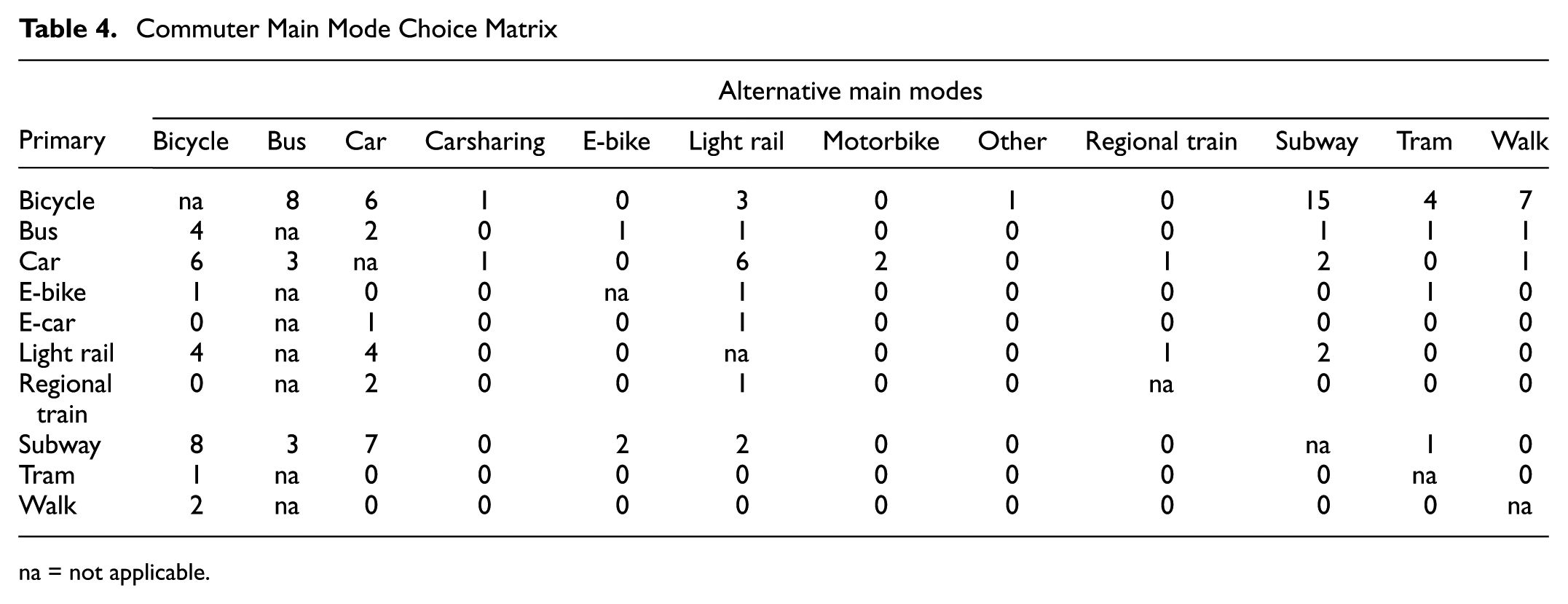
na = not applicable.

Total Number of Unique Main Modes (U)

Figure 3a demonstrates that the distribution is right-skewed, with only six out of 129 study participants relying on only one mode during the observation period. On average, our study participants used three different main modes for their home-to-work trips.

Figure 3.

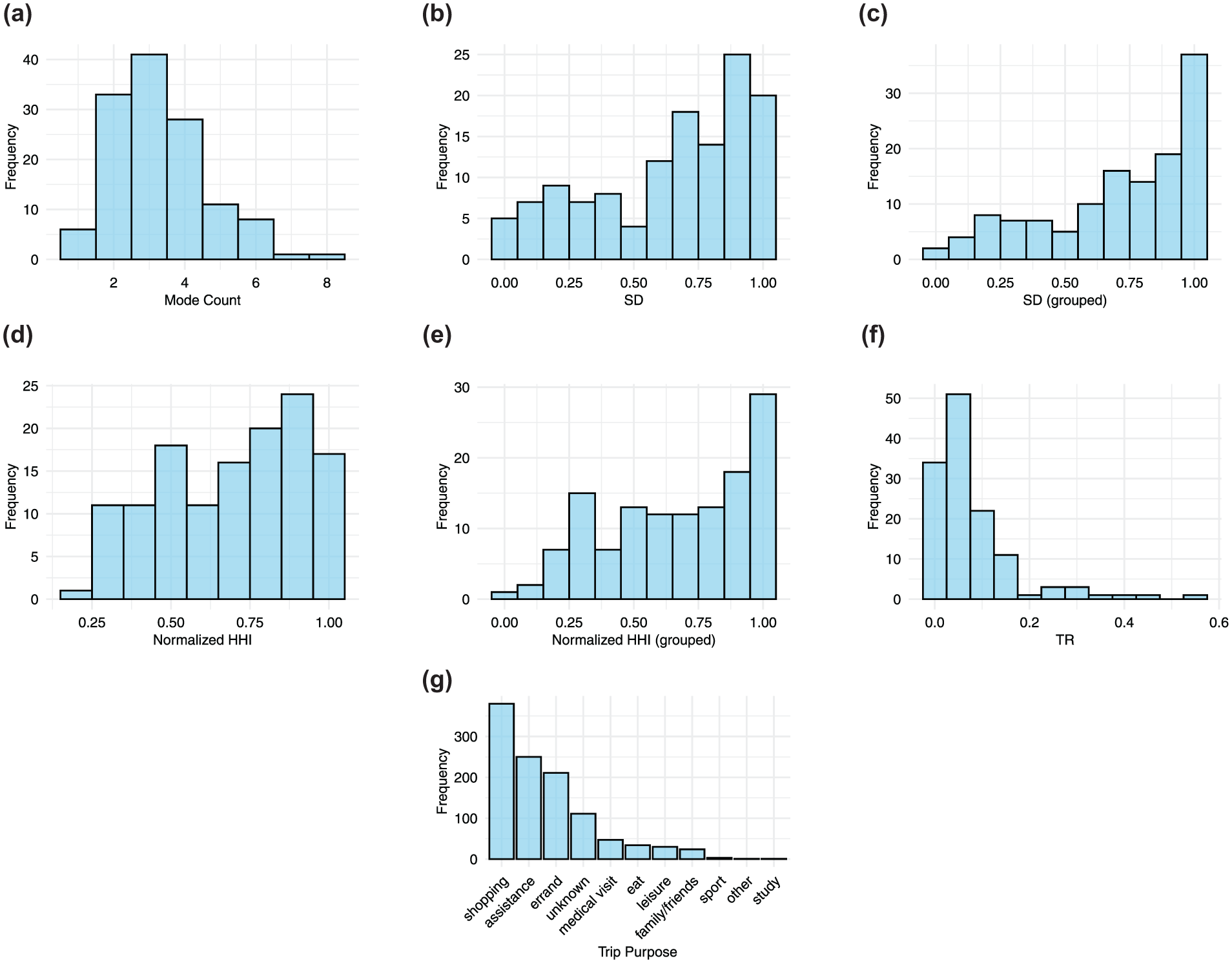
Indicators of modal variability: (a) unique main modes, (b) share difference, (c) share difference (grouped), (d) normalized HHI, (e), normalized HHI (grouped), (f) trip chaining rate, and (g) trip chaining purpose.

Difference in the Share of the Primary and Alternative Main Mode (SD)

Figure 3, b and c , depicts the difference in the share of the primary and alternative main mode. Values close to 1 indicate a higher concentration on one mode, whereas a value of 0 would mean that the primary and alternative main modes are used equally. For all modes, the average value of the indicator was 0.64, for the grouped modes it was 0.7. Both indicators were spread across the entire range in our sample.

Normalized Herfindahl–Hirschman Index

The results for the normalized HHI are shown in Figure 3, d and e . The mean values were 0.69 and 0.66 for the HHI using all modes and the grouped modes, respectively. These mean values were very similar to those found by Heinen and Chatterjee ( 19 ).

Trip Chaining Rate

To further understand the variability of commuting trips, we also analyzed trip chains on the commute to work. Figure 3f displays the percentage of commuter trips that contain trip chains. About 7.9% of commuters never combined their home-to-work trip with other purposes, the average percentage for trip chaining during the commute was 7.5%, this means that 7.5% of all commuting trips included intermediate stays. Figure 3g visualizes the most common purposes between home and work. The most common purpose was shopping, followed by assistance and errands.

Modeling Variability with Beta Regression Models

To identify factors that contribute to the variability of commuting, we fitted beta regression models on three indicators: SD (all modes and grouped), the normalized HHI (all modes and grouped), and trip chaining rate (TCR). We included socioeconomic variables, information on access to various public transportation modes, and possession of a driver’s license as predictors (Table 5).

Table 5.

Results from the Beta Regression Models

Variable	SD	SD (grouped)	Normalized HHI	Normalized HHI (grouped)	TCR
Variable	Coef (SE)	z-value	Coef (SE)	z-value	Coef (SE)	z-value	Coef (SE)	z-value	Coef (SE)	z-value
(Intercept)	0.98 (0.63)	1.56	2.19*** (0.62)	3.52	1.36* (0.56)	2.41	2.08*** (0.62)	3.34	−2.15*** (0.48)	−4.48
Gender: female	0.41. (0.22)	1.85	0.16 (0.22)	0.74	0.41* (0.20)	2.09	0.21 (0.22)	0.95	−0.46** (0.17)	−2.61
Has children	−0.07 (0.26)	−0.26	−0.15 (0.26)	−0.63	0.00 (0.23)	0.01	−0.16 (0.26)	−0.63	0.30 (0.20)	1.50
Driver’s license	−0.39 (0.52)	−0.77	−1.11* (0.50)	−2.23	−0.33 (0.46)	−0.71	−1.18* (0.50)	−2.38	−0.40 (0.38)	−1.05
Access PT modes	−0.13 (0.12)	−1.11	−0.09 (0.12)	−0.76	−0.18. (0.11)	−1.72	−0.08 (0.12)	−0.69	0.02 (0.09)	0.25
Age: 30–39	0.31 (0.37)	0.83	0.16 (0.37)	0.44	0.34 (0.33)	1.04	0.22 (0.37)	0.59	0.27 (0.29)	0.92
Age: 40–49	0.11 (0.37)	0.29	0.17 (0.37)	0.47	−0.00 (0.33)	−0.00	0.13 (0.37)	0.35	0.16 (0.29)	0.56
Age: 50–59	0.42 (0.38)	1.10	0.47 (0.38)	1.23	0.50 (0.34)	1.46	0.56 (0.38)	1.46	−0.24 (0.30)	−0.78
Age: 60–70	−0.07 (0.46)	−0.15	−0.18 (0.46)	−0.39	−0.17 (0.40)	−0.42	−0.19 (0.46)	−0.41	0.00 (0.36)	0.01
Economic status: (very) low	−0.18 (0.31)	−0.60	−0.31 (0.31)	−1.02	−0.16 (0.27)	−0.60	−0.27 (0.31)	−0.88	0.01 (0.24)	0.03
Economic status: middle	−0.32 (0.25)	−1.30	−0.53* (0.25)	−2.13	−0.43. (0.22)	−1.94	−0.55* (0.25)	−2.19	0.14 (0.19)	0.74
Log-likelihood	37.45	na	92.19	na	49.48	na	76.59	na	211.60	na
Pseudo R²	0.06	na	0.08	na	0.08	na	0.08	na	0.08	na
N	122	na	122	na	122	na	122	na	122	na
Phi	1.54*** (0.17)	9.07	1.44*** (0.17)	8.51	2.63*** (0.31)	8.40	1.45*** (0.17)	8.72	8.52*** (1.24)	6.87

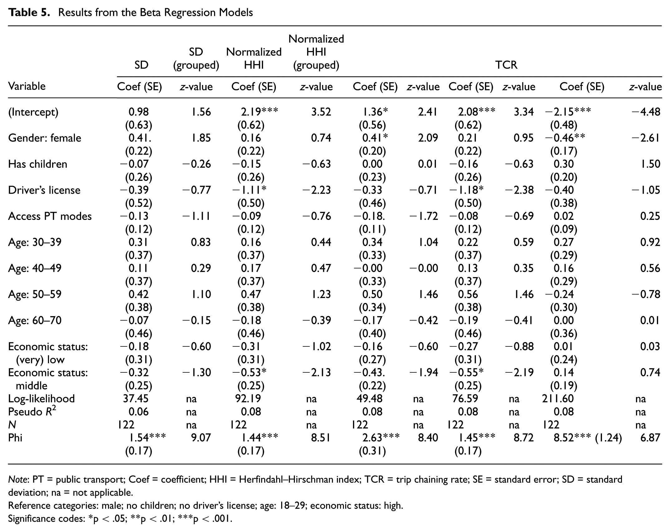
Note: PT = public transport; Coef = coefficient; HHI = Herfindahl–Hirschman index; TCR = trip chaining rate; SE = standard error; SD = standard deviation; na = not applicable.

Reference categories: male; no children; no driver’s license; age: 18–29; economic status: high.

Significance codes: *p < .05; **p < .01; ***p < .001.

For the SD and the normalized HHI (grouped), we found that being female was negatively related to modal variability. It was also negatively associated with TCR. Having a driver’s license was positively associated with higher variability for the grouped SD and the grouped HHI. For the same indicators, individuals with a middle economic status were associated with higher variability compared with individuals with a (very) high economic status. Overall, modal flexibility seemed to be barely deterministic, as the pseudo R-squared values of our models were relatively low. Other studies have also found difficulties in modeling modal variability, with pseudo R-squared values below 0.1 ( 11 ).

Commuting Variability over Time

To classify commuter modal types and track changes over time, we continued with the classification of modes into private motorized transportation, public transportation, and active transportation. We calculated the share of each mode category per user-month and employed PCA. In the next step, we used both the elbow and the silhouette method to determine the optimal number of clusters for k-means, as depicted in Figure 4.

Figure 4.

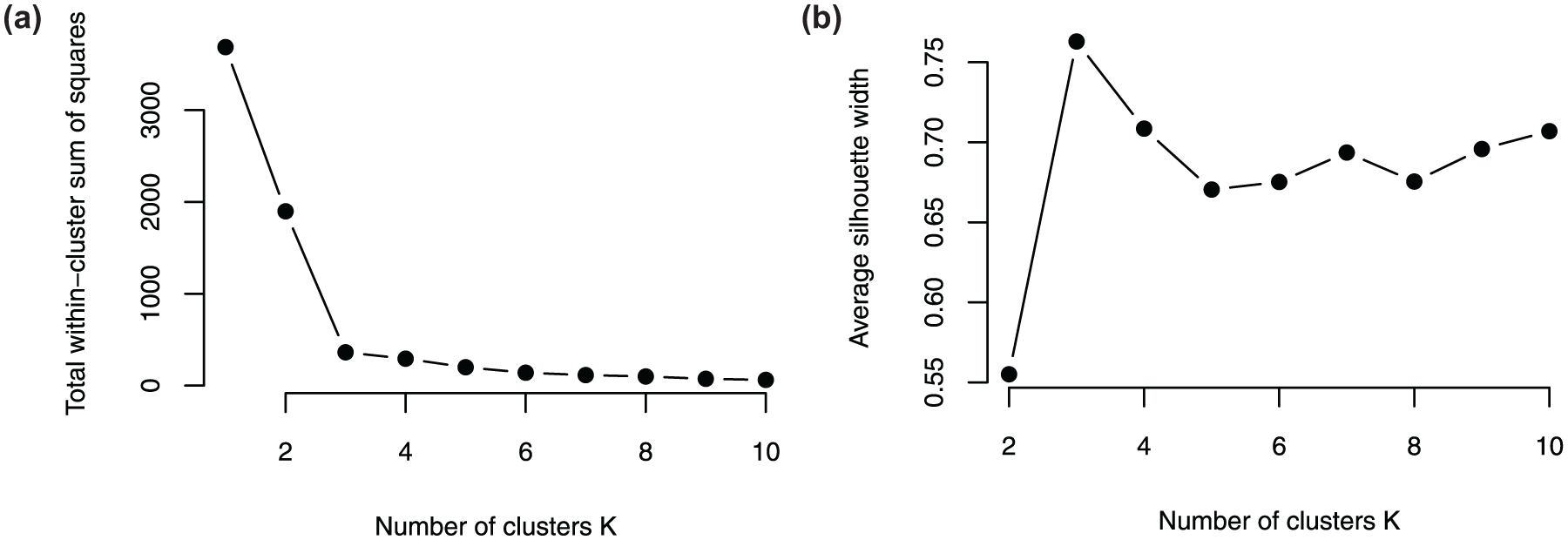
Determining the number of clusters: (a) elbow method and (b) silhouette method.

K-means clustering could explain over 90% of the variance, using three clusters. Interpreting the cluster centers and the loadings of the principal components, Cluster 1 (N = 517) corresponded to predominantly active transportation users, Cluster 2 (N = 246) to predominantly private transportation users, and Cluster 3 (N = 467) to predominantly public transportation users (see Figure 5).

Figure 5.

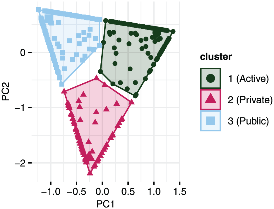
K-means clustering.

The shape of the data points on the two principal components in space can be explained by the constraints of the variables: all mode category proportions range between 0 and 1, and the three proportions add up to 1. The data points at the corners of the triangle represent user-months dominated by a single mode category: the bottom corner indicates exclusively private motorized transportation users, the left corner indicates exclusively public transportation users, and the right corner indicates exclusively active transportation users. The data points along the edges represent user-months where two out of the three mode categories were used.

Descriptive statistics for the commuter modal types are shown in Figure 6 and Table 6. Since cluster memberships were estimated monthly, users who stayed in the cluster longer had more weight in the cluster statistics. The analysis of the commuting clusters revealed notable differences in trip characteristics and demographic profiles. Cluster 1 (active) had the shortest trip duration (22.5 min) and distance (5.4 km). In contrast, Cluster 2 (private) had the longest average trip distance (20.0 km), reflecting longer commutes associated with private vehicle use. Cluster 3 (public) had the longest commute duration, with an average trip duration of 40.3 min. Demographically, Cluster 1 was characterized by a lower percentage of women (41.2%) and fewer individuals with a driver’s license (94.2%), whereas Cluster 2 had the highest percentage of individuals with a (very) high economic status (56.5%).

Figure 6.

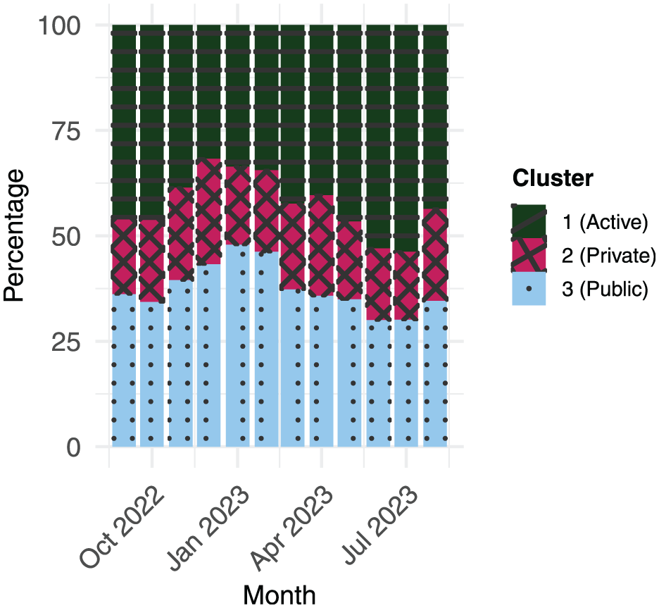
Commuter modal types: percentage of each cluster by month.

Table 6.

Descriptive Statistics of the Commuter Modal Types

Variable	Cluster 1 (active)	Cluster 2 (private)	Cluster 3 (public)
Gender: female (%)	41.2	42.3	52.5
Children (%)	34.7	30.5	25.9
Driving license (%)	94.2	100	88.6
Number of different public transport modes in 5 minute walking distance	2.1	1.4	1.8
Home in rural region (%)	0.0	4.1	1.7
Mobility impairment (%)	3.4	9.3	3.9
Trip duration (min)	22.5	30.1	40.3
Trip distance (km)	5.4	20.0	14.0
Age: 18–29 (%)	18.2	5.2	18.4
Age: 30–39 (%)	26.5	27.2	18.0
Age: 40–49 (%)	32.1	33.5	19.5
Age: 50–59(%)	16.4	23.5	30.0
Age: 60–70 (%)	6.7	11.4	14.1
Economic status: (very) high (%)	47.9	56.5	43.0
Economic status: middle (%)	27.6	26.4	32.3
Economic status: (very) low (%)	18.9	13.8	18.8

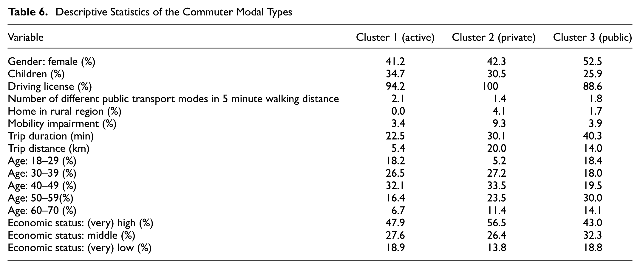
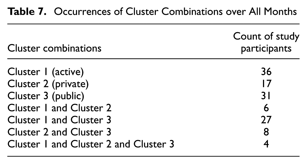
Table 7 demonstrates that commuter modal types are not necessarily stable over time, with a significant proportion of individuals changing cluster membership even within the multimonth study duration. The percentage of each cluster per month is visualized in Figure 6. Notably, the share of Cluster 1 (active) decreased during the winter months, whereas the share of Cluster 3 (public) increased. It is important to note that the sample size for August was small, so the shares for that month may not be representative. In our sample, 65.1% of individuals stayed in the same commuting cluster for the entire observation period, 31.8% belonged to two clusters, and 3.1% to all clusters. Although staying within a cluster was the most common case, especially between Cluster 1 (active) and Cluster 3 (public), membership seemed to be more flexible.

Table 7.

Occurrences of Cluster Combinations over All Months

Cluster combinations	Count of study participants
Cluster 1 (active)	36
Cluster 2 (private)	17
Cluster 3 (public)	31
Cluster 1 and Cluster 2	6
Cluster 1 and Cluster 3	27
Cluster 2 and Cluster 3	8
Cluster 1 and Cluster 2 and Cluster 3	4

Furthermore, we used survival analysis to describe the stability of the commuter modal type. The event used in the survival analysis was leaving the cluster in which the individual started. We only considered the first cluster change. Individuals who never changed their commuter modal type during the observation period were considered censored in our survival analysis.

Figure 7 presents the survival curve. At the 5-month mark, 71.1% of the subjects were estimated to have remained in their original cluster, with a 95% confidence interval (CI) ranging from 63.6% to 79.4%. At the 10-month mark, 58.9% of the subjects were estimated to have stayed in their starting cluster, with a 95% CI ranging from 48.8% to 71.0%. Although these values suggest a certain “stickiness” of the commuter modal type, they also highlighted that a significant share of commuters changed their main transportation mode for commuting within a longer period.

Figure 7.

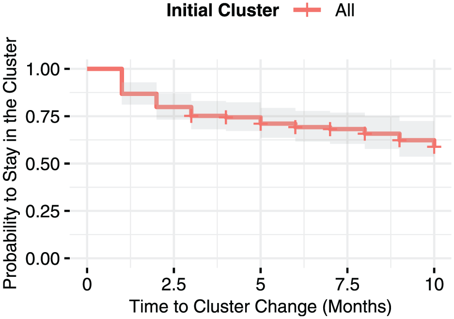
Survival analysis (all clusters).

In Figure 8, separate survival functions were estimated for each cluster. Because cluster transitions did not occur each month for each cluster, the survival estimates for months without transitions did not change. At the 5-month mark, 59.9% of subjects in initial Cluster 1 (Active) were estimated to have remained, with a 95% CI ranging from 48.7% to 73.7%. For Cluster 2 (Private), the probability was 86.4% (95% CI: 73.2% to 100%), and for Cluster 3 (Public), the probability was 78.2% (95% CI: 67.1% to 91.2%). The data suggested that individuals who used predominantly private motorized transportation were less likely to change their commuter modal type within a 5-month period compared with other groups. However, standard errors were large owing to the limited sample size.

Figure 8.

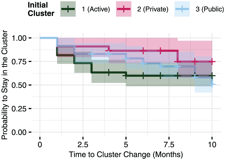
Survival analysis by cluster membership.

Figure 9 presents the probability of transitioning between commuter modal clusters based on the previous month’s cluster membership. This analysis only included user-months in which at least five commuting trips were recorded in the previous month. To account for the small sample size, 95% Wilson CIs were computed. As shown in the figure, there was limited evidence that seasonality significantly influenced commuter modal type. Although more individuals appeared to transition from active to public transportation in December and from public transportation to active in June, the confidence intervals were wide (11% to 36% and 11% to 39%, respectively), indicating substantial uncertainty in these estimates.

Figure 9.

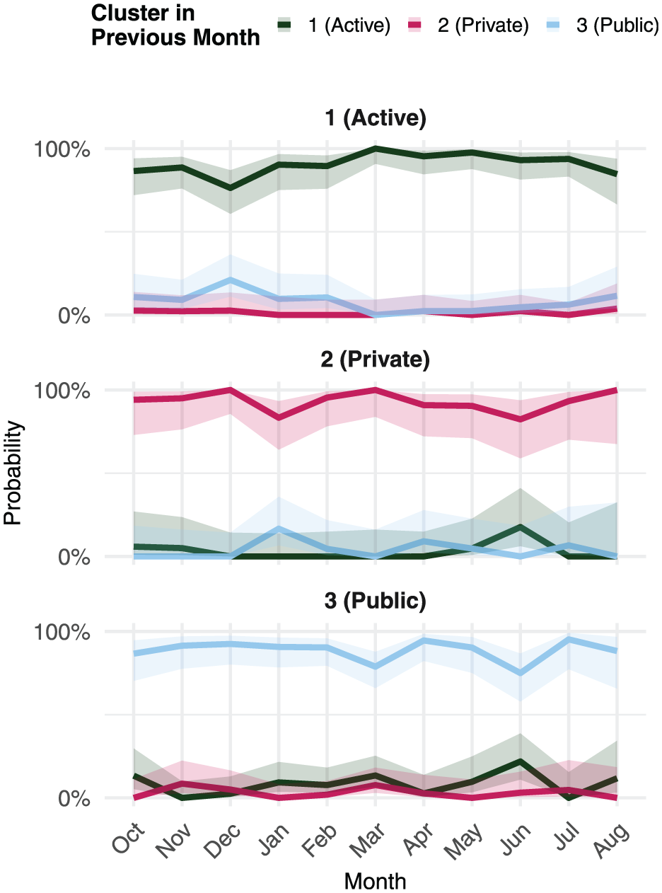
Transition probabilities between commuter modal clusters.

Figure 10 provides further insights by distinguishing between temporary and permanent changes in commuter modal type. To reduce the influence of random fluctuations in the first month, the start cluster was determined based on the most frequent cluster in the first three recorded months. Among users who started in the active transportation cluster, 64% remained in the same cluster for all recorded months, 13% permanently switched to a different cluster, and 20% transitioned to another cluster before returning to their original one. For users who initially belonged to the private transportation cluster, the respective figures were 77%, 14%, and 9%, whereas for the public transportation cluster, they were 61%, 16%, and 20%. These results suggest that private transportation exhibited higher “stickiness,” meaning individuals in this cluster were less likely to switch modal types. In contrast, active and public transportation clusters showed greater fluctuations, indicating more dynamic commuting patterns. Temporary changes in commuter modal types may be influenced by disruptive factors affecting the usual mode, such as temporary public transportation closures or adverse weather conditions. Additionally, since commuter modal type is a discrete classification, individuals with multimodal travel patterns may appear to have switched modes even when their overall behavior remains largely unchanged. For example, a commuter using public transportation for 60% of trips and active transportation for 40% in one month, then shifting to a split of 40/60 in the following month, would be classified as having changed modal type despite only small changes in actual travel behavior.

Figure 10.

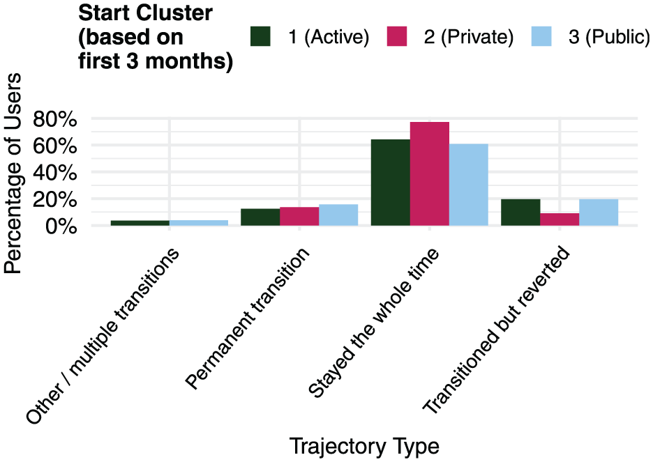
Trajectory types of commuter modal changes.

Discussion

Using different indicators, we observed variability in commuting mode choice in our dataset. Moreover, our data suggested variability in the variability. We found that being female was negatively associated with modal variability as measured by the share difference and the normalized HHI. This is in line with other studies, finding systematic gendered differences in commuting styles ( 36 ). However, the variable was not significant for the grouped version of the indicators. This suggests that men tend to be more variable in their modes of transportation, but not in the broader mode categories (active transportation, private motorized transportation, public transportation). Having a driver’s license was negatively associated with the grouped versions of the indicators, indicating higher modal variability. This finding is very intuitive, as individuals without a driving license cannot use private motorized transportation as a driver, which limits the use of this mode category. Finally, individuals with a middle economic status tended to have a higher variability in commuting modes compared with individuals with a (very) high economic status. This finding could be explained by individuals with a higher economic status being able to afford their preferred mode and stay with it; individuals with lower economic status may stay with fewer modes because they do not have many options, for example, because they are transit captives ( 37 ). Overall, the models had a low model fit, suggesting that modal variability has a low deterministic nature. This could be explained by unobserved variables, such as psychological scales of openness or curiosity. For future analyses, hurdle models could be used to distinguish between individuals who tend to be monomodal and those who show high variability in regard to their mode of transportation for commuting trips. Analyzing the commuter modal type over time using clusters, we saw that whereas the majority of commuters remained in their cluster, a significant proportion of 32% changed cluster membership. In particular, we observed individuals switching from active transportation to public transportation in the colder months, suggesting the influence of weather. Membership in the cluster dominated by private motorized transportation seemed to be more stable over time. This could be explained by a strong preference for car use or a lack of (attractive) alternatives. The latter explanation is supported by individuals in this cluster having higher home-to-work travel distances and fewer public transportation options near their homes. Because of data availability, our unit of analysis in the survival analysis was the user-month, so that we could identify coarser changes in commuting mode over months rather than fluctuations within a week.

There were several limitations to our analysis. We had a relatively small sample size, an overrepresentation of bicycle commuters, and an underrepresentation of car commuters. Since active mode commuters are more likely to change their commuting mode over time, our results for modal variability may be biased upward. Given the exploratory nature of our study and the constraints of a small sample size, our primary goal was to analyze patterns within this specific population rather than generalizing across all commuting behavior. Therefore, the study’s findings are limited to the participants sampled and should be interpreted accordingly. Finally, we did not include working from home as an alternative in our analysis. If individuals have the option of working from home, this could reduce their modal variability. If their preferred mode becomes unattractive owing to traffic congestion or rain, for example, they might choose to stay home.

Conclusion

In this article, we analyzed the modal variability of home-to-work trips among 129 individuals who recorded, on average, 10 months of GPS data using a smartphone app. Our analysis of transportation mode choices revealed that few individuals were monomodal in their commuting trips; the majority used three or more different main modes at least once during the observation period. The commuter main mode choice matrix indicated that the most common combinations were bicycle and subway, bicycle and bus, bicycle and car, and car and light rail, highlighting the role of active mobility as a substitute for other modes. We observed a wide range in the continuous indicators, difference in the share of the primary and alternative modes (SD) and HHI, demonstrating that our sample included both flexible commuters and individuals who tend to concentrate on a few modes rather than displaying diverse transportation options for home-to-work trips. Further analysis showed that being female was negatively related to modal variability, whereas having a driver’s license was positively associated with higher variability. Additionally, individuals with middle economic status exhibited greater variability in their mode choices compared with those with very high economic status. However, the low R-squared values indicated that the independent variables in the models did not fully account for modal variability.

In conclusion, although it is well-established that “human trajectories show a high degree of temporal and spatial regularity” ( 38 ), arguably driven by strong habitual patterns such as commuting, our findings provide further insight into this behavior. Specifically, we found that 65% of the sample maintained consistent travel modes for commuting over a 10-month period. However, using advances in GPS-based mode detection, we also revealed that around one-third of commuters demonstrated significant variability in their transportation modes over time, changing their commuter modal type at least once. These findings have important implications for the development of innovative CDM policy instruments aimed at mitigating the negative externalities of commuter mobility, such as tradable credit schemes ( 39 ) and mobility-based charging ( 40 ). Future research should focus especially on the variability shown by car users and identify events/policies that make changes in commuter modal type more likely.

Footnotes

Acknowledgements

The authors would like to thank the TUM Think Tank at the Munich School of Politics and Public Policy for its support. We thank Santiago Álvarez-Ossorio Martínez for his algorithm for identifying the main work and home locations and for his useful comments. GPT-4 assisted in debugging the R code, creating LaTeX tables, and making language edits.

Author Contributions

The authors confirm contribution to the paper as follows: study conception and design: I. Waldorf, A. Loder, J. Müller; data collection: A. Loder; analysis and interpretation of results: I. Waldorf, A. Loder, J. Müller, V. Dahmen; draft manuscript preparation: I. Waldorf, J. Müller, A. Loder, V. Dahmen, K. Bogenberger. All authors reviewed the results and approved the final version of the manuscript.

Declaration of Conflicting Interests

The authors declared no potential conflicts of interest with respect to the research, authorship, and/or publication of this article.

Funding

The authors disclosed receipt of the following financial support for the research, authorship, and/or publication of this article: I. Waldorf and J. Müller received funding from the MINGA project (grant no. 45AOV1001A-N). A. Loder received funding from the Bavarian State Ministry of Science and the Arts in the framework of the Bavarian Research Institute for Digital Transformation (bidt) Graduate Center for Postdocs. Further, A. Loder received support from the German Research Foundation (grant no. 525732760) for the project READAPT. V. Dahmen received funding from the TUM Georg Nemetschek Institute Artificial Intelligence for the Built World.

ORCID iDs

Isabella Waldorf

Allister Loder

Johannes Müller

Victoria Dahmen

Klaus Bogenberger

References

Umweltbundesamt. Emissionen des Verkehrs. 2024. https://www.umweltbundesamt.de/daten/verkehr/emissionen-des-verkehrs#verkehr-belastet-luft-und-klima-minderungsziele-der-bundesregierung. Accessed July 10, 2024.

United States Environmental Protection Agency. Carbon Pollution from Transportation. 2024. https://www.epa.gov/transportation-air-pollution-and-climate-change/carbon-pollution-transportation. Accessed July 10, 2024.

Verkehrswende

Pendlerverkehr. Technical Report. 2022. https://www.agora-verkehrswende.de/fileadmin/Projekte/2022/Pendlerverkehr/77_Pendlerverkehr.pdf. Accessed July 10, 2024.

Wang

Geng

May

A. D.

Zhou

The Impact of Traffic Demand Management Policy Mix on Commuter Travel Choices. Transport Policy, Vol. 117, 2022, pp. 74–87.

Farahmand

Z. H.

Gkiotsalitis

Geurs

K. T.

Mobility-as-a-Service as a Transport Demand Management Tool: A Case Study Among Employees in the Netherlands. Case Studies on Transport Policy, Vol. 9, No. 4, 2021, pp. 1615–1629.

Ribeiro

P. J.

Fonseca

Students’ Home-University Commuting Patterns: A Shift Towards More Sustainable Modes of Transport. Case Studies on Transport Policy, Vol. 10, No. 2, 2022, pp. 954–964.

Whillans

Sherlock

Roberts

O’Flaherty

Gavin

Dykstra

Daly

Nudging the Commute: Using Behaviorally Informed Interventions to Promote Sustainable Transportation. Behavioral Science & Policy, Vol. 7, No. 2, 2021, pp. 27–49.

Aarts

H. H.

Verplanken

van Knippenberg

Predicting Behavior from Actions in the Past: Repeated Decision Making or a Matter of Habit?

Journal of Applied Social Psychology, Vol. 28, 1998, pp. 1355–1374. https://api.semanticscholar.org/CorpusID:14980108.

Heinen

Ogilvie

Variability in Baseline Travel Behaviour as a Predictor of Changes in Commuting by Active Travel, Car and Public Transport: A Natural Experimental Study. Journal of Transport & Health, Vol. 3, No. 1, 2016, pp. 77–85. https://doi.org/10.1016/j.jth.2015.11.002.

10.

Pas

E. I.

Koppelman

F. S.

An Examination of the Determinants of Day-to-Day Variability in Individuals’ Urban Travel Behavior. Transportation, Vol. 13, No. 2, 1986, pp. 183–200. https://doi.org/10.1007/BF00165547.

11.

Chatterjee

Clark

Bartle

Commute Mode Choice Dynamics: Accounting for Day-to-Day Variability in Longer Term Change. European Journal of Transport and Infrastructure Research, Vol. 16, No. 4, 2016, pp. 713–734. https://doi.org/10.18757/EJTIR.2016.16.4.3167.

12.

Montini

Rieser-Schüssler

Horni

Axhausen

K. W.

Trip Purpose Identification from GPS Tracks. Transportation Research Record: Journal of the Transportation Research Board, 2014. 2405: 16–23.

13.

Hong

Martin

Xin

Bucher

Reck

D. J.

Axhausen

K. W.

Raubal

Conserved Quantities in Human Mobility: From Locations to Trips. Transportation Research Part C: Emerging Technologies, Vol. 146, 2023, p. 103979. https://doi.org/10.1016/j.trc.2022.103979.

14.

Arifin

Z. N.

Axhausen

K. W.

Investigating Commute Mode and Route Choice Variability in Jakarta Using Multi-Day GPS Data. Arbeitsberichte Verkehrs- und Raumplanung, Vol. 668, 2011. https://doi.org/10.3929/ETHZ-A-006686135.

15.

Cherchi

Cirillo

Understanding Variability, Habit and the Effect of Long Period Activity Plan in Modal Choices: A Day to Day, Week to Week Analysis on Panel Data. Transportation, Vol. 41, No. 6, 2014, pp. 1245–1262. https://doi.org/10.1007/s11116-014-9549-y.

16.

Chowdhury

La Paix

Geurs

Inter- and Intrapersonal Variation in Destination Choice. European Journal of Transport and Infrastructure Research, Vol. 20, No. 4, 2020, pp. 194–213. https://doi.org/10.18757/ejtir.2020.20.4.3951.

17.

Crawford

Segmenting Travellers Based on Day-to-Day Variability in Work-Related Travel Behaviour. Journal of Transport Geography, Vol. 86, 2020, p. 102765. https://doi.org/10.1016/j.jtrangeo.2020.102765.

18.

Hatcher

S. G.

Mahmassani

H. S.

Daily Variability of Route and Trip Scheduling Decisions for the Evening Commute. Transportation Research Record: Journal of the Transportation Research Board, 1992. 1357: 72–81.

19.

Heinen

Chatterjee

The Same Mode Again? An Exploration of Mode Choice Variability in Great Britain Using the National Travel Survey. Transportation Research Part A: Policy and Practice, Vol. 78, 2015, pp. 266–282. https://doi.org/10.1016/j.tra.2015.05.015.

20.

Raux

T.-Y.

Cornelis

Variability in Daily Activity-Travel Patterns: The Case of a One-Week Travel Diary. European Transport Research Review, Vol. 8, No. 4, 2016, pp. 1–14. https://doi.org/10.1007/s12544-016-0213-9.

21.

Schlich

Measurement Issues in Identifying Variability in Travel Behaviour. Proc., 1st Swiss Transport Research Conference (STRC 2001), Monte Verità, Ascona, Switzerland, March 1–3, 2001. https://doi.org/10.3929/ETHZ-A-004240075.

22.

Shen

Kwan

M.-P.

Chai

Investigating Commuting Flexibility with GPS Data and 3D Geovisualization: A Case Study of Beijing, China. Journal of Transport Geography, Vol. 32, 2013, pp. 1–11. https://doi.org/10.1016/j.jtrangeo.2013.07.007.

23.

Streit

Allier

C.-E.

Weiss

Chlond

Vortisch

Changes in Variability and Flexibility of Individual Travel in Germany. Transportation Research Record: Journal of the Transportation Research Board, 2015. 2496: 10–19. https://doi.org/10.3141/2496-02.

24.

Susilo

Y. O.

Axhausen

K. W.

Repetitions in Individual Daily Activity–Travel–Location Patterns: A Study Using the Herfindahl–Hirschman Index. Transportation, Vol. 41, 2014, pp. 995–1011.

25.

Tarigan

Fujii

Kitamura

Intrapersonal Variability in Leisure Activity-Travel Patterns: The Case of One-Worker and Two-Worker Households. Transportation Letters, Vol. 4, No. 1, 2012, pp. 1–13. https://doi.org/10.3328/TL.2012.04.01.1-13.

26.

Costa

M. A.

Marra

A. D.

Corman

Public Transport Commuting Analytics: A Longitudinal Study Based on GPS Tracking and Unsupervised Learning. Data Science for Transportation, Vol. 5, No. 3, 2023, p. 15. https://doi.org/10.1007/s42421-023-00077-8.

27.

Loder

Cantner

Adenaw

Nachtigall

Ziegler

Gotzler

Siewert

M. B.

, et al. Observing Germany’s Nationwide Public Transport Fare Policy Experiment “9-Euro-Ticket”– Empirical Findings from a Panel Study. Case Studies on Transport Policy, Vol. 15, 2024, p. 101148. https://doi.org/10.1016/j.cstp.2024.101148.

28.

Loder

Cantner

Dahmen

Bogenberger

The Mobilität.Leben Study: A Year-Long Mobility-Tracking Panel. https://doi.org/10.48550/ARXIV.2308.04973.

29.

Dahmen

Álvarez-Ossorio Martínez

Loder

Bogenberger

Making Large Scale Semi-Passive GPS Travel Diaries Valuable: A Quality Enhancement Method. Presented at 103rd Annual Meeting of the Transportation Research Board, Washington, D.C., 2024.

30.

McGuckin

Murakami

Highlights of the 2001 National Household Travel Survey: Trip Chaining. Technical Report. U.S. Department of Transportation, Federal Highway Administration, 2003. https://nhts.ornl.gov/assets/2001/download/TripChaining.pdf.

31.

Ferrari

Cribari-Neto

Beta Regression for Modelling Rates and Proportions. Journal of Applied Statistics, Vol. 31, No. 7, 2004, pp. 799–815.

32.

Bland

J. M.

Altman

D. G.

Survival Probabilities (the Kaplan-Meier Method). BMJ, Vol. 317, No. 7172, 1998, pp. 1572–1580.

33.

Nobis

Kuhnimhof

Mobilität in Deutschland- MiD: Ergebnisbericht. Studie von infas, DLR, IVT und infas 360 im Auftrag des Bundesministers für Verkehr und digitale Infrastruktur (FE-Nr. 70.904/15). Bonn, Berlin, 2018. http://www.mobilitaet-in-deutschland.de

34.

Umweltbundesamt. Fahrgemeinschaften verringern die Kosten und den CO2-Ausstoß, 2024. https://www.umweltbundesamt.de/umwelttipps-fuer-den-alltag/mobilitaet/fahrgemeinschaften. Accessed March 21, 2025.

35.

MIT. Mobilität in Tabellen 2017. Technical Report. Bundesministerium für Verkehr und digitale Infrastruktur (BMVI), 2017. http://www.mobilitaet-in-deutschland.de/MiT2017.html.

36.

Næss

Gender Differences in the Influences of Urban Structure on Daily Travel. In Gendered Mobilities ( Uteng

T. P.

Cresswell

, eds.), Routledge, London, 2016, pp. 173–192.

37.

Beimborn

E. A.

Greenwald

M. J.

Jin

Accessibility, Connectivity, and Captivity: Impacts on Transit Choice. Transportation Research Record: Journal of the Transportation Research Board, 2003. 1835: 1–9.

38.

González

M. C.

Hidalgo

C. A.

Barabási

A.-L.

Understanding Individual Human Mobility Patterns. Nature, Vol. 453, 2008, pp. 779–782. https://doi.org/10.1038/nature06958.

39.

Blum

Hamm

Loder

Bogenberger

Conceptualizing an Individual Full-Trip Tradable Credit Scheme for Multi-Modal Demand and Supply Management: The MobilityCoin System. Frontiers in Future Transportation, Vol. 3, 2022, p. 914496. https://doi.org/10.3389/ffutr.2022.914496; https://www.frontiersin.org/articles/10.3389/ffutr.2022.914496/full.

40.

Bliemer

M. C.

Loder

Zheng

A Novel Mobility Consumption Theory for Road User Charging. Transportation Research Part B: Methodological, Vol. 189, 2024, p. 102998. https://doi.org/10.1016/j.trb.2024.102998; https://linkinghub.elsevier.com/retrieve/pii/S019126152400122X.

Potential for Commuting Demand Management: Analysis of Day-to-Day Modal Variability Based on a 1-Year GPS-Tracking Dataset

Abstract

Keywords

Data and Methodology

Study Design: Mobilität.Leben

Data Filtering

Describing and Modeling Variability: Indicators and Analytical Techniques

Indicators

Beta Regression Models

Principal Component Analysis and K-Means Clustering

Survival Analysis

Results

Descriptive Statistics

Commuter Main Mode Choice Matrix

Total Number of Unique Main Modes (U)

Difference in the Share of the Primary and Alternative Main Mode (SD)

Normalized Herfindahl–Hirschman Index

Trip Chaining Rate

Modeling Variability with Beta Regression Models

Commuting Variability over Time

Discussion

Conclusion

Footnotes

Acknowledgements

Author Contributions

Declaration of Conflicting Interests

Funding

ORCID iDs

References