Sage Journals: Discover world-class research

Abstract

The International Roughness Index is used to measure the road roughness in pavements, as pavement roughness deteriorates over time. Despite many attempts by researchers to predict roughness in concrete pavements, there are limitations, such as small sample size, modeling approach, or lack of robustness in the model. This study presents a novel machine-learning approach incorporating domain knowledge to predict roughness, using a dataset obtained from the Long-Term Pavement Performance database. Physics informed neural networks (PINNs) are popular physics-driven machine-learning approaches that have been receiving widespread attention in the field of civil engineering. PINNs work similarly to neural networks but are augmented with the incorporation of physics-based constraints and governing equations, enabling them to assimilate domain knowledge and leverage physical principles while making predictions or solving problems. In this study, the popular Mechanistic-Empirical Pavement Design Guide roughness prediction model is used along with the optimized neural networks to calculate the physics-based loss function. The Optuna framework is used to tune the hyperparameters within the neural network architecture. The final configuration, optimized and trained in the model, has three hidden layers with, respectively, 27, 67, and 80 neurons. The tuned model has performed well for the testing dataset, with a mean absolute error of 0.134 and a coefficient of determination of 0.90. A sensitivity analysis was also conducted and is presented to understand the influence of the variation of each variable.

Keywords

machine learning (artificial intelligence)neural networks pavements pavement condition evaluation pavement surface properties and roughness

Concrete pavements play a crucial role in modern transportation infrastructure, offering a strong and long-lasting surface for vehicles to travel on. Jointed plain concrete pavements (JPCPs) are widely used forms of concrete pavement with dowels and tie bars and without reinforcement ( 1 ). The initial cost and easy construction practice with high durability give JPCPs an advantage over other types of concrete pavement ( 2 ). However, these pavements can suffer from various forms of damage over time, which can affect ride quality, increase maintenance costs, and shorten their lifespan ( 3 ). It is always a challenge for engineers to maintain and repair concrete pavements to ensure their continued serviceability. The basic requirement to devise effective maintenance strategies is to have a reliable pavement performance model ( 4 ).

Performance metrics, such as the Pavement Condition Index, Pavement Serviceability Index, and Roughness Index, have been extensively utilized to evaluate the functional condition of pavements ( 5 ). Of these, the International Roughness Index (IRI) is an important measure of the ride quality and smoothness of a road surface. It is widely used in pavement maintenance planning as a way to assess the condition of a road and prioritize maintenance and repair activities. There are many parameters that will lead to the progression of roughness over time in concrete pavements. Although there are many studies on the prediction of roughness in asphalt pavements ( 6 ), few researchers have attempted to predict the roughness in concrete pavements ( 7 ). Most of the existing models were developed using traditional approaches for developing roughness prediction. The Mechanistic-Empirical Pavement Design Guide (MEPDG) IRI model for JPCPs is still widely used to predict roughness ( 8 ).

There are also a few studies that have proved that prediction models developed using regression method have not always yielded accurate results ( 9 , 10 ). The deployment of machine learning (ML) algorithms has become increasingly prevalent in various fields, including the analysis of JPCPs ( 11 ). The limitation of the ML method is the black-box nature of models that use ML and deep neural networks (DNNs), as it hinders their transparency in decision-making. DNNs also often lack a direct connection to physical laws or principles, making it challenging to interpret their outputs in relation to the underlying physical processes. Physics informed neural networks (PINNs) are designed to incorporate known physical constraints or equations directly into the neural network architecture. Instead of training the network purely on data, PINNs use underlying physics equations as additional constraints in the form of an extra loss function. This approach optimizes models not only by learning from the neural network predictions but also by adhering to the physics equations.

In this work, the potential of PINNs was explored to overcome the limitations of ML and other existing methods in predicting roughness in JPCPs. An algorithm was developed that combines the strengths of deep learning with interpretability and physical constraints, based on the MEPDG prediction model. The feature variables used in this study were extracted from the Long-Term Pavement Performance (LTPP) study, which includes all the parameters used to develop the MEPDG equation. The loss functions in the PINN architecture consist of a combination of data fidelity loss and physics-based loss. Specifically, the data-based loss function used in this study is the mean squared error, estimated by predicted and actual IRI values, while the physics loss function is calculated as the Huber loss of predicted IRI values and IRI values calculated from the equation. The hyperparameters of the neural network were further optimized using the Optuna method. The final architecture of the neural networks after tuning was determined to be three hidden layers with nodes of 27, 67, and 80 neurons, respectively. The performance indices of both the optimized and unoptimized models were calculated and presented for both the training and testing datasets. The optimized PINN model performed excellently with the testing dataset, having a mean absolute error of 0.134 and a coefficient of determination of 0.90. The sensitivity analysis conducted in this study also confirmed the robustness of the model. This study gives confidence for adopting PINNs to make performance predictions in pavements.

Literature Review

The IRI is the global standard for the measurement of roughness; it is measured by the cumulative suspension motion in a moving vehicle over the traveled distance and is expressed in units of meters per kilometer or inches per mile ( 12 ). Many pieces of equipment are used to measure the IRI, including the dipstick walking profilometer, the roughometer, and the laser profilometer ( 13 ). The roughness of a concrete pavement is a function of other distress types, such as cracking, faulting, or spalling. Pavement roughness has detrimental effects, such as increased travel time, fuel consumption, and higher maintenance costs. There have been many advances in the prediction of roughness in concrete pavements, using a wide range of approaches. The approaches used, variables considered, and performance of these models are summarized in Table 1.

Table 1.

Existing Roughness Prediction Models for Concrete Pavements

Approach	Input variables	Performance	Study
Empirical	Total cumulative joint faulting per mile, total number of TC, spalled joints (%)	n = NA R² = 0.61	( 14 )
Regression	Initial roughness, percentage of slabs with TC, percentage of joints spalled, joint faulting (per km), pavement age, FI, P₂₀₀	n = NA R² = NA	( 15 )
Empirical	Initial roughness value, percentage of slabs with transverse cracking, joints with spalling, patching area, total joint faulting accumulated per km, age, FI, P₂₀₀	n = 188 R² = 0.60	( 8 )
Linear regression analysis	P ₂₀₀, minimum annual temperature, slab thickness, base type, age, initial IRI, no. of wet days per year, ESAL, subgrade treatment	n = 24 sections R² = 0.73	( 16 )
Artificial neural network	Initial roughness value, percentage of slabs with TC, joints with spalling, patching area, total joint faulting accumulated per km, age, FI, P₂₀₀	n = 188 R² = 0.828	( 17 )
Regression model	Initial roughness value, age, total faulting, percentage of slabs with TC, joints with spalling, annual mean precipitation, FI	n = 327 R² = 0.81	( 9 )
Artificial neural network–gene expression programming	Initial IRI value, structural number, age, ESAL	n = 95 R² training = 0.99 R² testing = 0.99	( 5 )
Artificial neural network	Average annual air temperature, FI, annual mean maximum and minimum humidity, annual mean precipitation, annual average daily traffic, annual mean daily truck traffic	n = 10 sections R² training = 0.99 R² testing = 0.99	( 18 )
Artificial neural network	Initial IRI value, age, thickness of concrete slab, cumulative ESAL, mean spacing of contraction joints	n = 577 R² training = 0.95 R² testing = 0.69	( 19 )
Machine learning	Initial roughness, percentage of slabs with TC, percentage of joints spalled, joint faulting (per km), pavement age, FI, P₂₀₀	n = 188, R² training = 0.98 R² testing = 0.90	( 10 )

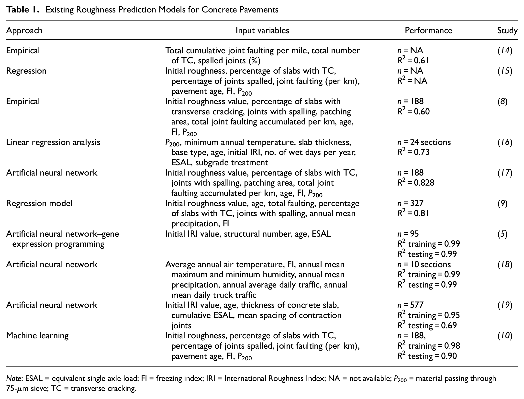
Note: ESAL = equivalent single axle load; FI = freezing index; IRI = International Roughness Index; NA = not available; P₂₀₀ = material passing through 75-µm sieve; TC = transverse cracking.

The sample size, number of variables used, and performance of the model in these studies have been analyzed in detail. Although most of these models have performed well with high-performance indices, there are a few limitations, as analyzed and discussed:

Sample size or number of data points. A ML model’s performance is highly associated with the sample population. The larger the sample size of the training data, the more robust and reliable the model. The maximum number of data points or largest sample size used in all the studies is 577 and the minimum is less than a hundred.

Technique or method. Most of the models shown in Table 1 were based on simple regression or traditional ML, such as random forest, XG Boost, or neural networks. There are very few studies where advanced optimization methods were used for model development.

In this study, the limitations of the previous studies discussed in this section have been addressed. First, the issue of a smaller number of data points was overcome by maximizing the sample size in this research. Additionally, all the relevant feature variables that could contribute to predicting the IRI were selected to ensure a comprehensive model. A total of 920 observations were used for the model development, of which 80% were used for training and the rest were used for testing.

To enhance the robustness and practicality of the model, the research went beyond conventional ML methods by incorporating PINNs along with the Optuna framework. This approach allowed for the incorporation of physical principles and constraints in the ML model, resulting in a more reliable and interpretable analysis. The combination of physics-driven ML with novel optimization techniques was intended to achieve a more refined and accurate prediction model. The relative importance of variables to the final IRI has been identified through sensitivity analysis.

Data Preparation

Roughness, in general, is a function of many variables in concrete pavements. The MEPDG roughness prediction model, as shown in Equations 1 and 2, considered eight parameters for predicting roughness, including initial roughness, slabs with transverse cracking (as a percentage), joints with spalling of all severities (as a percentage), patching area of all severities, total joint faulting accumulated, and site factor. Site factor is again a function of pavement age, freezing index, and the percentage subgrade passing through a 75-µm sieve. All these parameters were extracted from the LTPP repository, which includes 10 states with 48 sections. The total number of data points used in this study was 923, of which 80% were used for training. The samples were extracted from periods in which no maintenance or rehabilitation was undertaken, to ensure the unbiased nature of the model. The LTPP repository determines pavement roughness, using the IRI, for both left- and right-wheel tracks. In this study, the roughness considered for each section is the maximum value of the right- and left-wheel track IRI. Using the maximum IRI provides a more conservative estimate of road roughness than using the average or minimum IRI.

The MEPDG model for calculating the IRI of a JPCP is represented as ( 6 )

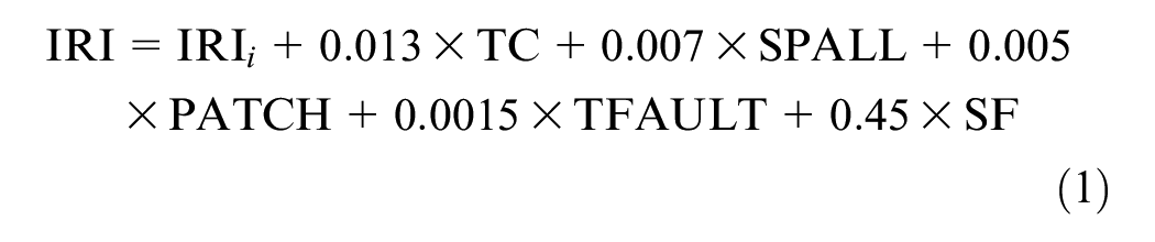
\begin{matrix} IRI & = {IRI}_{i} + 0.013 \times TC + 0.007 \times SPALL + 0.005 \\ \times PATCH + 0.0015 \times TFAULT + 0.45 \times SF \end{matrix}

(1)

where IRI_i is the initial smoothness measured as IRI, expressed in meters per kilometer; TC is the percentage of slabs with transverse cracking (all severities); SPALL is the percentage of joints with spalling (all severities); PATCH is the pavement surface area with flexible and rigid patching (all severities), expressed as a percentage; TFAULT is the total joint faulting cumulated per kilometer, measured in millimeters; and SF is the site factor, which is calculated as

SF = Age \times (1 + FI) \times (1 + P_{200}) / 10^{6}

(2)

where Age is the pavement age in years; FI is the freezing index, measured in degrees Celsius days; and P₂₀₀ is the percentage of subgrade material passing through a 75-µm sieve.

All the variables were statistically analyzed to derive indicators, such as average, median, or standard deviation. All these details are summarized in Table 2 for the extracted dataset. In the table, variables IRI_i, SPALL, PATCH, FAULT, FI, P₂₀₀, and IRI have positive skewness values, indicating a right-skewed distribution. This means that these variables have more data points toward the lower end of the range and fewer points toward the higher end. They also have positive kurtosis values, indicating distributions with heavier tails and a more peaked shape. These indicators aid in comprehending the dataset from both qualitative and quantitative perspectives.

Table 2.

Statistical Indicators for the Independent Variables Used in This Study

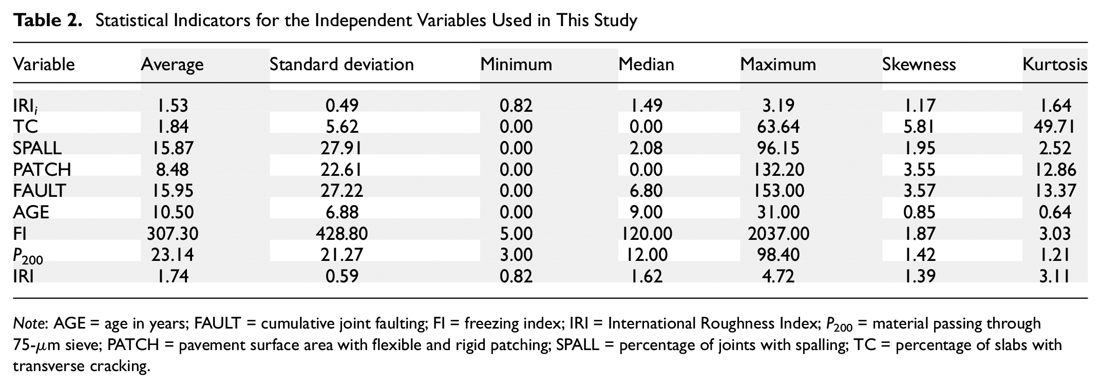
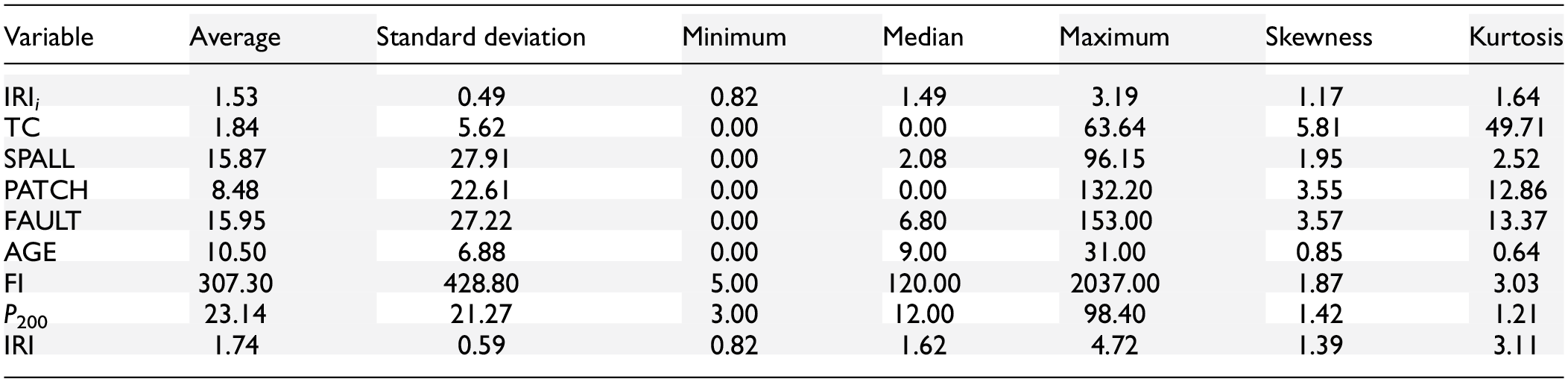
Note: AGE = age in years; FAULT = cumulative joint faulting; FI = freezing index; IRI = International Roughness Index; P₂₀₀ = material passing through 75-µm sieve; PATCH = pavement surface area with flexible and rigid patching; SPALL = percentage of joints with spalling; TC = percentage of slabs with transverse cracking.

A correlogram of all the variables in this study is presented in Figure 1. It is used to visualize the linear relationships between different variables and identify patterns in the data. In the figure, the higher the correlation, the darker the color. A positive correlation is represented by the color red, while a negative correlation is denoted by the color blue. This figure shows that there is a high correlation between the initial roughness and current roughness followed by freezing index, whereas transverse cracking and patching show the least correlation with current roughness. It can also be observed that the proportion passing through a 75-µm sieve shows a negative correlation with all other variables.

Figure 1.

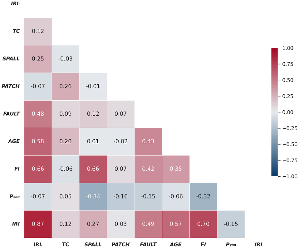
Correlogram of all the variables used in this study.

The MEPDG model assumes independence for the various parameters used for predicting pavement roughness. This assumption implies that the factors influencing roughness, such as initial roughness, transverse cracking, spalling, patching, total joint faulting, and site factors, are considered to be independent variables. However, the analysis, as depicted in Figure 1, reveals correlations between these variables, suggesting a departure from the assumed independence.

Figure 1 illustrates noticeable correlations between certain variables, notably a high correlation between initial roughness and current roughness, as well as with the freezing index. Conversely, some variables, such as transverse cracking and patching, exhibit smaller correlations with current roughness. The presence of these correlations implies that the influence of certain parameters on pavement roughness might be interconnected or influenced by shared underlying factors. Such interdependencies might introduce complexities not fully captured by the MEPDG model, potentially affecting the accuracy of roughness predictions.

Once the dataset had been extracted, it could be used to train the model for prediction. Typically, in this study, the dataset was divided into training and test sets, with a split ratio of 80:20. The model was trained using the training set, and the performance of the trained model was evaluated using the test set. The dataset was partitioned into the desired proportions and a histogram of the target variable, faulting, for both sets, was plotted and distributions were compared. In the split used for this study, as shown in Figure 2, the distributions are similar, giving confidence that the split is likely to be of good quality.

Figure 2.

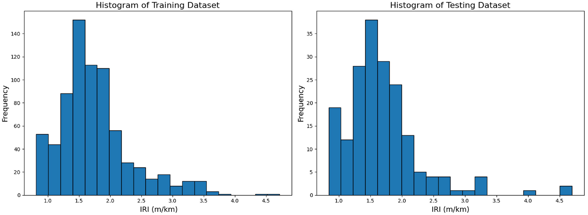
Histogram of the training and testing datasets.

PINNs

It is important to understand neural networks to gain insight into PINNs. DNNs replicate the functioning of the human brain, empowering computer programs to recognize patterns and address fundamental challenges in artificial intelligence (AI), ML, and deep learning ( 20 ). A typical neural network comprises input, hidden, and output layers. In a neural network’s hidden layer, each node or neuron is connected to others, having its unique set of weights and a threshold. When a node’s output exceeds the threshold, it becomes activated and passes information to the next layer. However, if the output does not meet the threshold, no data are transmitted to the subsequent layer. Once the network is trained, it can make predictions based on inputs without explicitly understanding the relationships between them. This prediction process does not rely on specific algorithms or expertise in the subject matter ( 21 ). Training is achieved by applying input vectors and adjusting network weights through a predefined process until a consistent output is obtained.

As presented in the neuron function diagram of a DNN in Figure 3, X₁ to X_n are the first to nth input variables, W₁ to W_n are the weights for the input features, b is a fixed number (the bias), and F is a transfer function. The weights W_i and bias (b) in neurons are established through a suitable optimization technique ( 22 ). Activation functions (AFs) are utilized by DNNs in the hidden layers to perform complicated computations and then relay the outcomes to the output layer.

Figure 3.

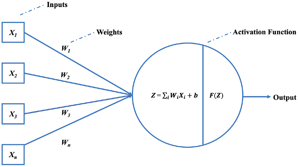
Architecture of a deep neural network.

The main purpose of AFs is to incorporate non-linear characteristics in the network. They transform the linear input signals of nodes into non-linear output signals, allowing deep networks to learn high-order polynomials with degrees greater than one. Additionally, AFs are differentiable, enabling the use of backpropagation for training. In this study, the rectified linear unit (ReLU) function was utilized. This function is a rapid-learning activation function that ensures robust and exceptional performance. Compared with other AFs, the ReLU function provides significantly superior deep learning performance and generalization ( 23 ).

The DNN architecture focuses on predicting roughness (measured in meters per kilometer) in jointed concrete pavements, where the output variable is roughness. Within this architecture, several parameters are employed to adjust the parameters of the deep learning or ML model, including the learning rate and weights, aiming to minimize losses. As a part of the optimization process, it is crucial to estimate the error for the current state of the model repeatedly. To update the weights and reduce the loss in the next evaluation, an error function, also called a loss function, must be selected. This function can be used to estimate the loss of the model. The loss function is fundamental to the training process of the neural network. During training, the model iteratively adjusts its parameters (weights and biases) to minimize the overall loss. The mean square loss function used in this study is generally used in regression tasks.

Neural networks have demonstrated remarkable versatility in predicting various distress types within pavement engineering. Researchers have leveraged the power of these computational models to address critical challenges, such as faulting, roughness, and cracking. The ability of neural networks to discern intricate patterns in pavement conditions has led to significant advances in distress prediction models. Studies focused on faulting have explored the nuanced relationships between input parameters and the occurrence of this specific pavement issue ( 24 , 25 ). Similarly, investigations into roughness have utilized neural networks to unravel the complex interplay of factors influencing pavement surface irregularities ( 18 , 26 ). Moreover, cracking, a common concern in pavement degradation, has been the subject of extensive research employing neural networks to capture the underlying dynamics contributing to crack initiation and propagation ( 27 – 29 ). These applications extend beyond isolated distress predictions, as researchers have also integrated neural network predictions in comprehensive assessments of pavement condition, introducing such indices as the Pavement Condition Index and the overall condition index ( 30 – 33 ). This integration showcases the broader impact of neural networks in providing holistic evaluations of pavement performance, offering valuable insights for maintenance and rehabilitation strategies.

Despite the undeniable advantages of DNNs, there are some concerns about the deployment of neural networks. Critics often point to the inherent black-box nature of these models, where it becomes challenging to interpret the underlying mechanisms driving their predictions. This lack of transparency can be problematic, especially in critical applications where users require clear explanations for a model’s decisions. To address these concerns, researchers have been actively exploring physics-based ML approaches. These methods aim to incorporate domain-specific knowledge and physical principles in the design of ML models. By integrating human-understandable concepts in the learning process, these ML models will provide more interpretable outputs and build trust with users.

In pavement engineering, mechanistic or mechanistic-empirical models have historically been dominant, owing to their interpretability, and there is now a growing interest in combining these models with the power of ML. DNNs that adhere to fundamental physical laws have been implemented, providing insights into the structural behavior, material properties, and failure modes of complex civil engineering systems.

While PINNs are often employed to solve partial differential equations by incorporating physical constraints directly into the neural network architecture, they can also be adapted to handle other types of equation or constraints with domain knowledge ( 34 ). The PINN architecture consists of two main components, where the first one is the neural network and the second one is the physics-based loss function, as shown in Figure 4. The additional component in the architecture, compared with regular DNNs, is the physics-based loss function. The data-driven terms learn the relationships between input features and target variables from the data, while the physics-driven terms enforce the known or approximated physical constraints in the problem.

Figure 4.

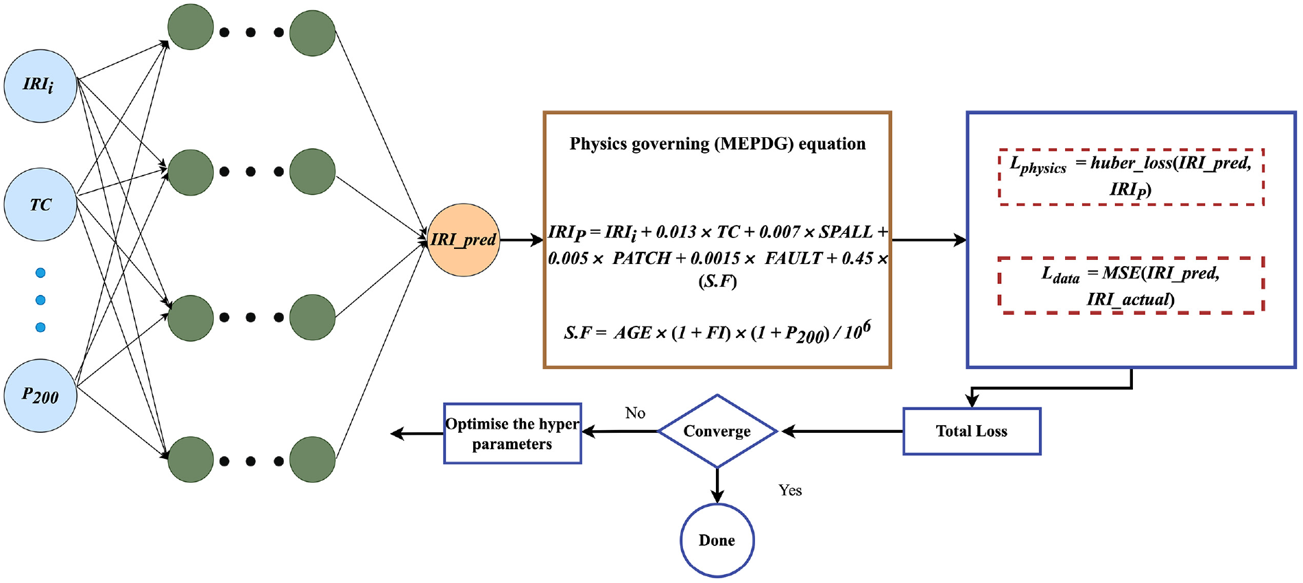
Typical visualization of physics informed neural network (PINN) architecture.

The MEPDG equation is widely used to predict the roughness of JPCPs. Taking the leverage of an established equation, and exploiting the computational performance of neural networks, a PINN is designed to compute the physics loss component by the Huber loss of the predicted IRI and the IRI calculated using the neural networks. The overall loss is computed as the sum of the weighted averages of the data fidelity loss and physics loss, as

Loss = a \times L_{data} + b \times L_{physics}

(3)

In Equation 3, L_data is also known as the data fidelity loss, and is measured as a function of mean squared error. It measures the discrepancy between the IRI predicted by the neural networks and the actual measured roughness value.

The variable L_physics is the physics-based loss function that is used as a constraint in PINNs. The major goal is to use neural networks to learn the solution to a physical problem directly from data while incorporating the governing physics equations as constraints. The overall loss is calculated as the Huber loss of the IRI predicted by the neural networks and the IRI calculated using the MEPDG equation.

In Equation 3, a and b are the weights assigned to optimize the overall loss function. These parameters allow us to control the importance of fitting the data versus adhering to the physics. In this study, after several iterations with various combinations, 0.75 and 0.25 were found to be optimum values for this model, for a and b, respectively.

To optimize the weighting of the losses, a range of combinations was explored to compute the final loss after training. This optimization process is visualized in Figure 5, where each data point represents a unique combination of a and b, and the total loss is plotted against a. Notably, each point is color-coded according to its corresponding b value.

Figure 5.

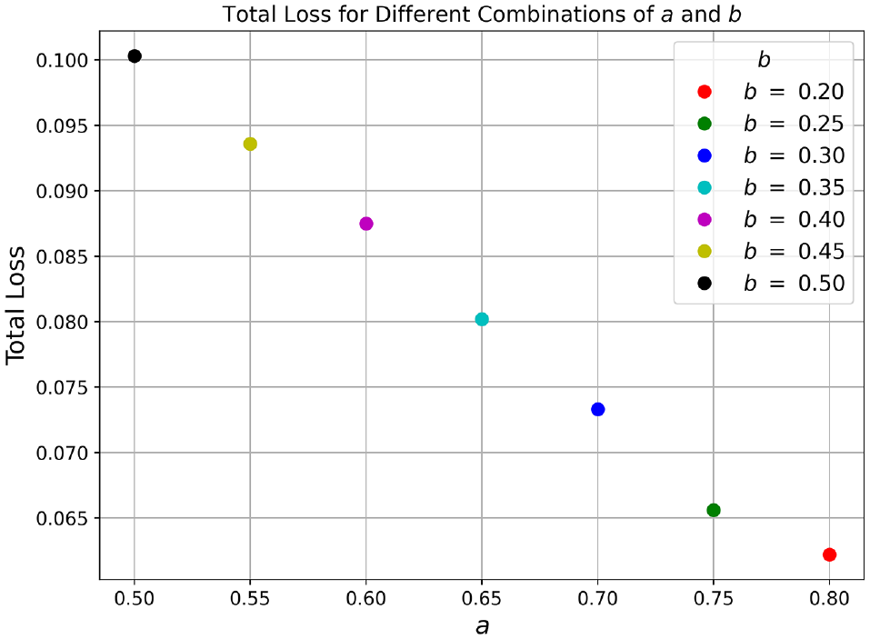
Line plot depicting the losses computed after training across various combinations of a and b.

It is evident from the plot that, as b decreases, the overall loss decreases as well. However, beyond a certain threshold (b = 0.25), the rate of decrease in loss diminishes. To achieve a balance between optimizing the losses and maintaining the relevance of the physics-based loss, b was chosen to be 0.25, with a corresponding weight of 0.75 assigned to a. These values were selected to ensure effective loss optimization while preserving the significance of the physics governing equation.

There have been several studies of DNN implementation in civil and pavement engineering. However, there are limited studies where PINNs have been utilized in the field of civil engineering. Physics-based ML was applied in structural health monitoring of civil structures ( 35 , 36 ), materials modeling ( 37 ), and structural mechanics ( 38 ).

Optuna Framework

Optuna is an optimization framework that exploits the concept of sequential model-based optimization to efficiently search for the optimal set of hyperparameters for a ML model. This method is based on the idea of using surrogate models to model the complex relationship between hyperparameters and a model’s performance. Instead of exhaustively searching the entire hyperparameter space, Optuna uses probabilistic models to guide the search more efficiently, focusing on promising regions of the space ( 39 ). There are very few studies where Optuna was utilized for civil engineering applications, although in one study it was implemented to tune the hyperparameters for lidar odometry estimation ( 40 ).

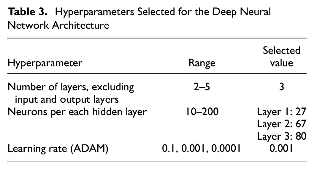
The major hyperparameters optimized in this study are the number of hidden layers, the number of neurons in each hidden layer, and the learning rate of the Adaptive Moment Estimation (ADAM) optimizer. The primary objective of the library used in this study is to minimize the error by iteratively suggesting new hyperparameter configurations based on the results of previous evaluations. The objective function for each set of hyperparameters in the initial trials records the R² score associated with each hyperparameter configuration. Optuna iteratively performs the optimization loop until a stopping criterion is met. In this study, the optimization criterion was the maximum number of iteration trials namely, 100. Table 3 presents the range of values explored for each hyperparameter and the selected value for the final configuration.

Table 3.

Hyperparameters Selected for the Deep Neural Network Architecture

Hyperparameter	Range	Selected value
Number of layers, excluding input and output layers	2–5	3
Neurons per each hidden layer	10–200	Layer 1: 27 Layer 2: 67 Layer 3: 80
Learning rate (ADAM)	0.1, 0.001, 0.0001	0.001

Model Development

In this section, the process of training, tuning, and optimization of the models, and assessment of the models against the training data, is explained. Google Colaboratory, an online platform that provides a Jupyter-like environment for running and executing code was used in this study. It is particularly useful for ML and data science tasks, as it offers access to high-performance computing resources, such as graphics processing units (GPUs) and tensor processing unit (TPUs). Figure 6 is a flowchart of the model development and validation process.

Figure 6.

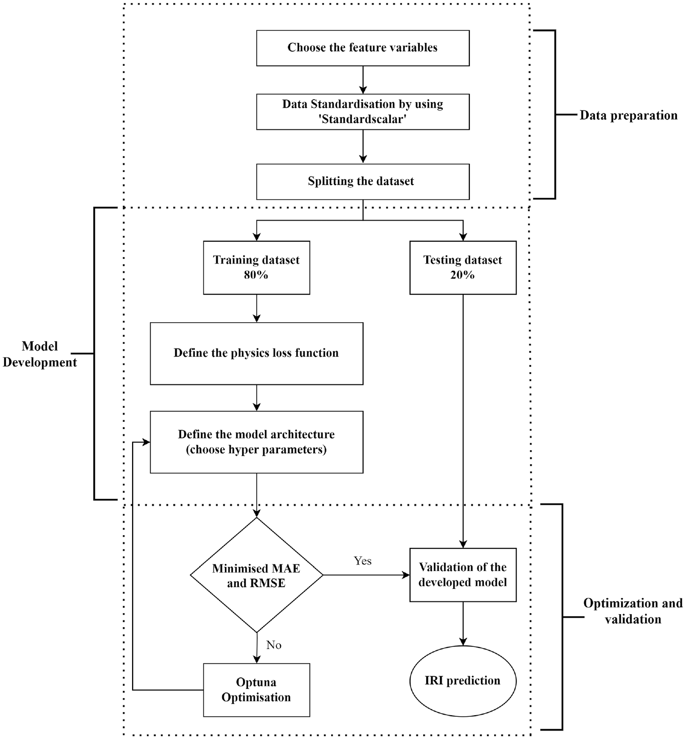
Flowchart explaining the model development of physics informed neural networks in this study.

The efficacy of a ML model is contingent on the caliber of the data used for its training. Therefore, it is essential to properly pre-process the data before using the dataset to train the model. Data pre-processing involves transforming or encoding the dataset so that it can be easily understood by the machine. In this study, the data are pre-processed and transformed to ensure that all variables are considered equally by the ML model. This is important because variables measured at different scales might not contribute equally to the model’s ability to fit and learn. For example, in the dataset used in this research, the initial IRI is in the range of 0.82 to 3.19, while the freezing index ranges from 5 to 2037. If a ML algorithm based on the Euclidean distance method is used, the initial IRI will be given less weight than the freezing index.

To tackle this concern, a feature-wise normalization technique known as MinMax Scaler, was implemented, using the scikit-learn libraries, on the input features before fitting the model. This process guarantees that all features are transformed into the range [0,1], with 0 and 1 as the minimum and maximum values for each feature or variable, respectively:

x_{scaled} = \frac{x - x_{min}}{x_{max} - x_{min}}

(4)

where x_scaled is the calculated normalized value, x is the actual value, x_min is the minimum value, and x_max denotes the maximum value of the required variable.

This leads to an improvement in the efficiency and effectiveness of algorithm execution. Since the dataset is already of a reduced size, the complex calculations required to enhance the algorithms can be performed much faster. For model training, the pre-processed dataset is divided into training and testing datasets, with a ratio of 80% for training and 20% for testing. This split is accomplished using the train_test_split function from the scikit-learn library, which randomly assigns rows of the dataset to the respective proportions. The performance metrics for evaluating models used in this study were the R² score (coefficient of determination), mean absolute error (MAE), mean squared error (MSE), and root mean squared error (RMSE).

The neural network architecture was initially defined with two input layers and 16 neurons in each hidden layer. The ReLU activation function was used in this study, owing to its simplicity and computational efficiency. To fit the model, the powerful ADAM optimizer, with a learning rate of 0.01, was deployed. With this architecture and physics constraint, the model was trained with 100 epochs. Then the same model was validated using the testing dataset. The scatter plots of the training and testing datasets were plotted for the predicted and true values of IRI, as shown in Figure 7. The value of R² for the testing dataset for the initial PINNs is 0.85 and the RMSE is 0.232 m/km. The prediction performance of the model will be improved by optimizing the hyperparameters.

Figure 7.

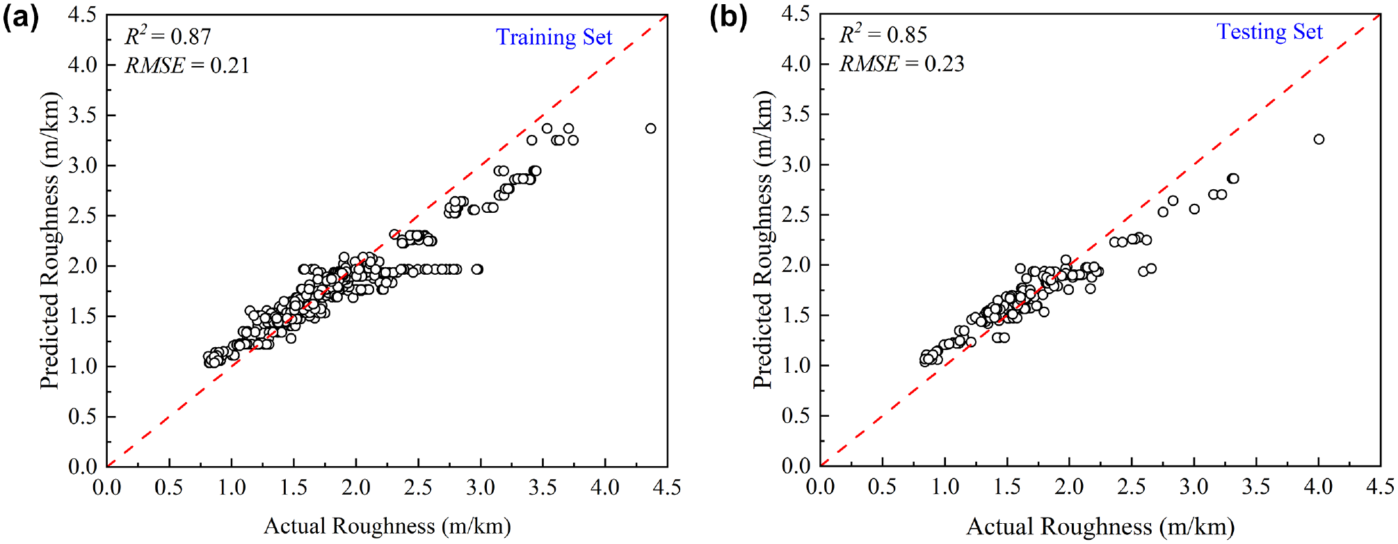
Predicted versus actual values of International Roughness Index (meters per kilometer) using the initial physics informed neural network model: (a) training dataset; (b) testing dataset.

Although the performance of the initial PINN is good, the model can be further fine-tuned by optimizing the hyperparameters within the neural network architecture. In this study, a novel tuning method, Optuna framework, was deployed to tune the hyperparameters. When the tuning was performed, by aiming to find the hyperparameters that led to the highest value of R², indicating the best model performance on the testing set, the hyperparameters selected after 100 iterations were three hidden layers, with the numbers of neurons being 27, 67, and 80, respectively. The learning rate selected for the ADAM optimizer was 0.001. These parameters were obtained after Optuna tried different combinations of hyperparameters and evaluated how well the model performed with each combination. The goal was to maximize R², which tells how close the predictions are to the actual roughness values. After evaluating various combinations, the best hyperparameters that led to the highest value of R² were selected. When the model was compiled using these parameters, the performance of the model was further enhanced. The coefficients of determination of the testing and training datasets for the optimized model were 0.92 and 0.90, respectively, whereas the RMSEs for the training and test datasets were 0.162 and 0.189 m/km, respectively. This means that the optimized model shows an improvement of around 18.5% compared with the basic model, based on the RMSEs. Scatter plots of the training and testing datasets were produced for the predicted and measured values of IRI when tuned using the Optuna framework, as shown in Figure 8.

Figure 8.

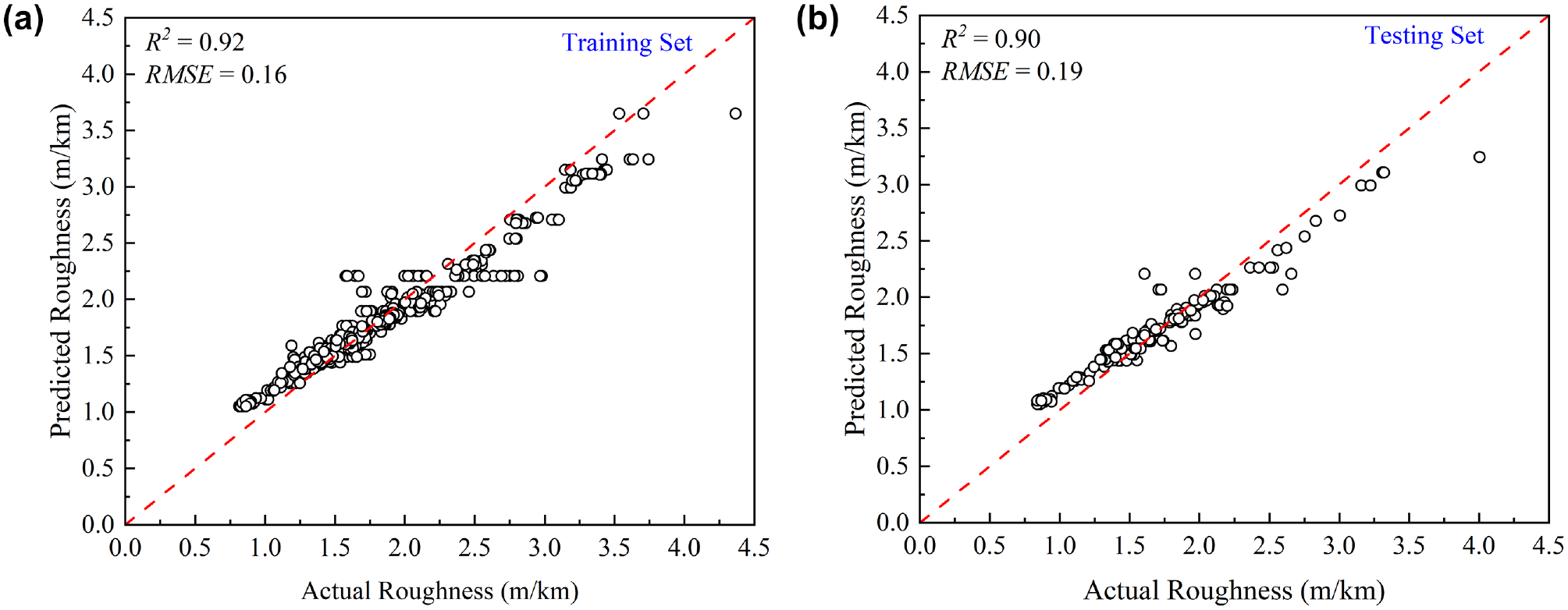
Predicted versus actual values of International Roughness Index (meters per kilometer) using the optimized physics informed neural network model: (a) training dataset; (b) testing dataset.

Sensitivity Analysis

To understand the deeper behavior of the model, and its relationship with the variables used, sensitivity analysis was conducted in this study. It was conducted on all the input factors that are most responsible for increasing roughness, that is, initial IRI, transverse cracking, spalling, faulting, and patching. In this section, the effect of change in these features on the prediction of the final predicted IRI is estimated. The sensitivity analysis was conducted for the PINN model with the best performing parameters. With a total of eight input features in use, the analysis involved a systematic variation of each input variable’s value, while maintaining the other variables at their mean values across 10 rows. For example, to conduct the sensitivity analysis for the initial IRI, the seven other input variables were assigned their mean values across 10 rows while the initial IRI value was varied from its minimum value to its maximum in 10 steps. Subsequently, the model was employed to predict roughness (IRI) at each step to produce Figure 9a. To produce Figure 9b, transverse cracking was varied from its minimum value to its maximum in 10 steps, keeping other variables the same in each row as their average values. A similar method was followed to conduct the sensitivity analysis for spalling, patching, and faulting, as illustrated in Figure 9, c to e .

Figure 9.

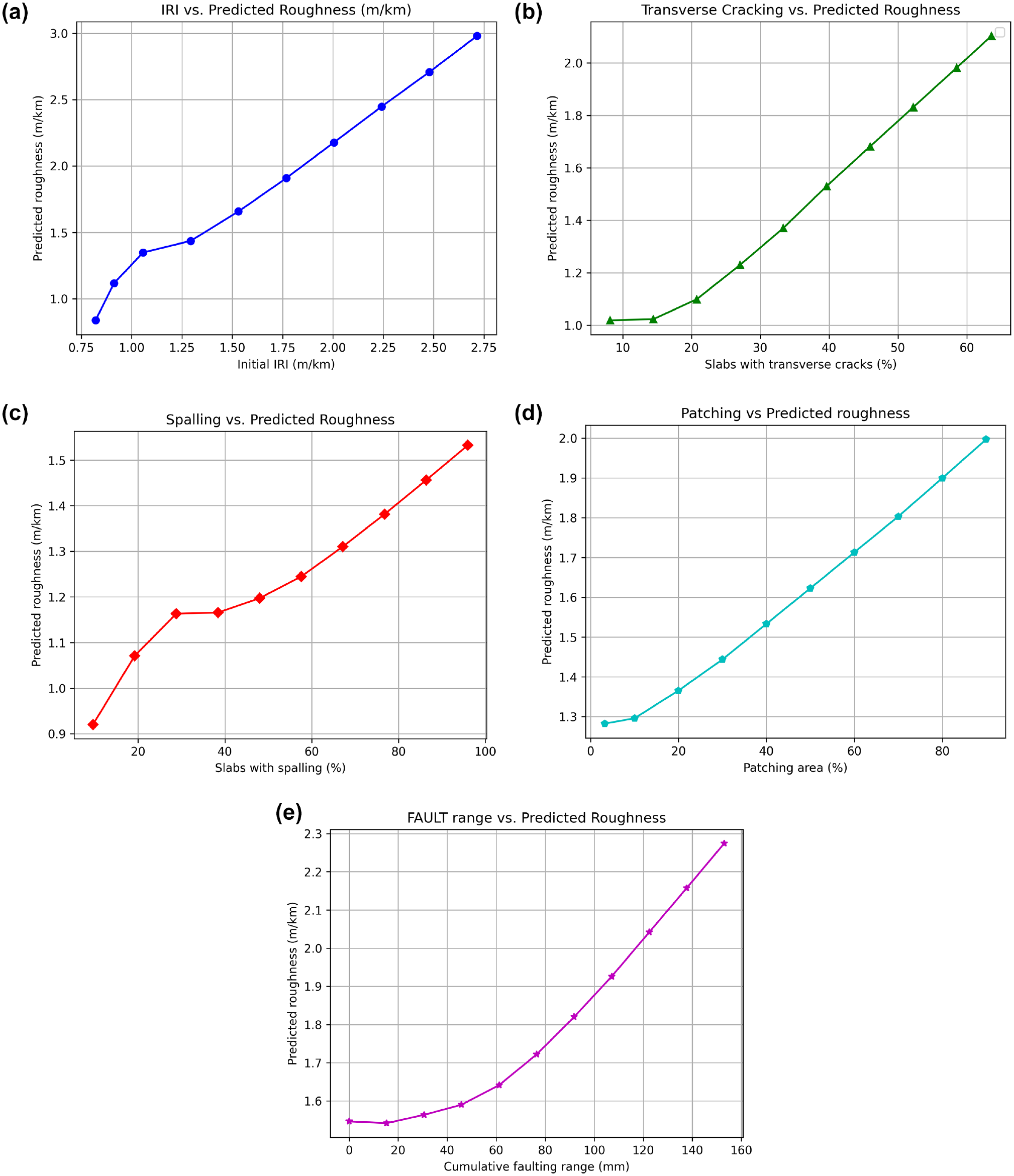
Sensitivity analysis of features used in this study: (a) initial International Roughness Index (IRI); (b) transverse cracks; (c) spalling; (d) patching; (e) cumulative faulting.

These figures show that, with an increase in the value of feature variables, the overall roughness increases. It can also be observed that the rate of increment for the initial IRI and transverse cracking is greater than that for other variables. Sensitivity analysis demonstrates that the model behaves consistently and that it can make reliable predictions with the new data.

Performance Metrics

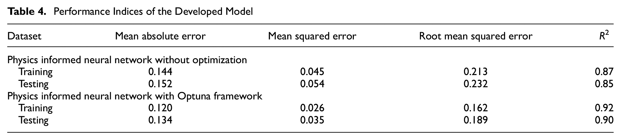
To build and deploy a generalized model that performs well, it is necessary to evaluate the model using various metrics. This helps to optimize the model’s performance, fine-tune it, and ultimately produce better results. The evaluation performance metrics for the basic PINN and optimized PINN models were calculated in this study. These indices were calculated for the training and testing data and are summarized in Table 4. The MAE in the Optuna PINN model is smaller than that in the basic model. Other indices have also confirmed that the optimized method is the best performing, with the smallest errors for both training and testing datasets.

Table 4.

Performance Indices of the Developed Model

Dataset	Mean absolute error	Mean squared error	Root mean squared error	R ²
Physics informed neural network without optimization
Training	0.144	0.045	0.213	0.87
Testing	0.152	0.054	0.232	0.85
Physics informed neural network with Optuna framework
Training	0.120	0.026	0.162	0.92
Testing	0.134	0.035	0.189	0.90

Conclusions

Roughness is an important factor in assessing the ride quality and serviceability of concrete pavements. Therefore, it is important to accurately predict the roughness of concrete pavement. This paper proposes a novel method for predicting roughness by utilizing data including spalling, transverse cracking, faulting, patching, freezing index, initial roughness, and age. A novel approach that combines physics-driven ML with the LTPP dataset was implemented to predict pavement roughness. This innovative method harnesses the benefits of scientific computing and incorporates physical constraints (the MEPDG equation) for improved predictive accuracy.

Based on this study, it is understood that data pre-processing and standardization techniques have contributed significantly to achieving good prediction results. The basic PINN model, with two hidden layers and 16 nodes in each hidden layer, produced reasonably good results. The coefficient of determination of this model was 0.85 and the MAE was 0.152 m/km. When optimized using Optuna, the performance further increased to give a coefficient of determination of 0.90 and an MAE of 0.134 m/km. The hyperparameters selected after tuning with Optuna are three hidden layers, with 27, 67, and 80 neurons, respectively. From sensitivity analysis of feature variables, it can be understood how the prediction results vary with the increase in the feature variables, when the other parameters are kept constant.

By harnessing this comprehensive dataset, infrastructure managers and road agencies can gain a nuanced understanding of the factors influencing pavement roughness. The predictive accuracy is further strengthened by the incorporation of physical constraints through the MEPDG equation, ensuring a robust and scientifically grounded methodology. Importantly, while this study focuses on roughness prediction, its broader implications suggest that PINNs hold significant potential for predicting various types of distress in pavements. End-users can leverage this methodology, not only for roughness assessments but also for proactive monitoring of other critical pavement conditions.

This study demonstrates that PINNs are a reliable and robust approach for developing accurate roughness prediction models for JPCPs by combining both physical constraints and neural networks. The study is not intended as a sponsored effort to update the existing IRI model but rather to showcase the potential of PINNs in its prediction. The findings also strongly suggest that PINNs hold immense potential for predicting other forms of distress in pavements as well. Moreover, the positive outcomes of this research highlight how continuous advancements in PINN methodologies can effectively address numerous challenges, leading to noteworthy progress in the application of PINNs in the field of pavement engineering.

Footnotes

Author Contributions

The authors confirm contribution to the paper as follows: study conception and design: S. K. Pasupunuri, L. Li; data collection: S. K. Pasupunuri; analysis and interpretation of results: S. K. Pasupunuri, N. Thom, L. Li; draft manuscript preparation: S. K. Pasupunuri, N. Thom. All authors reviewed the results and approved the final version of the manuscript.

Declaration of Conflicting Interests

The author(s) declared no potential conflicts of interest with respect to the research, authorship, and/or publication of this article.

Funding

The author(s) disclosed receipt of the following financial support for the research, authorship, and/or publication of this article: This research is supported by funding from National Highways, UK, to the University of Nottingham, UK.

ORCID iDs

Nick Thom

Linglin Li

Data Accessibility Statement

The datasets used for this study and the source code are available from the corresponding author on reasonable request.

References

Huang

Y. H.

Pavement Analysis and Design. Pearson/Prentice Hall, Hoboken, NJ, 2004, p. 775.

Haas

Hudson

W. R.

Pavement Asset Management. Scrivener Publishing, Beverly, MA, 2015.

Thom

Principles of Pavement Engineering. Vol. 1, ICE Publishing, Westminster, London, 2014, p. 423.

Delatte

N. J.

Concrete Pavement Design, Construction, and Performance, 2nd ed. CRC Press, Boca Raton, FL, 2014.

Mazari

Rodriguez

D. D.

Prediction of Pavement Roughness Using a Hybrid Gene Expression Programming-Neural Network Technique. Journal of Traffic and Transportation Engineering (English Edition), Vol. 3, No. 5, 2016, pp. 448–455.

Georgiou

Plati

Loizos

Soft Computing Models to Predict Pavement Roughness: A Comparative Study. Advances in Civil Engineering, 2018, Vol. 2018, pp. 1–8.

Damirchilo

Hosseini

Mellat Parast

Fini

E. H.

Machine Learning Approach to Predict International Roughness Index Using Long-Term Pavement Performance Data. Journal of Transportation Engineering, Part B: Pavements, Vol. 147, No. 4, 2021, p. 04021058.

Titus-Glover, L., and M. I. Darter. NCHRP Appendix PP. Guide for MEPDG Appendix PP: Smoothness Prediction for Rigid Pavements. Transport Research Board, IL, 2003.

Naguib

A. M.

El-Badwy

S. M.

Ibrahim

M. H.

International Roughness Index Predictive Model for Rigid Pavements Based on LTPP Data. Mansoura Engineering Journal, Vol. 40, No. 2, 2015, pp. 30–38.

10.

Wang

Zhou

Sabri

M. M. S.

Huang

A Comparative Study of AI-Based International Roughness Index (IRI) Prediction Models for Jointed Plain Concrete Pavement (JPCP). Materials, Vol. 15, No. 16, 2022, p. 5605.

11.

Suliman

A. M.

Awed

A. M.

Abd El-Hakim

R. T.

El-Badawy

S. M.

International Roughness Index Prediction for Jointed Plain Concrete Pavements Using Regression and Machine Learning Techniques. Transportation Research Record: Journal of the Transportation Research Board, 2024. 2678: 235–250.

12.

Park

Thomas

N. E.

Lee

K. W.

Applicability of the International Roughness Index as a Predictor of Asphalt Pavement Condition 1. ASCE Journal of Transportation Engineering, Vol. 133, No. 12, 2007, pp. 706–709.

13.

IRC:SP:16-2019. Guidelines on Measuring Road Roughness and Norms. Indian Roads Congress, New Delhi, 2019.

14.

H. T.

Smith

K. D.

Darter

M. I.

Jiang

Khazanovich

Performance of Concrete Pavements, Volume III: Improving Concrete Pavement Performance FHWA-RD-95-111. https://trid.trb.org/view/484795. Accessed August 2, 2021.

15.

Hoerner

T. E.

Darter

M. I.

Khazanovich

Titus-Glover

Smith

K. L.

Improved Prediction Models for PCC Pavement Performance-Related Specifications, Volume I: Final Report. https://www.fhwa.dot.gov/publications/research/infrastructure/pavements/pccp/pavespec/00130.pdf. Accessed August 2, 2021.

16.

Felker

Hossain

Najjar

Barezinsky

Roughness Progression Model on Kansas PCC Pavements. Proc., Mid-Continent Transportation Research Symposium, Ames, IA, 2003.

17.

Abd El-Hakim

El-Badawy

International Roughness Index Prediction for Rigid Pavements: An Artificial Neural Network Application. Advanced Materials Research, Vol. 723, 2013, pp. 854–860.

18.

Hossain

Gopisetti

L. S. P.

Miah

M. S.

Artificial Neural Network Modelling to Predict International Roughness Index of Rigid Pavements. International Journal of Pavement Research and Technology, Vol. 13, No. 3, 2020, pp. 229–239.

19.

Sultana

Najjar

Yasarer

Uddin

Barros

International Roughness Index Model for Jointed Reinforced Concrete Highway Pavements: An Artificial Neural Network Application. Proc., 11th International Conference on the Bearing Capacity of Roads, Railways and Airfields, Volume 3, Trondheim, Norway, CRC Press, Boca Raton, FL, 2022, pp. 246–255.

20.

Sutton

R. S.

Barto

A. G.

Reinforcement Learning: An Introduction. MIT Press, Cambridge, MA, 1998.

21.

Bishop

C. M.

Pattern Recognition and Machine Learning. Springer, New York, NY, 2006.

22.

Vandeginste

B. G. M.

Massart

D. L.

Buydens

L. M. C.

de Jong

Lewi

P. J.

Smeyers-Verbeke

Artificial Neural Networks. In Data Handling in Science and Technology, Elsevier, Amsterdam, 1998. Vol. 20, part 2, pp. 649–699.

23.

Goodfellow

Bengio

Courville

Deep Learning. MIT Press. https://www.deeplearningbook.org/. Accessed July 27, 2023.

24.

DeSantis

J. W.

Vandenbossche

J. M.

Alland

Harvey

Development of Artificial Neural Networks for Predicting the Response of Bonded Concrete Overlays of Asphalt for Use in a Faulting Prediction Model. Transportation Research Record: Journal of the Transportation Research Board, 2018. 2672: 360–370.

25.

Ehsani

Moghadas Nejad

Hajikarimi

Developing an Optimized Faulting Prediction Model in Jointed Plain Concrete Pavement Using Artificial Neural Networks and Random Forest Methods. International Journal of Pavement Engineering, Vol. 24, No. 2, 2022, p. 2057975.

26.

Chandra

Chalumuri

Bhart

A. K.

Kangadurai

Relationship Between Pavement Roughness and Distress Parameters for Indian Highways. ASCE Journal of Transportation Engineering, Vol. 139, No. 5, 2013, pp. 467–475.

27.

Yang

J. J.

Gunaratne

Application of Neural Network Models for Forecasting of Pavement Crack Index and Pavement Condition Rating. Development of Civil and Environmental Engineering, University of South Florida, Tampa, 2003.

28.

G. X.

B. L.

Yang

Huang

Pavement Crack Detection Method Based on Deep Learning Models. Wireless Communications and Mobile Computing, Vol. 2021, 2021, pp. 1–3.

29.

Pasupunuri

S. K.

Thom

Use of Machine Learning Algorithms for Predicting the Transverse Cracking in Jointed Plain Concrete Pavements. Proc., Airfield and Highway Pavements, Austin, TX, American Society of Civil Engineers, Reston, VA, 2023, pp. 172–184.

30.

Alharbi

Predicting Pavement Performance Utilizing Artificial Neural Network (ANN) Models. https://lib.dr.iastate.edu/etd/16703.

31.

Thube

D. T.

Artificial Neural Network (ANN) Based Pavement Deterioration Models for Low Volume Roads in India. International Journal of Pavement Research and Technology, Vol. 5, No. 2, 2012, pp. 115–120.

32.

Guo

Zhao

Gregory

Kirchain

A Weighted Multi-Output Neural Network Model for the Prediction of Rigid Pavement Deterioration. International Journal of Pavement Engineering, Vol. 23, No. 8, 2022, pp. 2631–2643.

33.

Issa

Samaneh

Ghanim

Predicting Pavement Condition Index Using Artificial Neural Networks Approach. Ain Shams Engineering Journal, Vol. 13, No. 1, 2021, p. 101490.

34.

Raissi

Perdikaris

Karniadakis

G. E.

Physics-Informed Neural Networks: A Deep Learning Framework for Solving Forward and Inverse Problems Involving Nonlinear Partial Differential Equations. Journal of Computational Physics, Vol. 378, 2019, pp. 686–707.

35.

Zheng

Moosavi

Akbarzadeh

Machine Learning Assisted Evaluations in Structural Design and Construction. Automation in Construction, Vol. 119, 2020, p. 103346.

36.

Chen

Liu

Probabilistic Physics-Guided Machine Learning for Fatigue Data Analysis. Expert Systems with Applications, Vol. 168, 2021, p. 114316.

37.

Liu

Wang

Multi-Fidelity Physics-Constrained Neural Network and Its Application in Materials Modeling. Journal of Mechanical Design, Vol. 141, No. 12, 2019, p. 121403.

38.

Sadoughi

Physics-Based Convolutional Neural Network for Fault Diagnosis of Rolling Element Bearings. IEEE Sensors Journal, Vol. 19, No. 11, 2019, pp. 4181–4192.

39.

Akiba

Sano

Yanase

Ohta

Koyama

Optuna: A Next-Generation Hyperparameter Optimization Framework. Proc., ACM SIGKDD International Conference on Knowledge Discovery and Data Mining, Anchorage, AK, Association for Computing Machinery, New York, 2019, pp. 2623–2631.

40.

Koide

Yokozuka

Oishi

Banno

Automatic Hyper-Parameter Tuning for Black-Box LiDAR Odometry. Proc., 2021 IEEE International Conference on Robotics and Automation (ICRA), Xian, China, IEEE, New York, 2021, pp. 5069–5074.

Roughness Prediction of Jointed Plain Concrete Pavement Using Physics Informed Neural Networks

Abstract

Keywords

Literature Review

Data Preparation

PINNs

Optuna Framework

Model Development

Sensitivity Analysis

Performance Metrics

Conclusions

Footnotes

Author Contributions

Declaration of Conflicting Interests

Funding

ORCID iDs

Data Accessibility Statement

References