Sage Journals: Discover world-class research

Abstract

Traffic state estimation is a challenging task because of the collection of sparse and noisy measurements from fixed points in the traffic network. Induction loops, as they are non-intrusive, can observe any area of the traffic network on demand and provide accurate traffic density and speed measurements. Our main contribution is the development of an optimization framework where small parts of the traffic network are monitored by Unmanned Aerial Vehicles (UAVs) and accurate estimates of traffic density and mean speeds for every region in the traffic network are returned in real-time. Assuming regional-based traffic dynamics, a cyclical UAV flight path is defined for each region. One UAV is assigned to each flight path and monitors a small area of the region below. The UAV-based traffic measurements are expressed as moving averages to smooth out fluctuations in traffic density and mean speed. A moving horizon optimization problem is formulated, which minimizes the estimation and process errors over a moving time window. The problem is non-convex and challenging to solve, because of the presence of nonlinear traffic dynamics. By considering free-flow conditions, the optimization problem is recast to a quadratic program that returns density estimations for each region of the traffic network in real-time. Simulation results compare our UAV framework to an alternative, where the whole traffic network is monitored by UAVs. Both frameworks obtain similar results, despite the alternative framework using more UAVs than our framework.

Keywords

operations advanced technology intelligent transportation system modeling traffic flow

Traffic state estimation (TSE) is critical for traffic planning, management, and operations. It refers to the process of inferring traffic states (e.g., traffic densities, flow rates, and speeds) from a limited amount of noisy observed traffic data. This process depends on the estimation approach utilized for the task, the traffic flow models considered to describe the traffic dynamics, and the available input data.

In its early stages of research, TSE mainly focused on freeways because of their modeling simplicity and importance in transportation networks ( 1 ). By developing traffic models such as the cell transmission model and placing loop detectors at set points on the freeway, traffic states were accurately estimated at points between the loop detectors ( 2 ). Promising results from similar studies were also achieved with the use of dual loop detectors for travel time estimation ( 3 ), roadside cameras for speed estimation ( 4 ), and extended Kalman filters for traffic flow, mean speed, and density estimation ( 5 ).

Achieving accurate TSE of a large urban area is an expensive process if only stationary equipment such as loop detectors, cameras, and radars are used because of their high life cycle costs. These can range from US$20,000 per loop detector to US$75,000 per camera and include the initial cost of equipment, annual maintenance cost, and replacement cost after a 10 year period ( 6 ). Stationary sensors also cause traffic disruption during installation and maintenance, resulting in further congestion and delays for road users. As a result, TSE of urban road networks has shifted to include data from mobile sensors, as these are non-intrusive, that is, cause no disruption to the road network as no installation or on-site maintenance is required. Examples of TSE of urban areas with mobile sensors include loop detectors with Global Positioning System (GPS)-enabled probe vehicles ( 7 ), loop detectors with GPS and Bluetooth devices ( 8 ), GPS-enabled probe vehicles ( 9 ), and GPS-enabled mobile phones ( 10 ).

Unmanned Aerial Vehicles (UAVs) have recently received attention as mobile sensors for traffic monitoring purposes ( 11 ). Autonomous UAVs in particular pose several advantages over fixed sensors, making them desirable for TSE.

A UAV flying at the maximum flight height of an urban area has a far superior field of view to a fixed sensor (e.g., loop detector, fixed camera, radar, etc.). By following a pre-determined flight path, a UAV can cover a large section of a traffic network within a discrete time-step. Monitoring the same area using fixed sensors alone would require multiple sensors, thereby increasing costs and complexity.

A UAV costs less and is much easier to maintain or operate than a fixed sensor and is non-intrusive, that is, it does not disrupt the flow of traffic because of installation/maintenance ( 12 ). This is especially useful in developing countries, which may not have the funds or existing infrastructure to use fixed sensors for TSE.

Computer vision algorithms used to analyze UAV video feed such as k-means clustering ( 13 ), convolutional neural networks ( 14 ), and YOLO object detectors ( 15 , 16 ) can accurately detect the number of vehicles in a road, the length of a queue of vehicles, the speed and trajectory of each vehicle, the lane crossing of each vehicle, and the type of each vehicle. This level of detail is far superior to most types of common fixed-location sensors and provides a greater insight into traffic behavior, allowing for more accurate TSE to be implemented. Even if such algorithms were implemented on fixed cameras, the level of detail would still be inferior to UAVs as they can monitor a much larger area at any given time from a bird’s eye view.

UAVs can dynamically change their flight path to observe areas of high importance. This is extremely useful as traffic demand is not always consistent from day to day and different areas of the traffic network may become congested at different times and under different circumstances (i.e., a large event finishing, road works occurring, a natural disaster occurring). UAVs have the ability to rapidly respond to outliers, identify and observe critical areas of the traffic network with the goal of relieving congestion.

Although UAVs pose several advantages over fixed sensors, this does not imply that all fixed sensors should be replaced by UAVs. It may be advantageous in fact to combine real-time UAV measurements with measurements from fixed-location sensors if such sensors already exist in the traffic network. For example, fixed-location sensors could be used to measure main roads and UAVs could be used to dynamically respond to areas of congestion or unforeseen events, for example, traffic accidents, natural disasters, and so forth. For the purpose of this work, however, we focus on real-time measurements provided only by UAVs.

Real-time traffic monitoring of a large urban area can be achieved by deploying a swarm of UAVs over a road network. This idea has been studied, with a data processing framework being proposed by Wu et al. ( 17 ) and simulations conducted by Garcia-Aunon et al. ( 18 ), while Elloumi et al. ( 19 ) proposed effective methods and formations for UAV swarms to maximize their exposure to high-density traffic. To the knowledge of the authors, only Barmpounakis and Geroliminis ( 20 ) have conducted a full-scale experiment involving a swarm of UAVs for traffic monitoring over a $1.3 k m^{2}$ area of Athens, Greece. Theoretically, an entire traffic network could be monitored by a swarm of UAVs, although this would require many UAVs to monitor the road network, even for a small town ( 21 ). An alternative is to use a smaller swarm of UAVs and infer unobserved areas of the traffic network through TSE. A simulation-based work investigated the problem of traffic origin–destination matrix estimation using a swarm of UAVs and showed that UAV-based estimation yields 10 times better performance compared to traditional sensing ( 22 ). Recently, a Gaussian process interpolation framework was also proposed aiming to derive fine-grained traffic density estimations of distinct road segments in an offline Bayesian framework both under free-flow and congested conditions using only measurements obtained by UAVs ( 23 ).

In this work, we propose a novel optimization framework that achieves real-time TSE of an urban traffic network using measurements obtained only by UAVs, which act as mobile sensors. We consider an urban network split into homogeneous regions where traffic dynamics are defined by a triangular macroscopic fundamental diagram (MFD) that describes the outflow of a region as a function of its density. A single UAV is assigned to each region and follows a cyclical, pre-determined flight path that covers the entire region. At each time-step, the UAVs collect vehicle density and mean speed measurements over a small area (defined as a visiting area) of each region, subject to Gaussian noise. To obtain accurate estimates of regional densities and speeds at each time-step and for every region, an optimization problem based on regional traffic dynamics is formulated, which minimizes the estimation and process errors over a moving horizon window with the UAV-obtained measurements as inputs. The problem is non-convex and challenging to solve, because of the presence of nonlinear traffic dynamics. By considering free-flow conditions, the optimization problem is recast to a quadratic program that can be fast and reliably solved to yield density estimations for each region of the traffic network. Simulation results are obtained for a specific traffic network illustrating that the proposed approach yields accurate estimates of regional densities and speeds for the traffic network using only a small number of UAVs. At the time of writing, this is the only work that aims to achieve multi-regional TSE with measurements obtained by a swarm of UAVs.

The remainder of the paper is organized as follows. The next section describes the UAV-based sensing architecture, while the third section presents the regional traffic model. The fourth section defines the TSE problem under consideration, while the fifth section develops the solution approach. The sixth section presents the simulation experiments performed to evaluate the proposed methodology assuming a free-flow scenario and the seventh section outlines the main conclusions and future directions of this work. Lastly, all sets, constants, and variables of this paper are summarized in the Appendix.

Unmanned Aerial Vehicle-Based Sensing Architecture

Traffic flow modeling of individual roads is challenging as the variance in vehicle density can be high even with adjacent roads, that is, some roads may be very dense with traffic whereas adjacent roads may be close to empty. This implies that when monitoring a specific length of road, conclusions cannot be drawn about adjacent roads that are not being monitored. To circumvent this issue, several adjacent roads can be aggregated into a larger region such that the variance in vehicle density is low ( 24 ). Because the variance in vehicle density is low, it can be said that such aggregated regions are homogeneous, meaning that the traffic density of all roads in the region is similar throughout space and time. Let $R = {1, 2 . . ., R}$ be the set of all homogeneous regions in a traffic network where R is the total number of homogeneous regions. A vehicle starts its journey from an origin region $o \in O$ and finishes its journey at a destination region $d \in D$ , where $O \subseteq R$ is the set of origin regions and $D \subseteq R$ is the set of destination regions; $O = | O |$ and $D = | D |$ denote the total number of origin and destination regions. We define the set $T = {1, . . ., K}$ , where $K$ is the total number of simulation time-steps, each of duration $T_{s}$ [h].

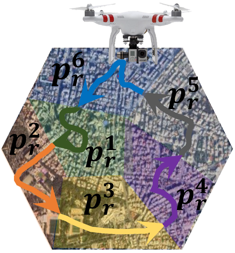
A single UAV is assigned to each region $r \in R$ and follows a flight path $p_{r}$ at height $h [m]$ . Because of speed constraints of the UAV, it may be infeasible for a UAV to monitor the whole of region $r$ in one time-step $k \in T$ . To circumvent this issue, we partition each path $p_{r}$ into sections of equal length, denoted as $p_{r}^{m}$ , where $m \in M_{r}$ is defined by the ordered set $M_{r} = {1, 2, . . ., M_{r}}$ , where M_r is the number of visiting areas for region r. As such, a UAV monitors a path section $p_{r}^{m}$ instead of the entire path $p_{r}$ during a single time-step $k \in T$ . The area monitored by the path section $p_{r}^{m}$ at time-step $k$ is known as a visiting area.

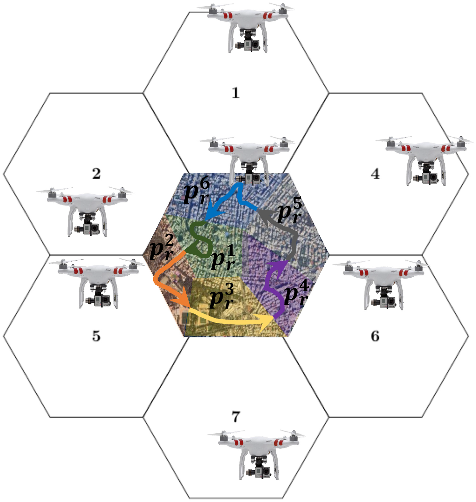
Figure 1 is a visual representation of a hexagonal region $r \in R$ divided into $M_{r} = 6$ UAV visiting areas, each denoted with a different color. Without loss of generality, we represent each region $r \in R$ as a hexagon as it is the largest polygon that can be tiled without leaving any empty space, making it useful for visually representing homogeneous regions of a traffic network ( 25 ). The UAV assigned to the hexagonal region in Figure 1 monitors a single visiting area over a discrete time-step, transitioning to the next visiting area along path $p_{r}$ with each subsequent time-step. For example, visiting areas 1 and 2 (green and orange visiting areas) in Figure 1 are observed by the UAV at time-steps {1,7,13,…} and {2,8,14,…}, respectively. As such, the UAV in Figure 1 completes one full cycle of path $p_{r}$ every six time-steps.

Figure 1.

A homogeneous hexagonal urban region divided into six visiting areas with a pre-determined unmanned aerial vehicle flight path.

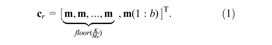
Let $m = [1, 2 . . ., M_{r}]$ be a vector identical to the ordered set $M_{r}$ and let the constant $b = mod (K, M_{r})$ . We define a vector $c_{r}$ as a column vector that maps every time-step $k \in T$ to visiting area $m \in M_{r}$ inhabited by a UAV for every region $r \in R$ :

c_{r} = [\underset{f l o o r (\frac{K}{M_{r}})}{\underset{︸}{\begin{matrix} m, m,..., m \end{matrix}}} \begin{matrix} , m (1 : b) \end{matrix}]^{T} .

(1)

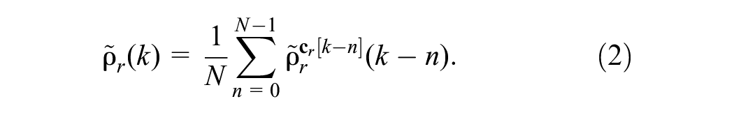
The UAVs have the ability to measure the visiting area regional density, ${\tilde{ρ}}_{r}^{m} (k)$ (veh/km) for a given visiting area $m \in M_{r}$ for region $r \in R$ and time-step $k \in T$ , subject to Gaussian noise. Each visiting area $m \in M_{r}$ differs in topology and has slight variations in vehicle density and mean speed with other visiting areas $m \in M_{r}$ . As such, we cannot make the assumption that ${\tilde{ρ}}_{r}^{m} (k) = {\tilde{ρ}}_{r} (k)$ , where ${\tilde{ρ}}_{r} (k)$ is the measured vehicle density.

To circumvent this problem, we express ${\tilde{ρ}}_{r} (k)$ as a moving average of the measurements ${\tilde{ρ}}_{r}^{m}$ :

{\tilde{ρ}}_{r} (k) = \frac{1}{N} \sum_{n = 0}^{N - 1} {\tilde{ρ}}_{r}^{c_{r} [k - n]} (k - n).

(2)

The summations occur over a moving window of $N$ time-steps, beginning at time-step $k - N + 1$ up until the current time-step $k$ . The visiting areas $m \in M_{r}$ are related to the current time-step $k$ by the vector $c_{r}$ at element $k$ , denoted as $c_{r} [k]$ .

We assume that UAVs have a clear, unobstructed view of each visiting area $m \in M_{r}, \forall k \in T$ . Moreover, it is assumed that once the UAV’s battery is approaching empty, the UAV can land at pre-designated spots and have its battery swapped with a fully charged one, as was done in ( 20 ). The time taken to swap out a battery and resume flight is considered negligible, and therefore it is not factored into our simulation results. Although modern UAVs have flight times of roughly 30 min in ideal conditions, it is possible that UAVs with flight times of a few hours may be commercialized in the future ( 26 ), such that UAV battery swapping may become less frequent.

The proposed UAV architecture utilizes the maneuverability that multi-rotor UAVs have over other mobile sensors. As UAVs are airborne, they can monitor far more spatial traffic information than mobile sensors, such as probe vehicles and GPS-enabled phones. Moreover, because they are not constrained by roads and vehicle congestion, they can traverse larger distances over a shorter period of time compared to other mobile sensors. As such, ${\tilde{ρ}}_{r} (k)$ can be obtained by monitoring a succession of small visiting areas $m \in M_{r}$ and using a moving average of the measurements ${\tilde{ρ}}_{r}^{m} (k)$ . Since only one UAV is required per region $r \in R$ , the proposed UAV-based sensing architecture is far more cost effective than other mobile sensor-based methods, as fewer sensors are required and fewer personnel are needed to operate each sensor. Lastly, because of the availability of UAVs and UAV trained pilots, this architecture can be applied over any urban area, so long as the maximum height of the buildings in the urban area does not exceed $h$ , the flight height of the UAVs.

Regional Traffic Model

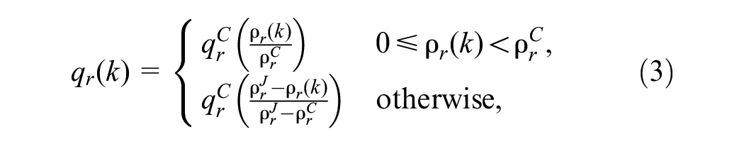
Let $q_{r} (k)$ (vehicles per hour [veh/h]) be the intended vehicle outflow at time-step $k \in T$ for region $r \in R$ , given as the product of the region density $ρ_{r} (k)$ [veh/km] and speed $u_{r} (k)$ [km/h] at time-step $k$ , that is, $q_{r} (k) = ρ_{r} (k) u_{r} (k)$ . The MFD expresses $q_{r} (k)$ as a piecewise function of $ρ_{r} (k)$ , given by the following:

q_{r} (k) = {\begin{matrix} q_{r}^{C} (\frac{ρ_{r} (k)}{ρ_{r}^{C}}) & 0 \leq ρ_{r} (k) < ρ_{r}^{C}, \\ q_{r}^{C} (\frac{ρ_{r}^{J} - ρ_{r} (k)}{ρ_{r}^{J} - ρ_{r}^{C}}) & otherwise, \end{matrix}

(3)

where $q_{r}^{C}$ is the maximum vehicle outflow, $ρ_{r}^{C}$ the critical density, and $ρ_{r}^{J}$ the jam density. Maximum vehicle outflow $q_{r}^{C}$ occurs when $ρ_{r} = ρ_{r}^{C}$ , while $q_{r} = 0$ occurs at the jam density $ρ_{r} = ρ_{r}^{J}$ for $r \in R$ . When the traffic density takes in values of $0 \leq ρ_{r} (k) < ρ_{r}^{C}$ the network operates under free-flow (uncongested) conditions, while if $ρ_{r}^{C} \leq ρ_{r} (k) \leq ρ_{r}^{J}$ the network operates under congestion. Note that when $ρ_{r} \leq ρ_{r}^{C}$ , the average speed of region $r \in R$ is the free-flow speed $u_{r}^{f} [km / h]$ $\forall r \in R$ .

Let $ρ_{rd} (k)$ be the density of vehicles in region $r \in R$ with final destination region $d \in D$ at time-step $k$ . Similarly, let $q_{rd} (k)$ be an intended vehicle transfer flow from region $r \in R$ to destination region $d \in D$ , such that $q_{rd} (k) = ρ_{rd} (k) u_{r} (k)$ . These are expressed by the following:

ρ_{r} (k) = \sum_{d \in D} ρ_{rd} (k),

(4)

q_{r} (k) = \sum_{d \in D} q_{rd} (k) .

(5)

Let $J_{r}^{-}$ be the set of regions that directly neighbor region $r \in R$ and let $J_{r}^{+}$ be the set of regions that directly neighbor region $r \in R$ but include region $r$ such that $J_{r}^{+} = J_{r}^{-} \cup {r}$ . The set $J_{r}$ is defined as follows:

J_{r} = {\begin{matrix} J_{r}^{+} & if r \in D, \\ J_{r}^{-} & if r \notin D . \end{matrix}

(6)

Note that vehicles entering and exiting region $r \in R$ can only do so via region $j$ , where $j \in J_{r}$ .

Let $ρ_{rjd} (k)$ be the density of vehicles in region $r \in R$ with final destination $d \in D$ through neighboring region $j \in J$ at time-step $k$ . Likewise, let $q_{rjd} (k)$ be the intended vehicle transfer flow from region $r \in R$ to destination region $d \in D$ through neighboring region $j \in J_{r}$ at time-step $k$ . Terms $ρ_{rd} (k), ρ_{rjd} (k), q_{rd} (k), q_{rjd} (k)$ are related by the following:

q_{rd} (k) = \sum_{j \in J_{r}} q_{rjd} (k),

(7)

ρ_{rd} (k) = \sum_{j \in J_{r}} ρ_{rjd} (k) .

(8)

Note that if $r = j = d$ , the vehicle is in its destination region $d \in D$ and will exit the traffic network and the vehicle exit flow $q_{ddd} (k)$ applies. In addition $q_{djd} (k) = 0$ where $j \in J_{r}^{-}$ , and therefore $q_{dd} (k) = q_{ddd} (k)$ .

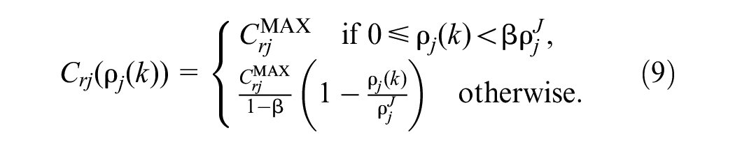
The interboundary flow capacity $C_{rj} (ρ_{j} (k)) [veh / h]$ determines the rate at which vehicles can enter a neighboring region $j \in J_{r}^{-}$ from $r \in R$ , and is a piecewise function of $ρ_{j} (k)$ with two pieces (i) a constant value $C_{rj}^{MAX}$ [veh/km] and (ii) a decreasing linear function of $ρ_{j} (k)$ :

C_{rj} (ρ_{j} (k)) = {\begin{matrix} C_{rj}^{MAX} if 0 \leq ρ_{j} (k) < β ρ_{j}^{J}, \\ \frac{C_{rj}^{MAX}}{1 - β} (1 - \frac{ρ_{j} (k)}{ρ_{j}^{J}}) otherwise . \end{matrix}

(9)

The term $C_{rj}^{MAX}$ [veh/h] is the maximum interboundary flow capacity from $r \in R$ to $j \in J$ and $0 < β < 1$ is a parameter that defines the point where interboundary capacity starts to decrease ( 27 ).

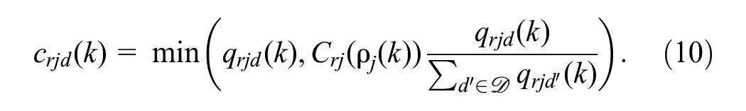
The actual vehicle transfer flow from $r \in R$ to destination $d \in D$ through neighboring region $j \in J_{r}$ is defined as follows:

c_{rjd} (k) = min (q_{rjd} (k), C_{rj} (ρ_{j} (k)) \frac{q_{rjd} (k)}{\sum_{d' \in D} q_{rjd'} (k)}) .

(10)

As shown above, $c_{rjd} (k)$ is the minimum of two terms: (i) an intended vehicle transfer flow $q_{rjd} (k)$ , from region $r \in R$ to the next neighboring region $j \in J_{r}$ and destination region $d \in D$ , and (ii) the interboundary flow capacity between regions $r \in R$ and $j \in J_{r}$ .

The term $c_{rj} (k)$ is expressed as a summation of $c_{rjd} (k)$ over the destination regions $d \in D$ :

c_{rj} (k) = \sum_{d \in D} c_{rjd} (k) .

(11)

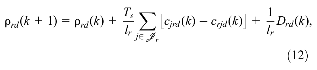
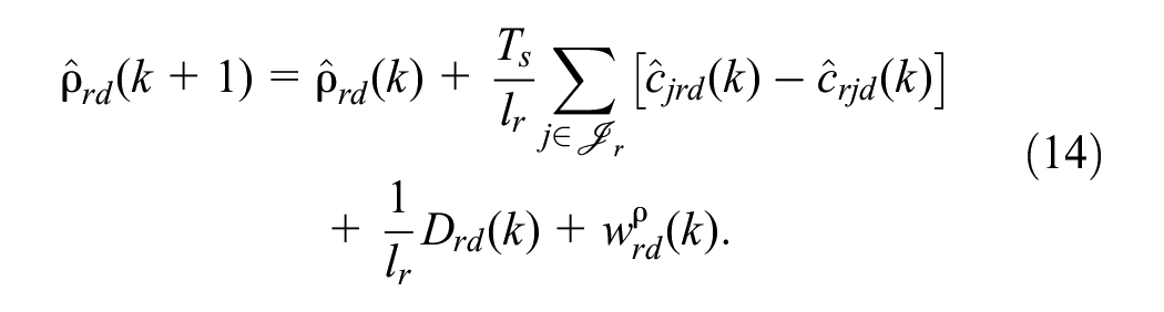
The traffic conservation equation computes $ρ_{rd} (k + 1)$ , and is expressed as follows:

ρ_{rd} (k + 1) = ρ_{rd} (k) + \frac{T_{s}}{l_{r}} \sum_{j \in J_{r}} [c_{jrd} (k) - c_{rjd} (k)] + \frac{1}{l_{r}} D_{rd} (k),

(12)

where $T_{s}$ is the simulation time-step, $D_{rd} (k)$ is the number of vehicles entering the network from region $r \in R$ during time-step $k \in T$ destined to region $d \in D$ , and $l_{r}$ [km] is the average road length of region $r \in R$ . Note that $l_{r}$ is chosen such that it satisfies the Courant–Friedrichs–Lewy condition ( 28 ), and therefore we have that $T_{s} \leq l_{r} \ u_{r}^{f}$ .

Problem Statement

The measured parameters ${\tilde{ρ}}_{r} (k)$ and ${\tilde{u}}_{r} (k)$ defined in the second section are subject to Gaussian measurement noise from the UAV and process noise, that is, the noise between the traffic model described in the third section and the actual vehicle dynamics in real urban areas. To minimize these errors, we develop a novel optimization problem which inputs the noisy measurements from the UAVs ${\tilde{ρ}}_{r} (k)$ , ${\tilde{u}}_{r} (k)$ and outputs estimated regional densities ${\hat{ρ}}_{r} (k),$ ${\hat{ρ}}_{rd} (k),$ $\forall k \in T,$ $\forall r \in R,$ $\forall d \in D$ . The aim is to achieve values of ${\hat{ρ}}_{r} (k),$ ${\hat{ρ}}_{rd} (k)$ that are as close as possible to the true regional densities $ρ_{r} (k)$ , $ρ_{rd} (k)$ .

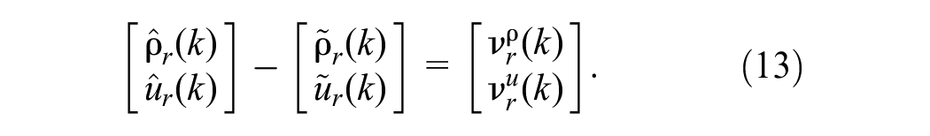
We define the estimation errors $ν_{r}^{ρ} (k),$ $ν_{r}^{u} (k)$ as the difference between ${\hat{ρ}}_{r} (k),$ ${\hat{u}}_{r} (k)$ and the measured regional parameters ${\tilde{ρ}}_{r} (k),$ ${\tilde{u}}_{r} (k),$ $\forall k \in T,$ $\forall r \in R$ :

[\begin{matrix} {\hat{ρ}}_{r} (k) \\ {\hat{u}}_{r} (k) \end{matrix}] - [\begin{matrix} {\tilde{ρ}}_{r} (k) \\ {\tilde{u}}_{r} (k) \end{matrix}] = [\begin{matrix} ν_{r}^{ρ} (k) \\ ν_{r}^{u} (k) \end{matrix}] .

(13)

The parameters $ν_{r}^{ρ} (k), ν_{r}^{u} (k)$ follow a normal distribution such that $ν_{r}^{ρ} (k) ~ N (μ_{ρ}, σ_{ρ}^{2})$ , $ν_{r}^{u} (k) ~ N (μ_{u}, σ_{u}^{2})$ , where $μ_{ρ} = μ_{u} = 0$ . Vector forms of these quantities are denoted as $\hat{ρ} (k)$ , $\tilde{ρ} (k)$ , $\hat{u} (k)$ , $\tilde{u} (k)$ , $ν^{ρ} (k)$ , $ν^{u} (k) \in R^{R \times 1}$ .

We define the estimated traffic conservation equation, given by the following:

\begin{matrix} {\hat{ρ}}_{rd} (k + 1) = & {\hat{ρ}}_{rd} (k) + \frac{T_{s}}{l_{r}} \sum_{j \in J_{r}} [{\hat{c}}_{jrd} (k) - {\hat{c}}_{rjd} (k)] \\ + \frac{1}{l_{r}} D_{rd} (k) + w_{rd}^{ρ} (k) . \end{matrix}

(14)

The above equation is identical to the traffic conservation equation (12) with the addition of the process error $w_{rd}^{ρ} (k)$ , where $w_{rd}^{ρ} (k) ~ N (μ_{w}, σ_{w}^{2})$ , $μ_{w} = 0$ .

We formulate the problem of finding the best estimates of ${\hat{ρ}}_{r} (k), {\hat{ρ}}_{rd} (k)$ as a least squares minimization problem. We employ a moving horizon window of fixed length $W$ looking into the past, such that $K_{k - W + 1}^{k} = {k - W + 1, k - W + 2, . . ., k}$ denotes the time window considered at time-step $k$ .

The minimization routine aims to find an optimal solution that minimizes the estimation errors $ν_{r}^{ρ} (k), ν_{r}^{u} (k)$ and process errors $w_{rd}^{ρ} (k)$ for the whole of the moving horizon window. The estimation and process errors $ν_{r}^{ρ} (k), ν_{r}^{u} (k), w_{rd}^{ρ} (k)$ for time-step $k$ are expressed as a single column vector

e_{k} = [ν_{r}^{ρ} (k), ν_{r}^{u} (k), w_{rd}^{ρ} (k)]^{T},

(15)

where $\forall r \in R, \forall d \in D, \forall k \in K_{k - W + 1}^{k}$ .

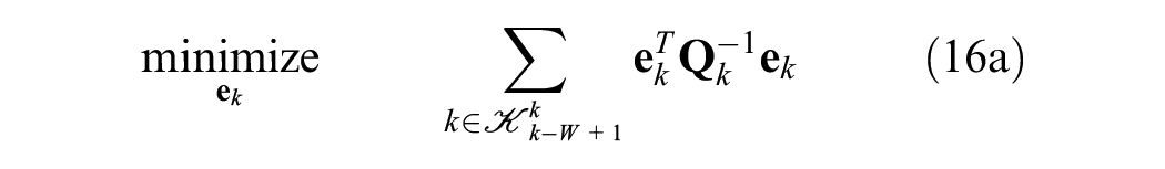
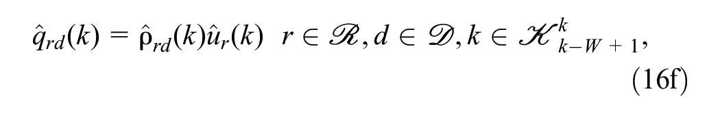
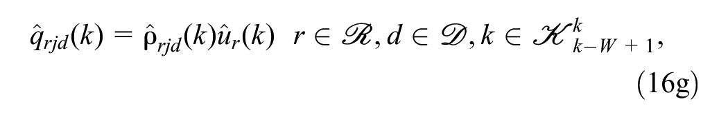
The optimization problem, referred to as P1, is defined by the following:

\underset{e_{k}}{minimize} \sum_{k \in K_{k - W + 1}^{k}} e_{k}^{T} Q_{k}^{- 1} e_{k}

(16a)

subject to traffic dynamics: Equations 3−11 and 13−15:

0 \leq {\hat{ρ}}_{r} (k) \leq ρ_{r}^{J} r \in R, k \in K_{k - W + 1}^{k},

(16b)

0 \leq {\hat{q}}_{r} (k) \leq q_{r}^{C} r \in R, k \in K_{k - W + 1}^{k},

(16c)

0 \leq {\hat{u}}_{r} (k) \leq u_{r}^{f} r \in R, k \in K_{k - W + 1}^{k},

(16d)

{\hat{q}}_{r} (k) = {\hat{ρ}}_{r} (k) {\hat{u}}_{r} (k) r \in R, k \in K_{k - W + 1}^{k},

(16e)

{\hat{q}}_{rd} (k) = {\hat{ρ}}_{rd} (k) {\hat{u}}_{r} (k) r \in R, d \in D, k \in K_{k - W + 1}^{k},

(16f)

{\hat{q}}_{rjd} (k) = {\hat{ρ}}_{rjd} (k) {\hat{u}}_{r} (k) r \in R, d \in D, k \in K_{k - W + 1}^{k},

(16g)

Variables $: {\hat{ρ}}_{rjd} (k), {\hat{q}}_{rjd} (k), {\hat{c}}_{rjd} (k), {\hat{u}}_{r} (k), ν_{r}^{ρ} (k), ν_{r}^{u} (k), w_{rd}^{ρ} (k) .$

Equation (16a) is the objective function to be minimized, given as the sum of squared errors defined by Equation (15), where the matrix $Q_{k}$ is the covariance matrix of the error vector $e_{k}$ . The errors are minimized over the entire moving horizon window $k \in K_{k - W + 1}^{k}$ . Constraints (3)–(11) and (13)–(15) are the traffic dynamics, while inequalities (16b)–(16d) impose physical constraints on the variables ${\hat{ρ}}_{r} (k), {\hat{q}}_{r} (k), {\hat{u}}_{r} (k)$ and (16e) and (16f) compute ${\hat{q}}_{r} (k)$ and ${\hat{q}}_{rd} (k)$ .

Note that P1 is non-convex and therefore nonlinear because of constraints (3), (9), (10), (16e), (16f). For the problem to converge to a global minimum, the constraints must be linearized such that the problem becomes convex.

Solution Approach

In this section, we develop a solution approach to problem P1 under free-flow conditions, that is, considering that $ρ_{r} (k) \leq min (ρ_{r}^{C}, β ρ_{r}^{J}), \forall r \in R, k \in K_{1}^{K}$ . We consider TSE in free-flow conditions as some traffic control strategies primarily focus on maintaining free-flow conditions to maximize traffic throughput ( 27 , 29 –32). Such strategies are employed before the traffic network reaches a congested state and therefore require accurate regional density values $ρ_{r}$ in real-time to be effective. Therefore, we limit the focus of our study to free-flow conditions only.

Under free-flow conditions, it is true that $u_{r} (k) = u_{r}^{f}$ such that the MFD relationship (3) is simplified to the following:

q_{r} (k) = ρ_{r} (k) u_{r}^{f} .

(17)

In a similar way, the nonlinear constraints $q_{rd} (k) = ρ_{rd} (k) u_{r} (k)$ and $q_{rjd} (k) = ρ_{rjd} (k) u_{r} (k)$ are changed into linear constraints:

q_{rd} (k) = ρ_{rd} (k) u_{r}^{f},

(18)

q_{rjd} (k) = ρ_{rjd} (k) u_{r}^{f} .

(19)

Under free-flow conditions it is also true that $C_{rj} (ρ_{j} (k)) = C_{rj}^{MAX}$ . Therefore, Equation (10) can be simplified into the following inequality constraints:

c_{rjd} (k) = q_{rjd} (k),

(20)

\sum_{d \in D} c_{rjd} (k) \leq C_{rj}^{MAX} .

(21)

Following the re-formulations of the nonlinear constraints, the linear minimization problem P2 is defined by the following:

\underset{e_{k}}{minimize} \sum_{k \in K_{k - W + 1}^{k}} e_{k}^{T} Q_{k}^{- 1} e_{k}

(22a)

subject to traffic dynamics (4)–(8), (11), (13)–(15), (17)–(21)

0 \leq {\hat{ρ}}_{r} (k) \leq ρ_{r}^{C} r \in R, k \in K_{k - W + 1}^{k},

(22b)

0 \leq {\hat{q}}_{r} (k) \leq q_{r}^{C} r \in R, k \in K_{k - W + 1}^{k},

(22c)

Variables $: {\hat{ρ}}_{rjd} (k), {\hat{q}}_{rjd} (k), {\hat{c}}_{rjd} (k), ν_{r}^{ρ} (k), ν_{r}^{u} (k), w_{rd}^{ρ} (k) .$

Problem P2 is identical to P1, but with all nonlinear constraints relaxed to form a completely linear (therefore convex) optimization problem. We solve P2 at every time-step $k \in T$ to obtain the best estimates of ${\hat{ρ}}_{r} (k), {\hat{ρ}}_{rd} (k)$ .

Simulation Results

We assume an urban traffic network, which we split into $R = 7$ homogeneous regions, where each region $r \in R$ can be both an origin and destination region, and therefore $R \equiv O \equiv D$ . The length of each region $r \in {1, 2 . . ., 7}$ is set to $[2, 4, 3, 2, 3, 5, 4]$ km, respectively. We assume also that each region is split into $M_{r} = 6$ visiting areas, where $r \in R$ . Figure 2 shows a visual representation of the traffic network, where visiting areas $m \in M_{r}$ are shown for region $r = 3$ only. We assume: $ρ_{r}^{C} = 30 veh / km$ , $ρ_{r}^{J} = 130 veh / km$ , $q_{r}^{C} = 1500$ [veh/h], $C_{rj}^{MAX} = 1500$ [veh/h], $u_{r}^{f} = 50 km / h$ , $β = \frac{ρ_{r}^{C}}{ρ_{r}^{J}}$ , and $T_{s} =$ 1/60 hours.

Figure 2.

Urban traffic network split into seven hexagonal regions where an unmanned aerial vehicle (UAV) is monitoring each region. Region $r = 3$ (center) shows the six visiting areas that contain the pre-determined flight path of the UAV.

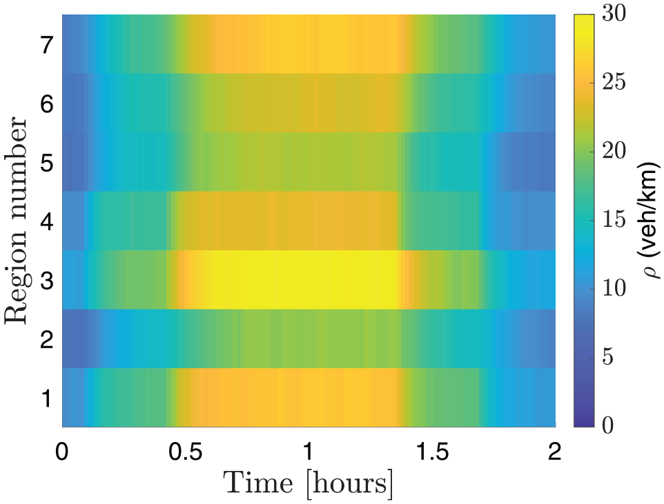
The simulation represents a medium demand, free-flow scenario where peak densities are close to the critical density $ρ_{r}^{C} = 30 veh / km$ and the total simulation runtime is $K = 120$ time-steps, therefore $T = 2$ h. The vehicle demand for the traffic network is dictated by the origin–destination matrix $D$ . The demand increases linearly up until time-step $k = 40$ , held constant until time-step $k = 70$ , and linearly decreases until time-step $k = 120$ , the end of the simulation. As shown in Figure 3, the peak density for all regions occurs around the 1 h mark. For simulations where $ρ_{r} (k) \leq ρ_{r}^{C}, \forall r \in R, \forall k \in T$ , Equations (17)–(19) and (20) are changed from inequalities to equalities, as all of the intended vehicle outflow $q_{r} (k)$ is modeled by the free-flow section of the MFD.

Figure 3.

Space–time graph of the regional density $ρ_{r} (k)$ because of traffic demand, averaged over 10 simulations.

Two UAV sensing architectures were simulated. The first is the architecture proposed in the second section, with the moving average window set to $N = 6$ , and is therefore known as UAV architecture 1. The second UAV-based sensing architecture places a single UAV in every visiting area $m$ and each UAV stays along the path $p_{r}^{m}$ , rather than cycling across the whole path $p_{r}$ , and is known as UAV architecture 2. Evidently, UAV architecture 2 is more expensive and requires more processing power as it contains six times the number of UAVs compared to UAV architecture 1, but it is expected to be more accurate as $ρ_{r}^{m} (k)$ and $u_{r}^{m} (k)$ are monitored and updated for $\forall r \in R$ , $\forall m \in M$ , $\forall k \in T$ . The UAV flight height $h$ is set to 150 m to provide a large field of view without compromising the effectiveness of the traffic monitoring algorithm ( 33 ). For both simulations, the length of the moving horizon window $W$ is set to 20 time-steps.

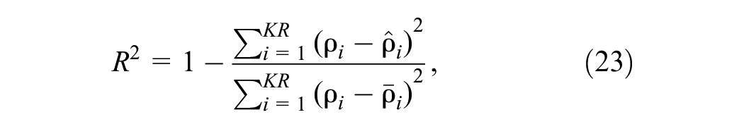
The process and measurement errors at every time-step $k \in T$ are minimized over the moving horizon window W using optimization problem P2. For the solution of problem P2 the barrier method of Gurobi was used; the optimization problem is solved in under 2 s in about 30 iterations. The simulation experiment is run 10 times with a demand scenario that yields the regional density shown in Figure 3, and the estimated values of ${\hat{ρ}}_{r} (k)$ and ${\hat{ρ}}_{rd} (k)$ are averaged $\forall k \in T$ for the 10 different runs of the experiment. We calculate $R^{2}$ as:

R^{2} = 1 - \frac{{\sum_{i = 1}^{KR} (ρ_{i} - {\hat{ρ}}_{i})}^{2}}{{\sum_{i = 1}^{KR} (ρ_{i} - {\bar{ρ}}_{i})}^{2}},

(23)

and the root mean square error (RMSE), which measures the magnitude of errors between the true values $ρ_{i}$ and the estimated ${\hat{ρ}}_{i}$ , as:

RMSE = \sqrt{\frac{{\sum_{i = 1}^{KR} (ρ_{i} - {\hat{ρ}}_{i})}^{2}}{KR}} .

(24)

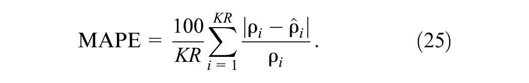
In Equations (23)–(25), $ρ_{i} = ρ_{r} (k)$ , ${\hat{ρ}}_{i} = {\hat{ρ}}_{r} (k)$ , and ${\bar{ρ}}_{i} = {\bar{ρ}}_{r} (k)$ , where ${\bar{ρ}}_{r} (k)$ is the average value of $ρ_{r} (k), \forall r \in R$ , $\forall k \in T$ , for calculations involving $ρ_{r} (k)$ . The mean average percentage error (MAPE) measures the average magnitude of error between the true values $ρ_{i}$ and estimated ${\hat{ρ}}_{i}$ as a percentage, given by the following:

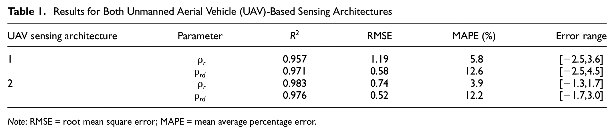
MAPE = \frac{100}{KR} \sum_{i = 1}^{KR} \frac{| ρ_{i} - {\hat{ρ}}_{i} |}{ρ_{i}} .

(25)

Note that for MAPE calculations, $ρ_{i}$ and ${\hat{ρ}}_{i}$ values less than 1 veh/km were not included as small values that differ slightly can lead to high MAPE errors. The results for both UAV architectures are shown in Table 1.

Table 1.

Results for Both Unmanned Aerial Vehicle (UAV)-Based Sensing Architectures

UAV sensing architecture	Parameter	$R^{2}$	RMSE	MAPE (%)	Error range
1	$ρ_{r}$	0.957	1.19	5.8	[−2.5,3.6]
	$ρ_{rd}$	0.971	0.58	12.6	[−2.5,4.5]
2	$ρ_{r}$	0.983	0.74	3.9	[−1.3,1.7]
	$ρ_{rd}$	0.976	0.52	12.2	[−1.7,3.0]

Note: RMSE = root mean square error; MAPE = mean average percentage error.

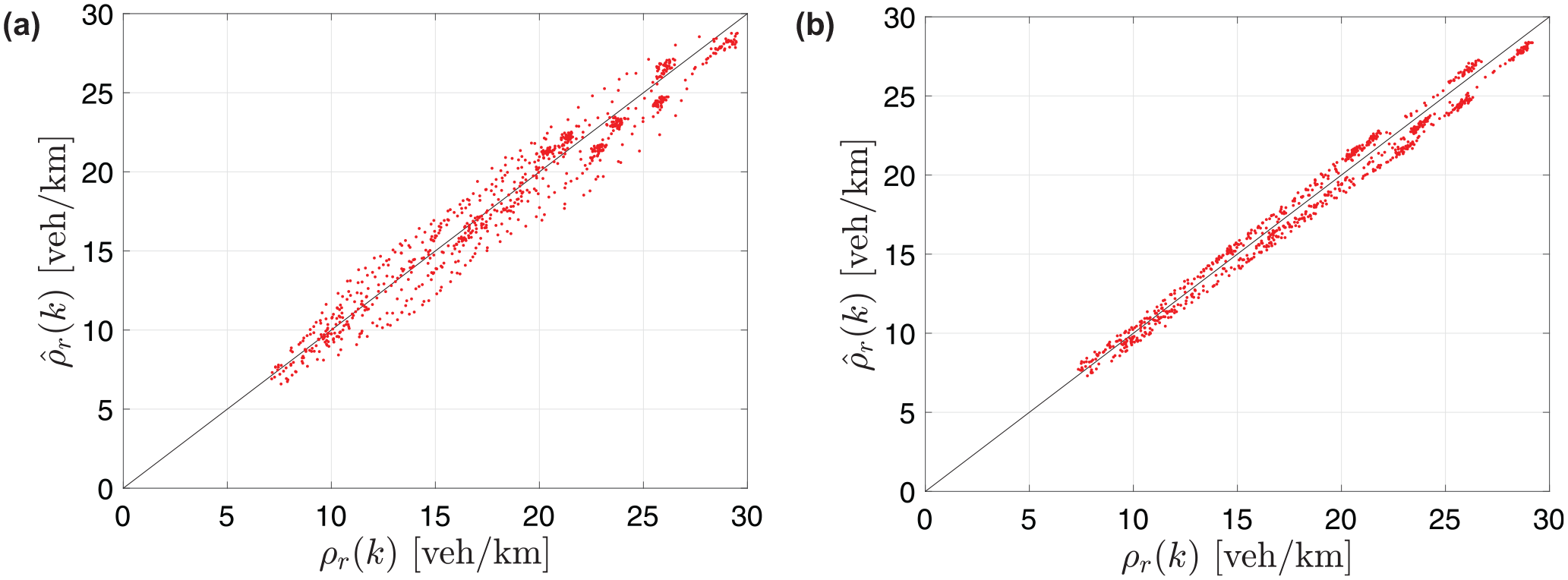
Figure 4a and 4b, plots the estimated regional density ${\hat{ρ}}_{r} (k)$ against the true density $ρ_{r} (k)$ from the simulation for UAV sensing architectures 1 and 2, respectively. The $R^{2}$ value for UAV architecture 1 is 0.957, while for UAV architecture 2 it is 0.983, a 2.7% increase. Both $R^{2}$ values are close to 1, indicating a strong correlation between ${\hat{ρ}}_{r} (k)$ and $ρ_{r} (k)$ . As expected, the $R^{2}$ for UAV architecture 2 is greater than that of UAV architecture 1, although the percentage difference is not particularly high. The high accuracy of the estimated parameters is also shown by the low RMSEs, which are 1.19 and 0.74 veh/km, respectively, for UAV architectures 1 and 2. The RMSE for UAV architecture 2 is 37.8% lower than that for UAV architecture 1, as the values of ${\hat{ρ}}_{r} (k)$ and $ρ_{r} (k)$ have a lower variance, which can be verified visually by inspecting Figure 4a and 4 b. The MAPE also suggests that UAV architecture 2 is more accurate than UAV architecture 1, with MAPE values of 3.9% and 5.8%, respectively. The MAPE of UAV architecture 2 is 32.8% lower than that of UAV architecture 1, which is similar to the difference in RMSE values between the two architectures.

Figure 4.

Plot of averaged ${\hat{ρ}}_{r} (k)$ versus $ρ_{r} (k)$ for both unmanned aerial vehicle (UAV)-based sensing architectures: (a) UAV architecture 1 and (b) UAV architecture 2.

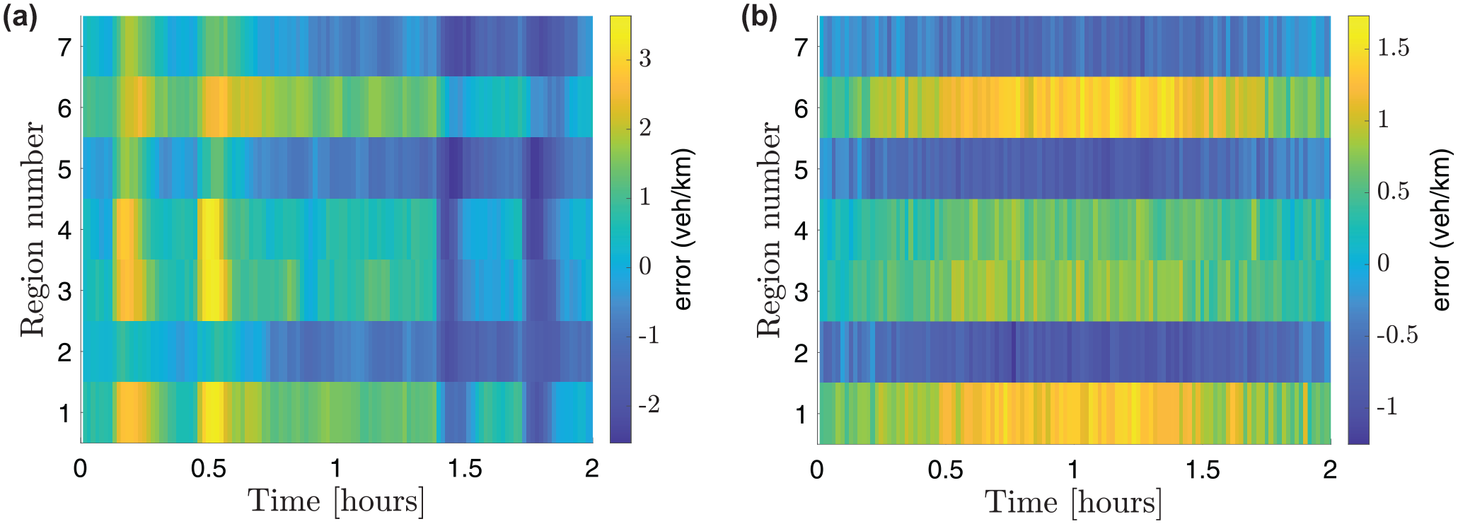
Figure 5a and 5b, plots the difference between $ρ_{r}$ and ${\hat{ρ}}_{r}$ as a colormap. The error range of estimated densities ${\hat{ρ}}_{r} (k)$ for UAV architecture 1 is [−2.5,3.6] veh/km, whereas for UAV architecture 2 it is [−1.3,1.7] veh/km. The ranges for UAV architecture 1 are greater, which is expected given that the RMSE is greater and the $R^{2}$ lower for UAV architecture 1 compared to UAV architecture 2. For UAV architecture 1, the maximum deviations occur around the 0.25, 0.5, 1.5 and 1.75 h mark, as shown in Figure 5a. This can be explained by the traffic demand increasing sharply at times 0.25 and 0.5 h and then decreasing at times 1.5 and 1.75 h. Because of the nature of the moving average, the estimator does not react immediately to the changes in demand, and therefore it underestimates ${\hat{ρ}}_{r}$ before the 1 h mark, and overestimates after. Note that this is not the case with UAV architecture 2, which updates ${\tilde{ρ}}_{r}^{m} (k)$ at every time-step $\forall k \in K$ , $\forall m \in M,$ $\forall r \in R$ . Figure 5b indicates that the maximum deviations occur around the 1 h mark, where traffic density is at its highest.

Figure 5.

Space–time graph of $ρ_{r} (k)$ – ${\hat{ρ}}_{r} (k)$ for both unmanned aerial vehicle (UAV)-based sensing architectures: (a) UAV architecture 1 and (b) UAV architecture 2.

Values for $ρ_{rd} (k)$ can be estimated but not measured, as it is impossible for a UAV to identify the destination region $d \in D$ for each vehicle in the traffic network. Having an accurate estimate ${\hat{ρ}}_{rd} (k)$ is useful for applying effective control laws to minimize congestion in the road network, although this is outside the scope of this work.

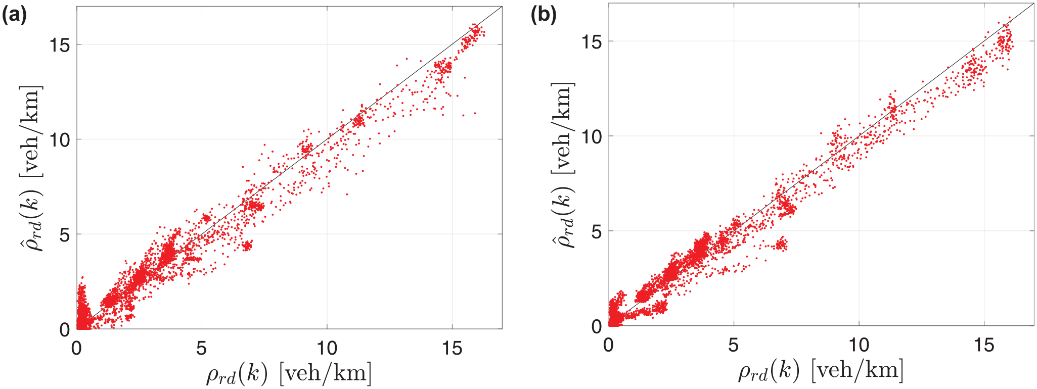
Figure 6a and 6b, plots ${\hat{ρ}}_{rd} (k)$ against $ρ_{rd} (k)$ for UAV sensing architectures 1 and 2, respectively. As was the case with the $ρ_{r} (k)$ values, the $R^{2}$ values are both close to 1 at 0.971 and 0.976, respectively, for UAV sensing architectures 1 and 2, indicating a very strong positive correlation. Moreover, the percentage difference between UAV sensing architectures 1 and 2 is very low at 0.5%, and is therefore considered negligible. This is because the majority of $ρ_{rd} (k)$ values are much lower than the $ρ_{r} (k)$ values, and therefore the deviations are not so great, so ${\hat{ρ}}_{rd} (k) \approx ρ_{rd} (k)$ when $ρ_{rd} (k)$ is low. This is shown in Figure 6a and 6b, where the majority of points lie close to the ${\hat{ρ}}_{rd} (k) = ρ_{rd} (k)$ line. Moreover, this explains the similarity of the RMSEs, which are 0.58 veh/km for UAV sensing architecture 1 and 0.52 for UAV sensing architecture 2, a 10.3% decrease. The MAPEs are relatively high for UAV sensing architectures 1 and 2 at 12.6% and 12.2%, respectively. The reason for this is that unlike $ρ_{r}$ , $ρ_{rd}$ values cannot be measured by the UAV and therefore estimations are less accurate. Also, the values of $ρ_{rd}$ are generally quite low, so small deviations result in a large MAPE. As expected, UAV architecture 2 is more accurate than UAV architecture 1 at estimating $ρ_{rd} (k)$ , although it is only 3.2% more accurate. As expected, the error range between ${\hat{ρ}}_{rd} (k)$ and $ρ_{rd} (k)$ is greater for UAV sensing architecture 1 than that for UAV sensing architecture 2, with errors ranges of [−2.5,4.5] and [−1.7,3.0] veh/km, respectively.

Figure 6.

Plot of averaged ${\hat{ρ}}_{rd} (k)$ versus $ρ_{rd} (k)$ for both unmanned aerial vehicle (UAV)-based sensing architectures: (a) UAV architecture 1 and (b) UAV architecture 2.

Overall, UAV sensing architecture 2 produced higher $R^{2}$ values and lower RMSE, MAPE, and deviations compared to UAV sensing architecture 1, as ${\tilde{ρ}}_{r}^{m} (k)$ was updated for $\forall k \in T$ , $\forall m \in M,$ $\forall r \in R$ . In contrast, only one ${\tilde{ρ}}_{r}^{m} (k)$ was updated for $\forall k \in T$ , $\forall r \in R$ for UAV sensing architecture 1, as there is only one UAV per region $r$ instead of one UAV per visiting area $m$ . Despite this, the difference in $R^{2}$ values are very small if not negligible for ${\hat{ρ}}_{r} (k)$ and ${\hat{ρ}}_{rd} (k)$ . The RMSE is 37.8% lower for ${\hat{ρ}}_{r} (k)$ between UAV sensing architectures 1 and 2 and 10.3% lower for ${\hat{ρ}}_{rd} (k)$ . Similarly, the MAPE is 32.8% lower for ${\hat{ρ}}_{r} (k)$ between UAV sensing architectures 1 and 2 and 3.2% lower for ${\hat{ρ}}_{rd} (k)$ . Given that UAV sensing architecture 2 requires six times more UAVs than UAV sensing architecture 1, this is considered a worthwhile trade-off, considering that all RMSEs are low and do not exceed 1.2 veh/km for any of the parameters. We have shown therefore through our simulations that our proposed UAV sensing architecture can obtain very respectable results while drastically reducing the number of UAVs and computational power needed by assigning one UAV per region $r$ instead of one UAV per visiting area $m$ .

Conclusions and Future Work

This work proposes a novel optimization framework that yields accurate density and mean speed estimations of an urban traffic network in real-time through the use of real-time UAV data. Our proposed UAV architecture splits the traffic network into homogeneous regions where each region is further split into smaller visiting areas. The UAVs follow a pre-determined, cyclical flight path above each traffic region, observing a visiting area at each time-step. Noisy measurements of density and mean speed are obtained at every time-step for the visiting area being observed. Using these measurements as inputs, estimates for regional density, regional mean speed, and regional densities with known destinations are obtained in real-time through a quadratic program solution approach that minimizes estimation and process errors over a moving horizon with a moving average of measurements.

Our proposed UAV-based sensing architecture was compared to a benchmark architecture where each visiting area in the traffic network is constantly monitored by a UAV, that is, full information of the traffic network is available for the benchmark architecture. Compared to this benchmark architecture, the proposed UAV sensing architecture produces high-quality estimations of regional density and regional density with known destinations assuming a free-flow traffic scenario, even though the proposed architecture utilizes six times less information obtained from the UAVs. We therefore conclude that full network TSE can be achieved using noisy UAV measurements from small parts of the traffic network under free-flow conditions. These findings highlight the potential for UAV-based TSE as an accurate and affordable alternative to other sensing approaches for traffic monitoring and TSE, such as stationary or other mobile sensors.

Future research work includes a variety of vehicle demand scenarios (light/heavy congestion), alternative UAV architectures and optimization frameworks, and additional measurements from UAVs (such as the transfer flows between regions) to increase estimation accuracy.

Supplemental Material

sj-pdf-1-trr-10.1177_03611981231213079 – Supplemental material for Real-Time Unmanned Aerial Vehicle-Based Traffic State Estimation for Multi-Regional Traffic Networks

Supplemental material, sj-pdf-1-trr-10.1177_03611981231213079 for Real-Time Unmanned Aerial Vehicle-Based Traffic State Estimation for Multi-Regional Traffic Networks by Kyriacos Theocharides, Charalambos Menelaou, Yiolanda Englezou and Stelios Timotheou in Transportation Research Record

Footnotes

Author Contributions

The authors confirm contribution to the paper as follows: study conception and design: K. Theocharides, C. Menelaou, Y. Englezou, S. Timotheou; data collection: K. Theocharides; analysis and interpretation of results: K. Theocharides, C. Menelaou, Y. Englezou; draft manuscript preparation: K. Theocharides, C. Menelaou, Y. Englezou, S. Timotheou. All authors reviewed the results and approved the final version of the manuscript.

Declaration of Conflicting Interests

The author(s) declared no potential conflicts of interest with respect to the research, authorship, and/or publication of this article.

Funding

The author(s) disclosed receipt of the following financial support for the research, authorship, and/or publication of this article: This work is supported by the European Union (i. ERC, URANUS, No. 101088124, ii. Horizon 2020 Teaming, KIOS CoE, No. 739551 and iii. Marie Sklodowska-Curie IF project: BITS, No. 101003435), and the Government of the Republic of Cyprus through the Deputy Ministry of Research, Innovation, and Digital Strategy. Views and opinions expressed are those of the author(s) only and do not necessarily reflect those of the European Union or the European Research Council Executive Agency. Neither the European Union nor the granting authority can be held responsible for them.

ORCID iDs

Kyriacos Theocharides

Charalambos Menelaou

Yiolanda Englezou

Stelios Timotheou

Supplemental Material

Supplemental material for this article is available online.

References

Seo

Bayen

A. M.

Kusakabe

Asakura

Traffic State Estimation on Highway: A Comprehensive Survey. Annual Reviews in Control, Vol. 43, 2017, pp. 128–151.

Munoz

Sun

Horowitz

Alvarez

Traffic Density Estimation with the Cell Transmission Model. Proceedings of the 2003 American Control Conference, Vol. 5, 2003, pp. 3750–3755.

Coifman

Estimating travel times and vehicle trajectories on freeways using dual loop detectors. Transportation Research Part A: Policy and Practice, Vol. 36, 2002, pp. 351–364.

Schoepflin

Dailey

Dynamic Camera Calibration of Roadside Traffic Management Cameras for Vehicle Speed Estimation. IEEE Transactions on Intelligent Transportation Systems, Vol. 4, No. 2, 2003, pp. 90–98.

Wang

Papageorgiou

Real-Time Freeway Traffic State Estimation Based on Extended Kalman Filter: A General Approach. Transportation Research Part B: Methodological, Vol. 39, 2005, pp. 141–167.

Sobie

Life Cycle Cost Analysis of Vehicle Detection Technologies and Their Impact on Adaptive Traffic Control Systems. Doctoral dissertation. Northern Arizona University, 2016.

Kong

Q.-J.

Chen

Liu

An Approach to Urban Traffic State Estimation by Fusing Multisource Information. IEEE Transactions on Intelligent Transportation Systems, Vol. 10, 2009, pp. 499–511.

Nantes

Ngoduy

Bhaskar

Miska

Chung

Real-Time Traffic State Estimation in Urban Corridors from Heterogeneous Data. Transportation Research Part C: Emerging Technologies, Vol. 66, 2016, pp. 99–118.

Kong

Q.-J.

Zhao

Wei

Liu

Efficient Traffic State Estimation for Large-Scale Urban Road Networks. IEEE Transactions on Intelligent Transportation Systems, Vol. 14, 2013, pp. 398–407.

10.

Herrera

J. C.

Work

D. B.

Herring

Ban

X. J.

Jacobson

Bayen

A. M.

Evaluation of Traffic Data Obtained via GPS-Enabled Mobile Phones: The Mobile Century Field Experiment. Transportation Research Part C: Emerging Technologies, Vol. 18, 2010, pp. 568–583.

11.

Butilă

E. V.

Boboc

R. G.

Urban Traffic Monitoring and Analysis Using Unmanned Aerial Vehicles (UAVs): A Systematic Literature Review. Remote Sensing, Vol. 14, No. 3, 2022, p. 620.

12.

Kyrkou

Timotheou

Kolios

Theocharides

Panayiotou

Drones: Augmenting Our Quality of Life. IEEE Potentials, Vol. 38, 2019, pp. 30–36.

13.

Kim

Ash

Cui

Wang

Real-Time Bidirectional Traffic Flow Parameter Estimation from Aerial Videos. IEEE Transactions on Intelligent Transportation Systems, Vol. 18, 2017, pp. 890–901.

14.

Tang

Pan

Wang

Real-Time Traffic Flow Parameter Estimation from UAV Video Based on Ensemble Classifier and Optical Flow. IEEE Transactions on Intelligent Transportation Systems, Vol. 20, 2019, pp. 54–64.

15.

Wang

Simeonova

Shahbazi

Orientation-and Scale-Invariant Multi-Vehicle Detection and Tracking from Unmanned Aerial Videos. Remote Sensing, Vol. 11, No. 18, 2019, p. 2155.

16.

Liu

Tang

Real-Time Object Detection in UAV Vision Based on Neural Processing Units. Proceedings of the IEEE 6th Information Technology and Mechatronics Engineering Conference (ITOEC), Vol. 6, 2022, pp. 1951–1955.

17.

Arkhipov

D. I.

Kim

Talcott

C. L.

Regan

A. C.

McCann

J. A.

Venkatasubramanian

ADDSEN: Adaptive Data Processing and Dissemination for Drone Swarms in Urban Sensing. IEEE Transactions on Computers, Vol. 66, 2017, pp. 183–198.

18.

Garcia-Aunon

Roldán

J. J.

Barrientos

Monitoring Traffic in Future Cities with Aerial Swarms: Developing and Optimizing a Behavior-Based Surveillance Algorithm. Cognitive Systems Research, Vol. 54, 2019, pp. 273–286.

19.

Elloumi

Dhaou

Escrig

Idoudi

Saidane

Monitoring Road Traffic with a UAV-Based System. Proc., IEEE Wireless Communications and Networking Conference, Barcelona, Spain, IEEE, New York, 2018, pp. 1–6.

20.

Barmpounakis

Geroliminis

On the New Era of Urban Traffic Monitoring with Massive Drone Data: The pNEUMA Large-Scale Field Experiment. Transportation Research Part C: Emerging Technologies, Vol. 111, 2020, pp. 50–71.

21.

Kyrkou

Timotheou

Kolios

Theocharides

Panayiotou

C. G.

Optimized Vision-Directed Deployment of UAVs for Rapid Traffic Monitoring. Proc., IEEE International Conference on Consumer Electronics (ICCE), Las Vegas, NV, IEEE, New York, 2018, pp. 1–6.

22.

Englezou

Timotheou

Panayiotou

Estimating the Origin-Destination Matrix Using Link Count Observations from Unmanned Aerial Vehicles. Proc., IEEE International Intelligent Transportation Systems Conference (ITSC), Indianapolis, IN, IEEE, New York, 2021, pp. 3539–3544.

23.

Englezou

Timotheou

Panayiotou

Probabilistic Traffic Density Estimation Using Measurements from Unmanned Aerial Vehicles. Proc., IEEE International Conference on Unmanned Aerial Systems (ICUAS), Dubrovnik, Croatia, IEEE, New York, 2022, pp. 1381–1388.

24.

Ramezani

Haddad

Geroliminis

Dynamics of Heterogeneity in Urban Networks: Aggregated Traffic Modeling and Hierarchical Control. Transportation Research Part B: Methodological, Vol. 74, 2015, pp. 1–19.

25.

Yildirimoglu

Ramezani

Geroliminis

Equilibrium Analysis and Route Guidance in Large-Scale Networks with MFD Dynamics. Transportation Research Procedia, Vol. 9, 2015, pp. 185–204.

26.

Wagter

C. D.

Remes

Smeur

van Tienen

Ruijsink

van Hecke

van der Horst

The NederDrone: A Hybrid Lift, Hybrid Energy Hydrogen UAV. International Journal of Hydrogen Energy, Vol. 46, 2021, pp. 16003–16018.

27.

Menelaou

Timotheou

Kolios

Panayiotou

C. G.

Joint Route Guidance and Demand Management for Real-Time Control of Multi-Regional Traffic Networks. IEEE Transactions on Intelligent Transportation Systems, Vol. 23, No. 7, 2022, pp. 8302–8315.

28.

Grandinetti

Canudas-de Wit

Garin

Distributed Optimal Traffic Lights Design for Large-Scale Urban Networks. IEEE Transactions on Control Systems Technology, Vol. 27, No. 3, 2019, pp. 950–963.

29.

Menelaou

Timotheou

Kolios

Panayiotou

C. G.

Polycarpou

M. M.

Minimizing Traffic Congestion Through Continuous-Time Route Reservations with Travel Time Predictions. IEEE Transactions on Intelligent Vehicles, Vol. 4, No. 1, 2019, pp. 141–153.

30.

Menelaou

Timotheou

Kolios

Panayiotou

C. G.

Improved Road Usage Through Congestion-Free Route Reservations. Transportation Research Record: Journal of the Transportation Research Board, 2017. 2621: 71–80.

31.

Menelaou

Kolios

Timotheou

Panayiotou

Polycarpou

Controlling Road Congestion via a Low-Complexity Route Reservation Approach. Transportation Research Part C: Emerging Technologies, Vol. 81, 2017, pp. 118–136.

32.

Kerner

B. S.

The Maximization of the Network Throughput Ensuring Free Flow Conditions in Traffic and Transportation Networks: Breakdown Minimization (BM) Principle Versus Wardrop’s Equilibria. The European Physical Journal B, Vol. 89, 2016, p. 199.

33.

Makrigiorgis

Kolios

Timotheou

Theocharides

Panayiotou

Extracting the Fundamental Diagram from Aerial Footage. Proc., IEEE 91st Vehicular Technology Conference, Antwerp, Belgium, IEEE, New York, 2020, pp. 1–5.

Supplementary Material

Please find the following supplemental material available below.

For Open Access articles published under a Creative Commons License, all supplemental material carries the same license as the article it is associated with.

For non-Open Access articles published, all supplemental material carries a non-exclusive license, and permission requests for re-use of supplemental material or any part of supplemental material shall be sent directly to the copyright owner as specified in the copyright notice associated with the article.

0.00 MB

0.20 MB