Sage Journals: Discover world-class research

Abstract

In this paper, we aim to answer two main questions in the context of multimodal travel and new modes of transportation, such as autonomous vehicles: firstly, as travelers gain the ability to readily compare modes side by side for each trip, will they become more willing to select the option that best meets their needs in the moment, or will they continue to prefer using a single mode for a whole tour? Secondly, we compare two approaches to estimating mode choice models in the context of a typical workday tour: one in which we enumerate each possible sequence of modes, and one in which we calculate the expected utility given all modes available for each trip separately, and sum over all trips in the tour. We find that the latter approach returns similar estimation results to the former, but is much faster and easier to compute, an advantage that would only grow with more mode alternatives or more trips in the tour. In addition, we discovered a substantial “mode inertia” in our sample: the utility of the mode used for the previous trip is significantly higher for the present trip. This finding indicates that respondents in our sample are more likely to stick with unimodal tours than multimodal ones.

Keywords

data and data science analysis modeling planning and analysis behavior analysis mode choices pattern (behavior choices etc.)preference survey data analysis

In a world with proliferating multimodal travel options and new modes including autonomous vehicles (AVs), it is increasingly important to understand how travelers make mode choices in the context of tours. As travelers gain the ability to readily compare modes side by side for each trip, will they become more willing to select the option that best meets their needs in the moment? Or will they continue to prefer using a single mode throughout a tour?

Answering this question is made more challenging by methodological limitations. When considering multiple mode options across multiple trips in a tour, there is a curse of dimensionality in which the choice set grows exponentially with the number of trips. However, considering each trip as an independent choice is not desirable either, because doing so disregards the motivation behind performing that trip and the interrelationships between consecutive trips. Although trip-based mode choice models may be appropriate in some cases, according to Ben-Akiva et al. ( 1 ), they lack “behavioral realism,” since individuals’ mode choices for different trips are usually not independent. Furthermore, travel surveys historically focus on collecting information about the primary mode of travel ( 2 ). Multimodal travel has been often neglected ( 3 ), although multimodal information is critical to comprehend the market demand for various modes beyond privately owned vehicles. However, a tour-based approach allows the analysis of multimodal travel behavior by anticipating the dependencies among the trips within the chain.

In this paper, we compare two approaches to estimating mode choice models in the context of a tour: one in which we enumerate each possible sequence of modes, and one in which we calculate the expected utility given all modes available for each trip separately, and sum over all trips in the tour. We find that the latter approach returns similar estimation results to the former, but is much faster and easier to compute, an advantage that would only grow with more mode alternatives or more trips in the tour.

We apply our model to test for evidence of “mode inertia,” the tendency for travelers to stick with a single mode in a tour. We find evidence of significant mode inertia when considering multimodal alternatives, and that this effect is stronger with some modes than with others.

The prior literature on tour-based mode choice behavior is not as common as the trip-based approach. As one of the earlier studies, Ben-Akiva et al. ( 1 ) explored the complexity of work tours in Boston, where they found that tour-based models match the process of making travel decisions more closely than trip-based approaches. They also highlighted that travel patterns vary dramatically across the population, and that simple trip-based models cannot capture the heterogeneous behavior of people and the variety of travel patterns. Capturing this heterogeneity and interdependence of choices is necessary when evaluating policies that aim to influence individuals’ behavior.

Tour-based mode choice models are often implemented as the components of activity-based models when decisions such as car ownership, residential location choice, or destination choice are also included in the analysis. Although previous studies used tour-based approaches to model mode choice behavior using various methods, the majority of them share some common traits, namely, (1) simplification in the definition and construction of tours and (2) the assumption of a “main” mode ( 4 ). Frank et al. ( 5 ) used a tour-based modeling framework to explore how travel time, cost, and land-use patterns affect mode choice and trip chaining behavior. Firstly, they identified the tour’s primary mode by identifying the mode that controls individuals’ travel planning. Following this, a mode choice model was developed for each type of tour (e.g., home-based work, home-based other, and work other work) using revealed preference data from a household travel survey conducted in the Puget Sound (Seattle, U.S.A.) Region. They found that travel time was the strongest predictor of mode choice, while urban form was the strongest predictor for the number of stops within a tour. Roorda et al. ( 6 ) also used a tour-based approach to incorporate minor travel modes (e.g., bicycling, drive/transit access commuter rail, drive access subway) into a simulation-based behaviorally realistic mode choice model. The authors reported limited success in modeling and correctly predicting some of the modes, such as drive access to subway, taxi, bicycle modes. Bastarianto et al. ( 7 ) studied the relationship between tour type and mode choices using logit models. However, their study did not explore multimodal tours, and it was focused on how travelers’ socio-economic characteristics influence their mode choices for different types of tours. Ho and Mulley ( 8 ) formulated a tour-based mode choice model contingent on the choice of joint tour patterns among household members. They adopted a nested logit framework for modeling individuals’ mode choice behavior by using the primary mode of travel. They assumed that if a car is used for the first trip of the tour, it must be used for the whole tour. Miller et al. ( 4 ) introduced a tour-based mode choice model framework that incorporates inter-personal interactions within a household. Their model allows variation in mode choices for different trips within a tour and assumes that respondents choose the “best” combination of modes available at the time of the trips. They assumed that the utility of choosing a combination of modes for the entire tour is equal to the sum of the utilities of the trips within the tour.

In the past few years, more studies have investigated latent variables, such as people’s perceptions and attitudes toward AVs and services, to better understand AV adoption motivations and barriers. For example, Haboucha et al. ( 13 ) explored the motivations of travelers to adopt AVs and modeled mode choices among regular cars, privately owned AVs, and shared AVs. They identified five latent variables using identifier questions from the prior literature and found three of them to be statistically significant in the mode choice model: (1) pro-AV attitudes; (2) enjoyment of driving; and (3) concern for the environment. As expected, their results showed that people who enjoy driving are more likely to use a regular car than an AV, and individuals with pro-AV attitudes are more inclined toward AVs. Concern for the environment was a more robust predictor for shared modes. Lavieri and Bhat ( 14 ) used a multivariate integrated choice and latent variable (ICLV) approach to explore which individuals would be willing to share an AV with strangers in the future. Their model included three latent variables: privacy-sensitivity, time-sensitivity, and interest in the productive use of travel time. They concluded that individuals who are more interested in using travel time productively are more likely to choose ride-hailing services. They also found that travelers dislike shared rides more because of delays than because of the presence of strangers. Wicki et al. ( 15 ) investigated the willingness to pay to use self-driving bus services. They incorporated technology-related attitudes to explore the tradeoffs between “technological skepticism” and the potential benefits of the service. They found that the technology acceptance latent variable is a strong predictor of self-driving bus usage. Rahimi et al. ( 16 ) analyzed people’s attitudes toward shared mobility options and AVs using a structural equations model. They identified 11 latent variables and explored their relationships with socio-economic characteristics and correlations between attitudes.

In this study, we adopted a tour-based approach to improve behavioral realism by capturing interdependencies between mode choices for trips in multimodal tours. Behavioral realism is particularly important in the context of automated vehicles and future mobility services to understand how travelers incorporate these modes in their travel routines, since they have no experience planning their travels using these modes. We compare two different approaches to estimating a tour-based mode choice model, and compare the results of the tour-based models to a trip-based mode choice model. We used a dataset collected through an interactive stated preference survey described in prior papers ( 9 , 10 ), and hypothesized two possible models of travelers’ decision processes: one in which they enumerate all possible mode sequence combinations (which we refer to as the full choice set approach), and one in which travelers make mode choices based on the expected utility across all modes in future trips (we refer to this as the approximation approach). We used an ICLV model to explicitly model how two latent constructs—perception of AV safety and car ownership importance—affect mode choices involving AVs and driverless ride-hailing services. In a previous study ( 10 ) using the same dataset, we found these two latent constructs have a statistically significant and meaningful effect on choosing AVs and driverless ride-hailing services. Therefore, we incorporated them to be consistent with the previous study and allow comparison of the models.

These models are developed more thoroughly in the Methods section of this paper. Based on these two decision processes, we formulated and estimated four models. We will discuss the results and findings from all the models in the Results/Discussion section of the paper.

Data

In 2019, we designed and implemented a survey that consisted of four sections: (1) socio-economic questions, (2) trip diary, (3) choice experiments, and (4) psychometric measures. Section one included questions about the respondents' and their households’ socio-economic characteristics, such as age, gender, and household income. In section two, we asked the respondents to fill out a trip diary for each trip that they made during their typical or most recent working day, including the approximate origin and destination addresses and the purpose of the trip. Approximate addresses were used in real-time to retrieve travel time, wait time, and cost data from the Google Distance Matrix and Uber application programming interfaces (APIs). In section three, API data were used as base values to generate personalized choice scenarios for the respondents. Finally, section four included the psychometric questions prioritized by Ge et al. ( 11 ), which were later used to quantify latent variables such as safety perception toward AVs and car ownership importance.

The survey was programmed and hosted online, and Amazon’s Mechanical Turk (MTurk)—a crowdsourcing marketplace platform—was used to recruit survey participants. Some 1000 respondents were recruited in the U.S.A. during May 2019. Figure 1 shows respondents’ locations over a map of U.S. population density. More details on the survey design and implementation can be found in Jabbari et al. ( 9 , 10 ).

Figure 1.

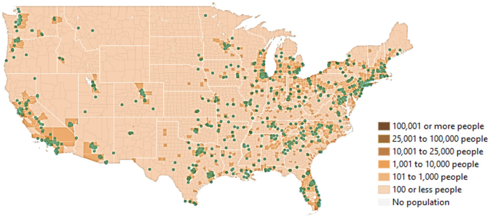
Respondents’ location on the map of U.S. population density ( 10 ).

Out of 1000 respondents who participated in our survey, 676 were eligible, and their corresponding data were used for analysis in this study. Among the 676 eligible respondents, 47% were identified as female, and 53% as male. Our sample represents more men than the U.S. population (51% females, 49% males) ( 12 ). The sample’s household income distribution is shown in Figure 2. Both mean and median income fell into the US$40,000–59,999 category, which is close to the median household income for the U.S.A. in 2018, US$61,937 ( 13 ). Figure 3 shows the sampled individuals’ educational attainment, which is skewed toward higher education than the U.S. population ( 14 ). Figure 4 illustrates the age distribution of our sample. The mean and median ages were 35 and 33 years old, respectively. The median age of U.S. individuals who are 18 years old or older is in the 45–49 years old range ( 15 ). Our sample is biased toward younger individuals compared to the national population. In the choice experiment section of the survey, respondents could have up to four trips and for each trip they could choose a mode from seven different modes available to them: regular car, self-driving car, ride-hailing, driverless ride-hailing, transit, bike, and walking. For each mode, respondents could see the travel time and applicable costs (monthly payment and parking fee for privately own vehicles, fare for ride-hailing, driverless ride-hailing, and transit). More information on experimental design can be found in Jabbari et al. ( 9 ). Before showing the scenarios, we presented respondents with a service description for the less common modes, such as ride-hailing, self- driving car, and driverless ride-hailing. Here are the descriptions with the same order and wording as presented in the survey.

Self-driving car is a car that can drive itself or be driven by a human.

Driverless car is a self-driving car with no human backup driver.

Ride-hailing services are services such as Uber and Lyft that connect passengers to local drivers to give them a ride.

Driverless ride-hailing services are services that connect passengers to driverless vehicles to give them a ride. It cannot be driven by the passenger.

Figure 2.

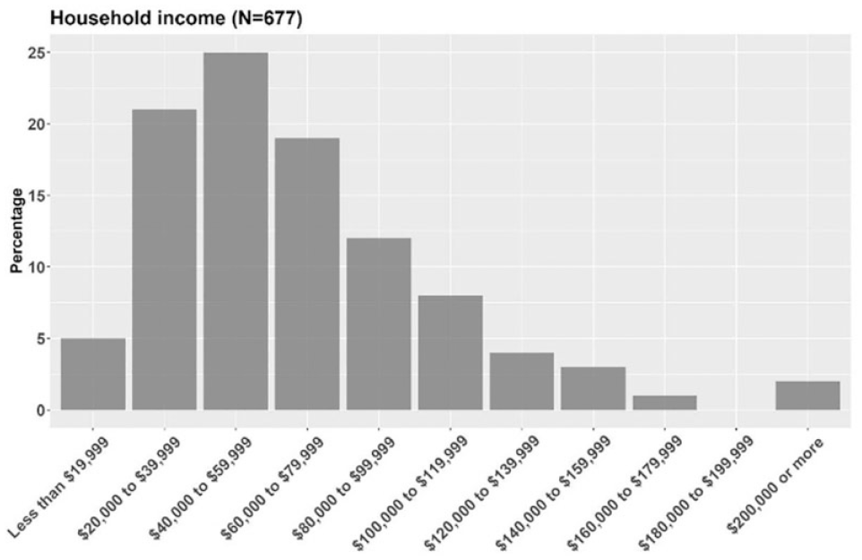
Sample’s household income.

Figure 3.

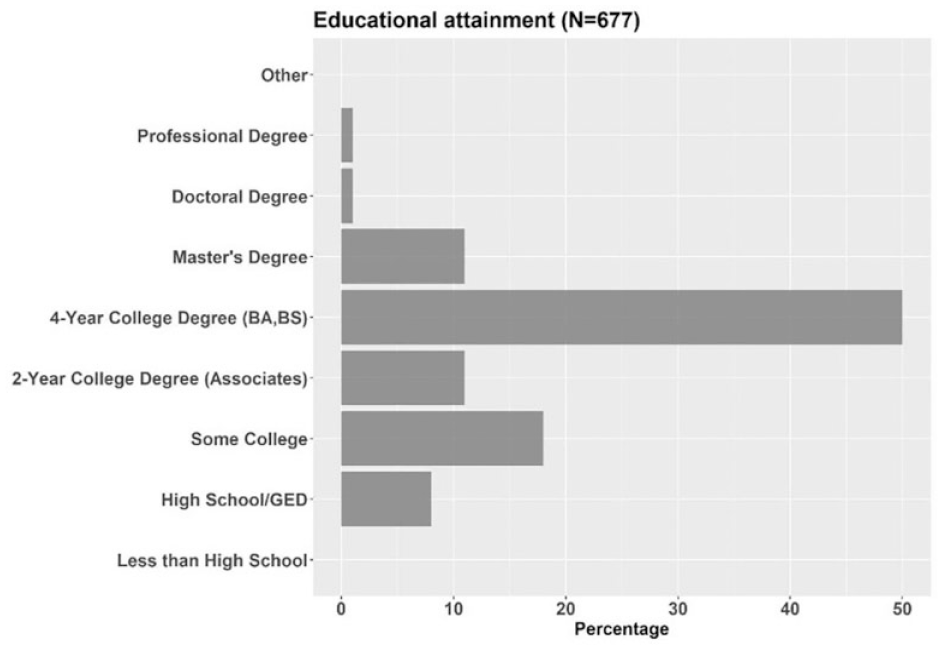
Sample’s educational attainment.

Figure 4.

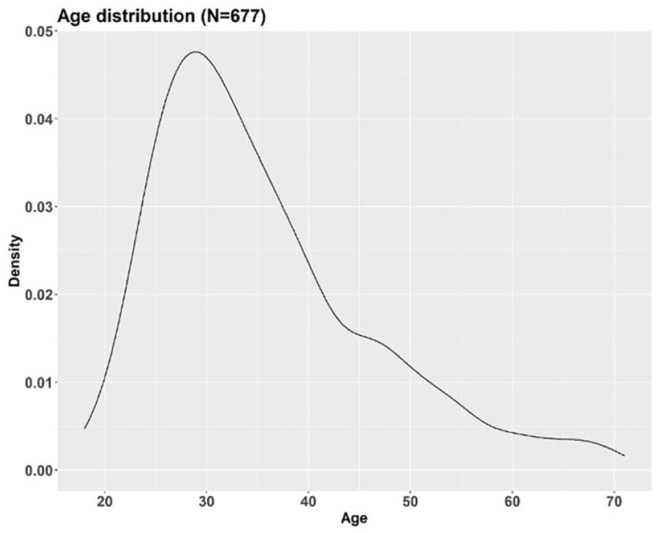
Sample’s age distribution.

Methods

We created choice experiments based on respondents’ typical workdays. Depending on their self-reported trip diary, we generated choice experiments that could include up to four trips per tour. Then we asked them to choose a mode for each trip within the tour, thus helping them to imagine their day-to-day life with the new modes, that is, self-driving car and driverless ride-hailing. Figure 5 illustrates the combinations of modes respondents chose in the choice experiment. From left to right, each column of blue bars represents trips from trip 1 to trip 4, with the height of the blue bars representing the number of people choosing each mode for that trip. The width of the grey links that connect two modes represents the number of observations with that sequence of modes. The majority of our sample reported two trips on their travel day and most of the tours are unimodal.

Figure 5.

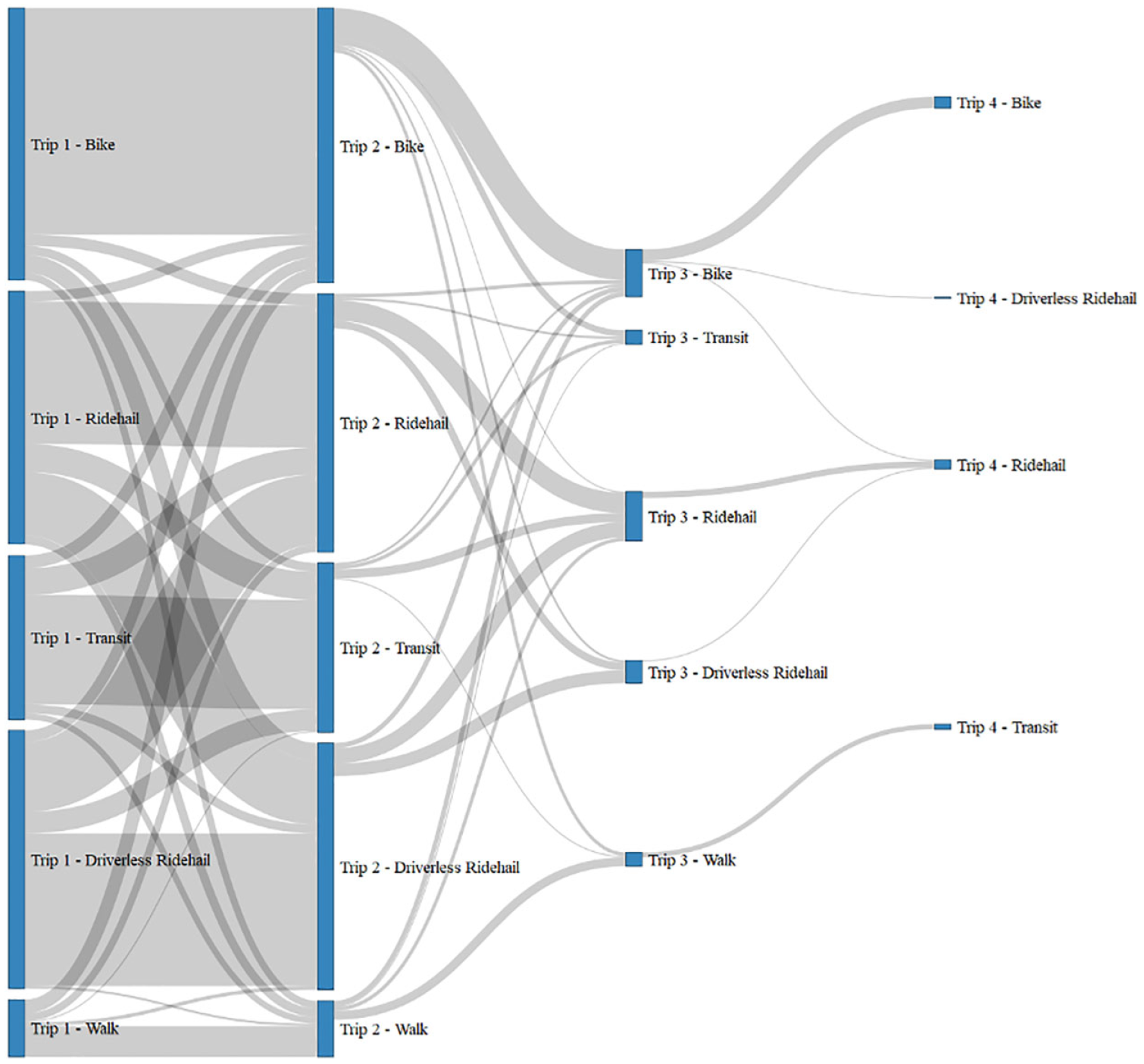
Mode choices for multimodal tours (private cars and autonomous vehicles are excluded from the diagram; color online only).

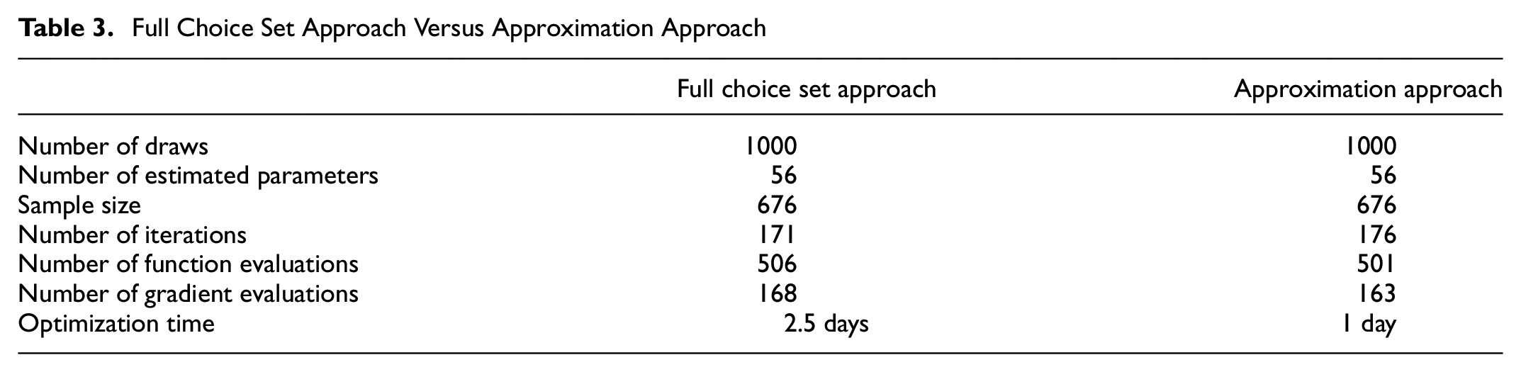
In this study, we assumed that respondents maximize their utility over the entire tour, and the total utility of the tour equals the sum of each trip’s utility ( 4 ). We used two approaches to calculate the tour utility functions. For the full choice set approach, we built a choice set of all the possible combinations of modes for tours and added the utilities of each trip in a tour to calculate the mode choice utility for that tour. If a respondent’s tour consisted of two trips, their choice set would include up to 27 options (ride-hailing, driverless ride-hailing, transit, bike, and walk for each of the two trips, plus car or self-driving car for the whole tour: 5² + 2 = 27). If their tour has four trips, their choice set could include up to 627 alternatives (5⁴ + 2 = 627). In the approximation approach, we used the expected utility of modes other than privately owned vehicles (since if respondents chose car for the first trip, they had to stick with the car for the rest of the tour) and then used the sum of the expected utilities to calculate utility for the whole tour. The approximation approach was considerably faster and computationally less intensive than the first one (more details provided in Table 3). Using the approximation approach, we built two additional models to capture interdependencies between the trips by including the prior chosen mode as a predictive variable in the utility function of the current trip, similar to autoregressive models ( 16 ). Below, we describe these models in more detail. The general utility function formula is described below:

U_{i j t} = V_{i j t} + ε'_{i j t}

(1)

V_{ijt} = β_{ij} x_{ijt} + β'_{j} x'_{ijt} + Γ_{j} x_{i}^{*} + AS C_{j}

(2)

ε'_{ijt} = φ_{ij} + ε_{ijt}

(3)

where $U_{ijt}$ is utility of mode j for individual i on trip t, $V_{ijt}$ is the deterministic part of the utility, $x_{ijt}$ indicates predictors such as travel time for which we defined alternative-specific random coefficients, $β_{ij}$ , to capture variation in taste or tolerance of the decision-maker, $x'_{ijt}$ indicates predictors such as travel cost, monthly payment for privately owned cars, parking fee, and wait time that may have alternative-specific or generic coefficients, $β'_{j}$ , $x_{i}^{*}$ is the vector of latent variables and Γ corresponds to unknown model parameters for latent variables, and $φ_{ij}$ is the mode-specific error component that captures individual i’s idiosyncratic taste variation for mode j and allows the variance of unobserved factors to vary over alternatives ( 17 ), with the exception of driverless ride-hailing. We assumed that driverless ride-hailing is correlated both with regular ride-hailing and self-driving car; therefore, instead of using an alternative-specific error component in the utility function, we used the sum of the error components for ride-hailing and for self-driving car. In addition, alternative-specific error components allow us to capture correlations between trips that have the same mode within the tour and individuals’ preferences for mode j.

Full Choice Set Approach

For this approach, we assumed respondents choose the sequence of modes that maximizes their utility over all trips in their tour. We assume that they consider each possible combination of modes (e.g., transit–transit–transit, transit–transit–ride-hailing, etc.) and that the total utility for their tour ( $U_{ir})$ is equal to sum of the utilities of the trips ( $U_{it})$ within that tour. This approach is similar to the model structure introduced by Miller et al. ( 4 ). Equation 4 shows this relationship:

U_{ir} = \sum_{t}^{T_{r}} U_{it}

(4)

The utility of tour r for person i, $U_{ir}$ , is sum of the trips’ utilities, $U_{it}$ , within the tour. The utility of each trip depends on the mode chosen, as shown in Equations 1–3. Each person has T_r trips within the tour and T_r can range between two and four trips. Therefore, the number of alternatives in the choice set for each person depends on the number of trips they had in their tour and the availability of the modes for each trip.

Tours start from home and there were seven modes in the choice set for each trip: car, self-driving car, walking, biking, transit, ride-hailing, and driverless ride-hailing. If respondents chose any of the other non-car modes for the first trip, they could not choose the car or self-driving car option for the remaining trips.

Approximation Approach

As the number of trips within the tour increases, it is more burdensome to generate all the possible mode combinations and estimating the model becomes computationally more intensive. To alleviate the model estimation complexity, we used the approximation approach where expected utilities for modes other than privately owned options (car and self-driving car) were computed. In this approach, we calculated the final probabilities in two steps. Except for privately owned vehicles, the other five modes were allowed to be chosen in any trip, conditional on the first trip’s mode being anything other than a regular or self-driving private car. “Other” modes include biking, walking, ride-hailing, driverless ride-hailing, and transit. In the first step, we calculated the expected utility of choosing “other” modes for each trip, as shown in the following equation:

\begin{matrix} V_{it, other} = \log \sum_{j}^{J} e^{V_{ijt}}; j \in J = {biking, walking, ride \\ - hailing, driverless ridehailing, transit} \end{matrix}

(5)

After that, we added the expected utilities as the total utility of choosing “other” modes for the tour. Below, we formulated this approach. Utility functions for choosing a regular car, a self-driving car, and other modes for tour r and person i are as below:

V_{ir, car} = \sum_{t}^{T_{r}} V_{it, car}

(6)

V_{ir, self - driving car} = \sum_{t}^{T_{r}} V_{it, self - driving car}

(7)

V_{ir, other} = \sum_{t = 1}^{T_{r}} V_{it, other}

(8)

Intuitively, the approximation approach can be understood as separating each tour into a series of (conditionally) independent trips. The expected utility of each trip is calculated based on the attributes of modes available for that trip, and the total utility for the tour is the sum of these expectations.

Autoregressive Models

In the choice experiment, participants could see the whole tour and mode options and their attributes all at once. There was no uncertainty about future modes and their attributes. As discussed earlier, one possible thought process of the respondents could be maximizing the utility of each trip (which was captured through the previous two models) by making a decision solely based on the available options for each given trip. Another thought process could be considering their mode choices of previous trips when choosing a mode for the current trip. In other words, they may demonstrate forward-looking behavior in the experimental setting. To capture such behavior, we added an autoregressive variable to the utility function of the modes that are not privately owned vehicles. Equations 9 and 10 show the utility function formula for two different model specifications with autoregressive variables:

U_{ijt} = V_{ijt} + ρ y_{it - 1} + ε'_{ijt}

(9)

U_{ijt} = V_{ijt} + ρ_{j} y_{it - 1} + ε'_{ijt}

(10)

where

ε'_{ijt} = φ_{ij} + ε_{ijt}

(11)

where $U_{ijt}$ is the utility of mode j for individual i on trip t and $V_{ijt}$ is the deterministic part of the utility. We assumed that the current level of utility of mode j is partly dependent on the previously chosen mode. Here, $ρ and ρ_{j}$ are weights that measure the effect of choosing mode j for trip t–1 on choosing mode j for trip t and it is the same for each individual, $ρ$ is a generic variable (one variable is estimated for all the modes) and $ρ_{j}$ is an alternative-specific variable (different variables are estimated for different modes), and $y_{it - 1}$ is a dummy variable with value 1 if mode j is chosen on trip t–1 and 0 otherwise. The error term $ε'_{ijt}$ captures unobserved factors. The assumption of independence of the error terms $ε'_{ij (t - 1)}$ and $ε'_{ijt}$ is relaxed since we replace the error term $ε'_{ijt}$ with the sum of two error terms as described previously. Further, $φ_{ij}$ captures the preferences of individual i for mode j.

ICLV Framework

An ICLV model allows latent (not directly observable) psychometric constructs to be used alongside observable attributes of alternatives to predict choice behavior. In a prior study, Jabbari et al. ( 10 ), we identified two latent variables—the perception of safety of AVs and the importance of car ownership—that significantly affected mode choices. Therefore, we included these two latent variables in the tour-based mode choice models as well. (This is not to imply that these are the only two latent constructs affecting mode choice in general, but they are the two found to be significant predictors of mode choice in prior work using a subset of the present data.) We used an ICLV framework similar to that reported by Jabbari et al. ( 10 ), which was adapted from Vij and Walker ( 18 ).

The ICLV framework consisted of two main components: (1) a discrete choice sub-model and (2) a latent variable sub-model. Each of the sub-models includes a structural and a measurement component ( 18 ). Under the random utility maximization (RUM) framework, the standard choice model is a latent variable model itself. Utility is a latent construct that measures an individual’s satisfaction conditional on the attributes of each alternative. Structural equations describe the latent variables with respect to observable exogenous variables, and measurement equations link latent variables to observable indicators. For the latent variable sub-model, indicators can be responses to psychometric questions. For the choice model, the indicator is the decision-maker’s choice (whether revealed or stated) ( 18 , 19 ).

Structural Equations

The structural equations are as follows:

V_{ijt} = β x'_{ijt} + Γ x_{i}^{*}

(12)

x_{i}^{*} = A x_{i} + υ_{i}

(13)

Measurement Equations

The measurement equations are as follows:

\begin{matrix} I_{i} = {Dx}_{i}^{*} + ζ_{i} \\ y_{ijt} = {\begin{matrix} 1 if U_{ijt} \geq U_{i j^{″} t} \\ 0 otherwise \end{matrix} for j^{″} \neq j \end{matrix}

(14)

\begin{matrix} j, j ″ \in {biking, walking, ride - hailing, driverless ride \\ - hailing, transit, car, self - driving car} \end{matrix}

(15)

where $V_{ijt}$ is the deterministic part of the utility for mode j for individual i on trip t, $x_{i}$ and $x'_{ijt}$ are observable explanatory variables and $x_{i}^{*}$ is a latent variable, $β$ and $Γ$ are unknown model parameters corresponding to observable and latent variables, respectively, A is the parameter that indicates the structural relationship between the latent and observable variables, and $υ_{i}$ is the stochastic component of that relationship from a normal distribution.

The measurement model links the latent variables to indicators, where $I_{i}$ corresponds to the indicators used to measure the latent variables for the decision-maker i. Table 1 shows the psychometric questions that were used as latent variable indicators. For more information on how these questions were selected, please refer to Ge et al. ( 11 ) and Jabbari et al. ( 10 ). Here, D is the unknown parameter that indicates the relationship between indicators and latent variables, and $ζ_{i}$ is a vector of measurement equation error terms that are normally distributed; Equation 15 connects utility to the choice indicator, $y_{ijt}$ ( 18 ).

Table 1.

Psychometric Questions Used as Latent Variable Indicators

Indicators
Safety perception of AVs
I am ______ self-driving vehicles can drive as well as human drivers in general. (1- Extremely doubtful, 2- Doubtful, 3- A little doubtful, 4- Sort of confident, 5- Confident, 6- Extremely confident)
Driverless cars generally will be ______compared with most drivers on the road. (1- Much more dangerous, 2- More dangerous, 3- Somewhat more dangerous, 4- A little safer, 5- Safer, 6- Much safer)
Widespread use of self-driving vehicles would result in ______crashes. (1- A lot more, 2- More, 3- Slightly more, 4- Slightly fewer, 5- Fewer, 6- A lot fewer)
Driverless cars generally will be ______than I am as a driver. (1- Much more dangerous, 2- More dangerous, 3- Somewhat more dangerous, 4- A little safer, 5- Safer, 6- Much safer)
I ______trust self-driving car technology to keep me safe when I am riding in one. (1- Definitely would not, 2- Probably would not, 3- Maybe would not, 4- Maybe would, 5- Probably would, 6- Definitely would)
Car ownership importance
Owning a car is a(n) ______part of being an adult. (1- Not important at all, 2- Not important, 3- Not so important, 4- Somewhat important, 5- Very important, 6- Extremely important)
Owning a car I can use anytime is ______. (1- Not at all important, 2- Not important, 3- Not so important, 4- Somewhat important, 5- Very important, 6- Extremely important)
Driving my own car is ______ . (1- Not empowering at all, 2- Not empowering, 3- Not so empowering, 4- Somewhat empowering, 5- Very empowering, 6-Extremely empowering)
The flexibility of driving by myself is ______. (1- Not at all important, 2- Not important, 3- Not so important, 4- Somewhat important, 5- Very important, 6- Extremely important)
The ability to make spontaneous stops when I drive my own car is ______ to me. (1- Not at all important, 2- Not important, 3- Not so important, 4- Somewhat important, 5- Very important, 6- Extremely important)

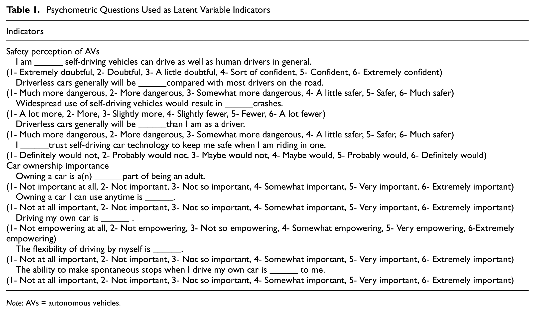
Note: AVs = autonomous vehicles.

The model system was estimated using simultaneous estimation in PandasBiogeme ( 20 ). Simultaneous estimation is preferred when feasible for its greater flexibility and efficiency compared with sequential estimation ( 21 ). Some 1000 Halton draws were used for calculating the maximum simulated likelihood.

Results/Discussion

Table 2 shows the results of the three models and also the model from our previous paper, Jabbari et al. ( 10 ), for the purpose of comparison. We cannot directly compare the model from Jabbari et al. ( 10 ) with the models in this paper since the sample size is quite different. The reason for this difference in sample sizes is that in the present work we had to remove some of the observations that had issues in the second to fourth trips of their tour. For a discussion of latent variables please refer to Jabbari et al. ( 10 ).

Table 2.

Tour-Based Models Result (Numbers in Parenthesis are the Standard Error of Estimations)

		Jabbari et al. ( 10 )	This work
		First trip only	Full tour
			Full choice set approach	Approximation approach
			Without autoregressive variables (model 1)	Without autoregressive variables (model 2)		One autoregressive variable (model 3)		Alternative-specific autoregressive variables (model 4)
Variable		Estimate	Estimate	Estimate		Estimate		Estimate
Car
Monthly payment/monthly income		−3.08*** (0.41)	−3.06*** (0.41)	−3.07*** (0.41)		−3.60*** (0.44)		−3.63*** (0.44)
Parking fee/daily income		−6.60* (2.84)	−2.47 (2.51)	−2.94 (2.53)		−2.00 (2.71)		−2.24 (2.71)
Travel time (h)	MeanSD	−2.00*** (0.32)	−1.07*** (0.16)	−1.07*** (0.17)		−1.29*** (0.18)		−1.28*** (0.18)
Travel time (h)		2.27***(0.42)	0.09(0.20)	0.21(0.19)		0.47*(0.20)		0.47*(0.20)
Alternative-specific constant		0.98***(0.27)	0.56*(0.23)	0.56*(0.24)		0.15(−0.35)		0.26(0.35)
Error component		na	0.20(0.18)	0.17(0.17)		0.18(0.21)		0.16(0.21)
Car ownership importance		1.22***(0.14)	2.11***(0.31)	2.07***(0.30)		3.09***(0.41)		3.09***(0.41)
Self-driving car
Monthly payment/monthly income		−3.08***(0.41)	−3.06***(0.41)	−3.07***(0.41)		−3.60***(0.44)		−3.63***(0.44)
Parking fee/daily income		−6.60*(2.84)	−2.47(2.51)	−2.94(2.53)		−2.00(2.71)		−2.24(2.71)
Travel time (h)	MeanSD	−2.35***(0.43)	−1.18***(0.18)	−1.19***(0.18)		−1.46***(0.20)		−1.45***(0.20)
Travel time (h)		3.21***(0.52)	0.01(0.22)	0.30(0.20)		0.57*(0.22)		0.56*(0.22)
Alternative-specific constant		0.16(0.28)	−0.19(0.24)	−0.23(0.25)		−0.58(0.36)		−0.48(0.35)
Error component		na	0.22(0.17)	0.13(0.15)		0.41(0.21)		0.40(0.21)
Safety of AVs		0.46***(0.04)	0.16***(0.04)	0.20***(0.04)		0.18***(0.05)		0.20***(0.04)
Car ownership importance		1.22***(0.14)	2.11***(0.31)	2.07***(0.30)		3.09***(0.41)		3.09***(0.41)
Driverless ride-hailing
Cost/daily income		−5.21***(0.69)	−0.69***(0.19)	−0.73***(0.19)		−0.73***(0.18)		−0.73***(0.18)
Wait Time (h)		0.01(0.02)	−0.31(0.48)	−0.32(0.47)		−0.24(0.55)		−0.31(0.54)
Travel time (h)	MeanSD	−1.55***(0.53)	−0.49*(0.24)	−0.48*(0.23)		−0.60*(28)		−0.59*(0.27)
Travel time (h)		0.17(0.53)	0.25(0.29)	0.48(0.27)		−0.19(0.32)		0.19(0.32)
Alternative-specific constant		−0.83***(0.30)	−1.87***(0.39)	−1.94***(0.37)		−3.47***(0.59)		−3.36***(0.58)
Safety of AVs		0.46***(0.04)	0.16***(0.04)	0.20***(0.04)		0.18***(0.05)		0.18***(0.05)
Car ownership importance		0.81***(0.17)	2.53***(0.66)	2.58***(0.648)		4.84***(1.00)		4.83***(0.99)
Previous mode: driverless ride-hailing		na	na	na		3.50***(0.09)		3.18***(0.15)
Ride-hailing
Cost/daily income		−5.21***(0.69)	−0.69***(0.19)	−0.73***(0.19)		−0.73***(0.18)		−0.73***(0.18)
Wait time (h)		0.01(0.02)	−0.31(0.48)	−0.32(0.47)		−0.24(0.55)		−0.31(0.54)
Travel time (h)	MeanSD	−4.42***(0.89)	−0.79**(0.25)	−0.78***(0.25)		−0.83**(0.26)		−0.81**(0.25)
Travel time (h)		2.44***(0.68)	0.33(0.24)	0.50(0.23)		0.63*(0.29)		0.61*(0.29)
Alternative-specific constant		0.16(0.28)	−1.1**(0.37)	−1.21***(0.34)		−2.08***(0.50)		−1.98***(0.49)
Error component		na	0.01(011)	0.04(0.10)		−0.13(0.14)		0.13(0.14)
Car ownership importance		0.57***(0.17)	1.79**(0.58)	1.92***(0.54)		3.20***(0.78)		3.18***(0.77)
Previous mode: ride-hailing		na	na	na		3.50***(0.09)		3.19***(0.16)
Transit
Cost/daily income		−5.21***(0.69)	−0.69***(0.19)	−0.73***(0.19)			−0.73***(0.18)	−0.73***(0.18)
Wait time (h)		0.03(0.02)	−0.90(1.01)	−1.20(1.00)			−0.62(1.19)	−0.57(1.2)
Travel time (h)	MeanSD	−2.97***(0.55)	−0.27***(0.07)	−0.28***(0.07)			−0.34***(0.07)	−0.34***(0.07)
Travel time (h)		1.92***(0.35)	0.19**(0.06)	0.20***(0.06)			0.20***(0.08)	0.20***(0.06)
Previous mode: transit		na	na	na			3.50***(0.09)	3.75***(0.21)
Bike
Travel time (h)	MeanSD	−10.80***(1.28)	−1.55***(0.15)	−1.74***(0.16)		−2.04***(0.21)		−2.04***(0.22)
Travel time (h)		6.50***(0.74)	0.42(0.26)	0.69***(0.10)		1.12***(0.13)		1.12***(0.13)
Alternative-specific constant		2.63***(0.29)	0.78***(0.19)	0.82***(0.19)		0.83***(0.23)		0.77**(0.24)
Error component		na	0.53**(0.16)	0.05***(0.10)		0.63***(0.11)		0.63***(0.12)
Previous mode: bike		na	na	na		3.50***(0.09)		4.25***(0.20)
Walk
Travel time (h)	MeanSD	−55.80***(13.10)	−2.06*(0.42)	−2.63***(0.34)	−3.53***(0.55)			−3.54***(0.55)
Travel time (h)		30.90***(7.18)	0.96*(0.18)	1.14***(0.14)	1.89***(0.29)			1.91***(0.29)
Alternative-specific constant		5.08***(0.59)	0.17(0.30)	0.47(0.25)	0.87**(0.33)			0.95**(0.34)
Error component		na	0.52**(0.17)	0.48***(0.15)	1.34***(0.18)			1.35***(0.18)
Previous mode: walk		na	na	na	3.50***(0.09)			3.17***(0.35)
Null log-likelihood		−18,684.46	−22,014.13	−22,014.16	−22,014.16			−22,014.16
Final log-likelihood		−13,303.33	−13,763.41	−13,754.47	−12,746.61			−12,732.87
Adjusted rho-square		0.285	0.372	0.373	0.418			0.419
Akaike information criterion		26,708.66	27,638.81	27,620.95	25,607.23			25,587.73
Bayesian information criterion		26,944.49	27,891.72	27,873.85	25,864.65			25,863.22
Number of draws		2000	1000	1000	10000			1000
Number of estimated parameters		51	56	56	57			61
Sample size		753	676	676	676			676

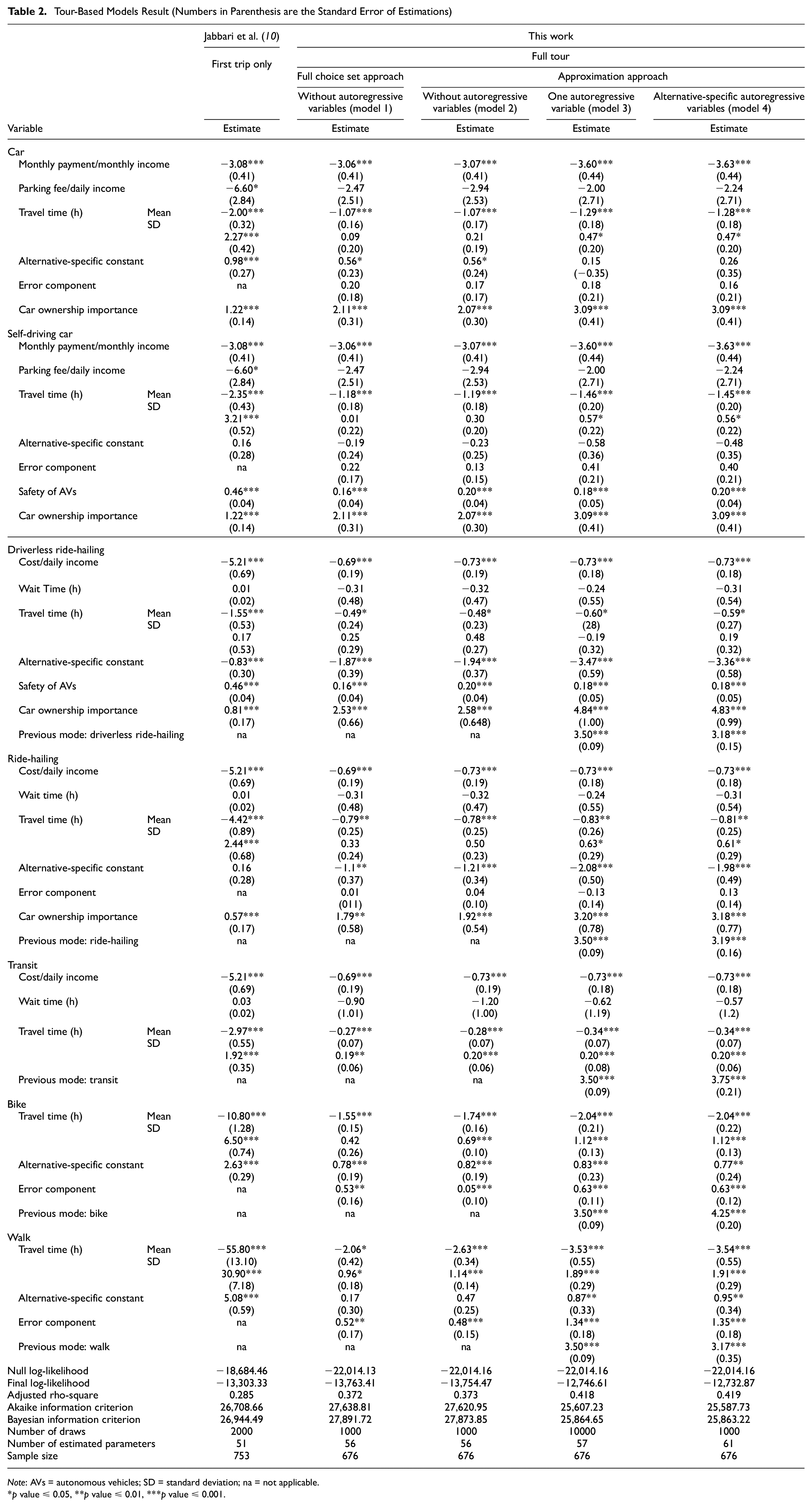
Note: AVs = autonomous vehicles; SD = standard deviation; na = not applicable.

p value ≤ 0.05, **p value ≤ 0.01, ***p value ≤ 0.001.

The full choice set approach and the approximation approach are different in their probability calculations. In the former, individuals could have up to 627 alternatives in each choice situation if they had four trips in their travel day. However, in the latter, instead of using one choice consisting of all the possible mode combinations, we summed the expected utility of trips to find the probability of each tour. The final log-likelihoods for models without autoregressive variables using these two approaches are somewhat close, but the approximation approach has a slightly higher log-likelihood. Estimated coefficients are also close in their magnitude when comparing these two approaches. Table 3 shows the optimization time and other statistics for the two approaches. The approximation approach is considerably faster than the full choice set approach. This suggests that the approximation approach provides similar results to the full choice set approach, but is more efficient and scalable. The number of choice options for the full choice set approach is kⁿ (n: number of trips and k: number of modes available). Adding one more trip to the tour or one more mode to the mode set would drastically change the number of utility functions that need to be calculated for the full choice set approach, likely rendering it impractical for anything larger than the numbers of trips and modes investigated here. We conclude that the approximation approach is a reasonable substitute for the full choice set approach.

Table 3.

Full Choice Set Approach Versus Approximation Approach

	Full choice set approach	Approximation approach
Number of draws	1000	1000
Number of estimated parameters	56	56
Sample size	676	676
Number of iterations	171	176
Number of function evaluations	506	501
Number of gradient evaluations	168	163
Optimization time	2.5 days	1 day

We conducted a likelihood ratio test to compare models without autoregressive variables and models with autoregressive variables. The model without autoregressive variables is rejected when compared to the model with one autoregressive variable ( $χ^{2} = 2016 > 3.84$ ), and the model with one autoregressive variable is rejected compared to the model with alternative-specific autoregressive variables ( $χ^{2} = 28 > 9.48$ ). This indicates that the model with alternative-specific autoregressive variables describes the data better than the model with one autoregressive variable, which itself describes the data better than the model with no autoregressive variables.

The estimated parameters for regular car and self-driving car are similar in all five models. One main difference is that the parking fee is not a statistically significant variable in the tour-based models. This may be because the parking fee is influential for a single trip, but it does not affect individuals’ decision to take a personal car for a whole tour. On the other hand, car ownership importance is highly significant in all models. However, its effect has grown relative to the monthly payment in the tour-based models. This highlights the critical role cars play when individuals plan for more than one trip.

Comparing the magnitude of coefficients for parameters of the other modes is rather difficult because not only has the model specification been modified in the tour-based models compared to the trip-based model, but also the number of observations for the models was different. In the trip-based model, we focused on the tour’s first trip. Respondents may have chosen a mode for the first trip because they optimized some of the tour-level variables. For example, they may aim not to exceed more than a certain number of minutes in time or dollars in cost for the whole tour. Therefore, respondents may consider those thresholds when making decisions for trips. In the trip-based model, we could not capture these interdependencies, which may be reflected in the estimated coefficients.

One point to highlight here is that unlike the model from our previous work ( 10 ), car ownership importance for different modes from the tour-based model cannot be compared since they are estimated differently. For example, in a tour with four trips, the tour utility functions for privately owned cars are equal to the sum of each mode’s utilities (in all models), meaning that the car ownership importance variable is included in the tour utility four times. However, for the case of ride-hailing modes, depending on how many times ride-hailing modes are included in the mode combination, car ownership importance could be included once or up to four times. Therefore, the car ownership importance representation is not balanced between privately owned vehicles and ride-hailing services and should not be compared.

The significance of the autoregressive variables indicates a “mode inertia” among our respondents. Results suggest that individuals are inclined to use the same mode for consecutive trips in a travel day, and they gain higher utility from this repetition than from using a new mode. The magnitudes of these autoregressive effects are weakest for walking, ride-hailing, and driverless ride-hailing (3.17–3.19) and strongest for cycling (4.25).

To better understand and validate the mode inertia identified in our model, we compared our survey with revealed preference data from the National Household Travel Survey (NHTS). Our goal was to understand whether the tendency to choose repeated modes within tours was specific to our sample or also exists in the NHTS. To achieve this, we first identified tours within the NHTS data. We assumed that a tour includes at least two trips. When there were sequential trips that started and ended at home, we assumed those trips, and all the trips in between, were all within one tour. If the last trip of the day did not end at home, we assumed that the tour ended with the last trip. Then, we looked at tours and the combinations of modes used for them. We only considered tours that included at least one trip with a mode other than a car (since in this work we used autoregressive variables only for non-car modes). We also removed tours that included one or more trips by airplane, as their nature is quite different from what we are interested in here. We identified 41,614 tours in the 2017 NHTS. Of these, 58% of the tours were unimodal, using walk, bike, public transportation, or taxi/ride-hailing modes. In our choice experiment, a similar fraction of non-private-auto tours—63%—were unimodal.

Conclusions

In this paper, we developed four tour-based models using two approaches to formulate probability and two model specifications. The purpose of undertaking two different approaches for formulating probability was to determine whether there is a less computationally intense approach to estimate tour-based models with a higher number of trips within the tour. The purpose of using two model specifications was to explore whether the previous trip’s mode choice affects the choice of mode for the current trip.

We found that using the approximation approach and expected utilities for “other” modes (e.g., walk, bike, transit, ride-hailing, driverless ride-hailing) and calculating utilities in two steps (model 2) performed better than the model in which we enumerated all possible combinations of available modes as the choice set and summed the utility of trips within the tour to calculate the utility of the tour (model 1). When we added autoregressive variables to capture the effect of choosing the same mode as the prior trip, we found that the model improved in performance. Also, the likelihood ratio test rejects the null hypothesis that coefficients for autoregressive variables are zero. We discovered a considerably high “mode inertia” among our sample, meaning that when choosing the same mode as the previous trip for the next trip, the utility of that mode goes up considerably, and this finding is consistent for all the modes (excluding personal vehicle options, for which it was assumed that the vehicle must be used for all trips in the tour). This finding indicates that respondents in our sample were more likely to stick with unimodal tours than multimodal ones.

To understand whether this finding is unique to our sample of individuals or is consistent with other datasets, we looked at the 2017 NHTS. After processing the trips and identifying tours, we found a similar pattern in the NHTS data—most tours were unimodal. This is an important finding since decision-makers and experts have made tremendous efforts to promote multimodal travel as a vital component of sustainable urban mobility in the future ( 22 ). However, our findings show that despite providing a wide variety of modal alternatives (including driverless ride-hailing) and presenting full information about the available modes’ attributes, there was a strong inclination toward unimodal travel behavior. It may be necessary to temper expectations about the prospects of multimodal travel even in a future where mode options can be readily displayed and compared side by side. Kent ( 22 ) found that time competitiveness is not enough motivation for travelers to switch from personal vehicles to alternative modes. “Flexibility, freedom, and reliability, as well as the interminable pull of the sensory experience provided by the cocoon of the car,” are the main barriers for the widespread use of alternate modes. Another study highlighted that old age, employment, more children, higher income, and higher car availability resulted in a lower probability of adopting multimodality, while higher availability of biking and transit infrastructure increased the probability of multimodal travel ( 23 ). Intuitively, the factors identified by Klinger ( 23 ) are predictors of how individuals prioritize between flexibility and freedom and mode attributes such as travel time and cost. For future research, it might be useful to explore how people with different sociodemographics perceive modes other than a personal vehicle with respect to reliability and flexibility. In addition, the data used in this study are based on individuals’ typical workdays. However, evidence shows that alternative modes are primarily used for specific purposes, whereas personal vehicles are used for all types of purposes ( 24 ).

Footnotes

Author Contributions

The authors confirm contribution to the paper as follows: study conception and design: P. Jabbari, D. MacKenzie; data collection: P. Jabbari; analysis and interpretation of results: P. Jabbari, D. MacKenzie; draft manuscript preparation: P. Jabbari, D. MacKenzie, N. Khan. All authors reviewed the results and approved the final version of the manuscript.

Declaration of Conflicting Interests

The author(s) declared no potential conflicts of interest with respect to the research, authorship, and/or publication of this article.

Funding

The author(s) disclosed receipt of the following financial support for the research, authorship, and/or publication of this article: The work described here was sponsored by the U.S. Department of Energy (DOE) Vehicle Technologies Office (VTO) under the Systems and Modeling for Accelerated Research in Transportation (SMART) Mobility Laboratory Consortium, an initiative of the Energy Efficient Mobility Systems (EEMS) Program.

ORCID iDs

Parastoo Jabbari

Nazmul Arefin Khan

Don MacKenzie

The submitted manuscript has been created by University of Washington and the UChicago Argonne, LLC, Operator of Argonne National Laboratory (Argonne). Argonne, a U.S. Department of Energy Office of Science laboratory, is operated under Contract No. DE-AC02-06CH11357. The U.S. Government retains for itself, and others acting on its behalf, a paid-up nonexclusive, irrevocable worldwide license in said article to reproduce, prepare derivative works, distribute copies to the public, and perform publicly and display publicly, by or on behalf of the Government.

References

Ben-Akiva

Bowman

Ramming

Walker

Behavioral Realism in Urban Transportation Planning Models. Proc., Transportation Models in the Policy-Making Process: A Symposium in Memory of Greig Havey, Asilomar Conference Center, California, 1998.

Kagerbauer

Hilgert

Schroeder

Vortisch

Household Travel Survey of Intermodal Trips – Approach, Challenges and Comparison. Transportation Research Procedia, Vol. 11, 2015, pp. 330–339. https://doi.org/10.1016/j.trpro.2015.12.028.

Clifton

Muhs

Capturing and Representing Multimodal Trips in Travel Surveys: Review of the Practice. Transportation Research Record: Journal of the Transportation Research Board, 2012. 2285: 74–83.

Miller

E. J.

Roorda

M. J.

Carrasco

J. A.

A Tour-Based Model of Travel Mode Choice. Transportation, Vol. 32, No. 4, 2005, pp. 399–422. https://doi.org/10.1007/s11116-004-7962-3.

Frank

Bradley

Kavage

Chapman

Lawton

T. K.

Urban form, Travel Time, and Cost Relationships with Tour Complexity and Mode Choice. Transportation, Vol. 35, No. 1, 2008, pp. 37–54. https://doi.org/10.1007/s11116-007-9136-6.

Roorda

M. J.

Passmore

Miller

E. J.

Including Minor Modes of Transport in a Tour-Based Mode Choice Model with Household Interactions. Journal of Transportation Engineering, Vol. 135, No. 12, 2009, pp. 935–945. https://doi.org/10.1061/(ASCE)TE.1943-5436.0000072.

Bastarianto

F. F.

Irawan

M. Z.

Choudhury

Palma

Muthohar

A Tour-Based Mode Choice Model for Commuters in Indonesia. Sustainability, Vol. 11, No. 3, 2019, p. 788. https://doi.org/10.3390/su11030788.

Mulley

Tour-Based Mode Choice of Joint Household Travel Patterns on Weekend and Weekday. Transportation, Vol. 40, No. 4, 2013, pp. 789–811.

Jabbari

Ranjbari

MacKenzie

Using a Tour-based Model to Understand Mode Choice Effects of Vehicle Automation. Presented at 99th Annual Meeting of the Transportation Research Board, Washington, D.C., 2020.

10.

Jabbari

Auld

MacKenzie

How Do Safety Perceptions of safety and Car Ownership Importance Affect Autonomous Vehicle Adoption?

Travel Behaviour and Society, Vol. 28, 2022, pp. 128–140. https://doi.org/10.1016/j.tbs.2022.02.002.

11.

Ranjbari

Lewis

E. O.

Barber

MacKenzie

Defining Psychometric Variables Related to Use of Autonomous Vehicles. Transportation Research Record: Journal of the Transportation Research Board, 2019. 2673: 655–669.

12.

U.S. Census Bureau. National Population by Characteristics: 2010-2019. The United States Census Bureau, 2019. https://www.census.gov/data/tables/time-series/demo/popest/2010s-national-detail.html.

13.

Haboucha

C. J.

Ishaq

Shiftan

User Preferences Regarding Autonomous Vehicles. Transportation Research Part C: Emerging Technologies, Vol. 78, 2017, pp. 37–49. https://doi.org/10.1016/j.trc.2017.01.010

14.

Lavieri

P. S.

Bhat

C. R.

Modeling Individuals' Willingness to Share Trips with Strangers in an Autonomous Vehicle Future. Transportation Research Part A: Policy and Practice, Vol. 124, 2019, pp. 242–261. https://doi.org/10.1016/j.tra.2019.03.009

15.

Wicki

Guidon

Becker

Axhausen

K. W.

Bernauer

How Technology Commitment Affects Willingness to use AVs: Results from Realistic Mode Choice Experiment for a Self-Driving Shuttle Service. Research in Transportation Business & Management, Vol. 49, 2019, p. 29.

16.

Rahimi

Azimi

Jin

Examining juman Attitudes Toward Shared Mobility Options and Autonomous Vehicles. Transportation Research Part F: Traffic Psychology and Behaviour. Vol. 72, 2020, pp. 133–54.

17.

Train

Discrete Choice Methods with Simulation. Cambridge University Press, 2002. https://eml.berkeley.edu/books/choice2.html.

18.

Vij

Walker

J. L.

Integrated Choice and Latent Variable Models: Holy Grail, or Not?

Proc., International Choice Modelling Conference, International Choice Modelling Conference, May 11, Austin, TX, 2015.

19.

Bolduc

Alvarez-Daziano

On Estimation of Hybrid Choice Models. In Choice Modelling: The State-of-the-Art and the State-of-Practice (S. Hess and A. Daly, eds.), Emerald Group Publishing Limited, Bingley, 2010, pp. 259–287. https://doi.org/10.1108/9781849507738-011.

20.

Bierlaire

A Short Introduction to PandasBiogeme. Technical Report TRANSP-OR 200605. Transport and Mobility Laboratory, ENAC, EPFL, 2020.

21.

Raveau

Álvarez-Daziano

Yáñez

M. F.

Bolduc

De Dios Ortúzar

Sequential and Simultaneous Estimation of Hybrid Discrete Choice Models: Some New Findings. Transportation Research Record: Journal of the Transportation Research Board, 2010. 2156: 131–139.

22.

Kent

J. L.

Driving to Save Time or Saving Time to Drive? The Enduring Appeal of the Private Car. Transportation Research Part A: Policy and Practice, Vol. 65, 2014, pp. 103–115. https://doi.org/10.1016/j.tra.2014.04.009.

23.

Klinger

Moving from Monomodality to Multimodality? Changes in Mode Choice of New Residents. Transportation Research Part A: Policy and Practice, Vol. 104, 2017, pp. 221–237. https://doi.org/10.1016/j.tra.2017.01.008.

24.

Kuhnimhof

Chlond

Von Der Ruhren

Users of Transport Modes and Multimodal Travel Behavior: Steps Toward Understanding Travelers’ Options and Choices. Transportation Research Record: Journal of the Transportation Research Board, 2006. 1985: 40–48.

Evidence for Modal Inertia in Multimodal Tours: An Integrated Choice and Latent Variable Modeling Approach

Abstract

Keywords

Data

Methods

Full Choice Set Approach

Approximation Approach

Autoregressive Models

ICLV Framework

Structural Equations

Measurement Equations

Results/Discussion

Conclusions

Footnotes

Author Contributions

Declaration of Conflicting Interests

Funding

ORCID iDs

References