
Abstract
Assigning inspection trains to monitor track quality is a standard procedure for maintaining railway system safety. The main challenges lie in lacking time and resources to perform the inspections because of the increasing traffic nowadays. To overcome these challenges, many consider adopting the on-board monitoring (OBM) technique for performing the inspections. This technique assigns commercial trains, instead of traditional track recording vehicles (TRVs), to monitor the track status, allowing railway operators to perform more inspections without affecting the traffic and using expensive inspection trains as well. However, compared with TRV data, the new OBM data are of lower data quality and have fewer features, although they can be recorded more frequently. Therefore, new methods should be developed for effectively applying the new data. This study develops four models, namely the linear regression model, Markov model, ordinary Kriging model, and Kalman filter model, for predicting the track status based on the OBM data. Data collected from the Switzerland railway network are used for verifying the models. Results show that the proposed models can effectively predict the degradation of the track status in different ways and, therefore, assist railway operators in scheduling maintenance tasks.
Assigning track recording vehicles (TRVs) to monitor track quality is a standard procedure for maintaining railway system safety. Railway operators usually schedule TRVs to monitor the railway network and use the recorded data for future prediction ( 1 ). However, railway operators nowadays face a lack of time and resources for performing inspections because of the increasing demand. Take Switzerland as an example: by 2040, railway passenger transport is expected to increase by 51% ( 2 ). The expectation of increasing demand triggers the need for a more efficient way of monitoring the track status.
To deal with these problems, railway operators are investing in new methods for monitoring the track status of the railway network. One possible way is to apply on-board monitoring (OBM) techniques for monitoring the track status ( 3 ). The main concept for the OBM technique is to use commercial trains, instead of TRVs, for monitoring the track status. For example, the OBM data applied in this study was collected by accelerometer sensors implemented on axles, bogies, and car bodies. The collected acceleration data can be transferred into alignment and longitudinal defects data based on physical models, while it cannot be transferred into the gauge and twist data. By applying such a technique, railway operators can increase the frequency of monitoring. On correct interpretation of such data, the method allows degradation data to be updated at a very high frequency, which is the greatest advantage over traditional (e.g., TRV-based data) methods. The new techniques also avoid affecting the traffic for performing inspections, since no extra TRVs need to be scheduled. In addition, the new technique also makes it possible for managers to reduce the monitoring cost, since the OBM sensors are relatively cheaper than traditional inspection machines.
Despite the advantages mentioned above, the new data collected based on the OBM technique still has several problems, including relatively higher sensor errors and fewer features recorded, compared to traditional data collected by TRVs. Therefore, it is crucial to preprocess the raw data before applying the OBM data for prediction. Moreover, the past regulations (e.g., the tamping threshold designed based on the track quality index [TQI]) and methods (e.g., the linear regression [LR] model and the Markov model) used for quantifying and predicting the future track status are designed for using accurate and periodic measurements. Therefore, railway operators must compare the different performances between traditional TRV data and the newly collected OBM data when applying the common methods they used before.
This study reviews various track status degradation models and proposes several models (e.g., the LR model, Markov process model, ordinary Kriging model, and Kalman filter [KF] model) for examination and comparison, to assist railway operators in using OBM data for predicting the future track status. We first review multiple track status degradation models, then introduce the proposed four models, followed by case examples to validate the model, a discussion, and conclusions.
Review of Track Status Degradation Models and the Track Quality Index
The prediction of the future track status can be classified into two steps. The first is to define and apply the method for quantifying the track status. Next is to develop and use the track status degradation models based on the selected quantifying method.
Track Quality Index
A standard method to quantify the track status is the TQI. The TQI is defined as a single parameter or a set of parameters of engineering quality value converted from the raw geometric data ( 4 ). It is used to estimate and determine the acceptable track condition and is usually developed based on national regulations. For example, EN 13848 (21), commonly used in Europe, provides several TQIs (standard deviation over 200 m for longitudinal defects) for demonstrating the track status. It also proposes the related thresholds (immediate action limit [IAL], intervention limit [IL], and alert limit [AL]) to indicate when to perform inspections or maintenance. Railway operators often use the TQI to determine when to perform maintenance. Since the network structure, regulations, and train categories are all unique for different railway systems, there are plenty of TQIs developed around the world to demonstrate the track status for different systems, for instance, the U.K. Standard Deviation Index ( 5 ), Swedish National Railway Q Index ( 6 ), U.S. Track Roughness Index ( 7 ), and so forth. In this study we used the standard deviation over 100 m of longitudinal level to demonstrate the track status (Switzerland standard). By doing so, this study assumes that each 100-m track is homogeneous in traffic, substructure, and so forth (tracks in bridges and tunnels are neglected in this study).
Track Geometry Degradation Models
Track geometry degradation models have been studied by many experts. They can be classified into three categories based on the applied method, namely the mechanistic approach, statistical approach, and artificial intelligence approach. The mechanistic approach applies the mechanical properties of rail structures to predict the future track status. The literature within this category usually proposes models formulated based on influencing factors such as forces and stresses. For example, Sato ( 8 ) proposed a model for demonstrating the growth of track irregularities based on influencing factors, including traffic density, vertical acceleration, “the ratio between sleeper pressure and peak acceleration experienced by ballast” (SP/PAB ratio), and the presence of water. Zhang et al. ( 9 ) proposed a model that considers the interactions between different track components. The result proved that increasing axle load and train speed would accelerate the deterioration of the track status and the wear of the rail, but not for the sleepers at fixed traffic tonnage. Based on the literature mentioned above, we find that the mechanistic approach can demonstrate the relation between selected infrastructure features and the track degradation process. However, it requires data that is highly accurate or sometimes unavailable for prediction, for example, the SP/PAB ratio. The uncertainty of the degradation rate for the track status is also not considered.
The statistical approach mainly applies the influencing factors from observation data (traffic density, monitoring track geometry data, and so forth) for simulating the track status degradation in real life. For instance, Guler et al. ( 10 ) propose a multivariate LR model for estimating the degradation of track geometries. The result shows that curvature and gradient have the most positive effect on the degradation rate, while the maximum speed limit has a negative effect. Prescott and Andrews ( 11 ) proposed a Markov model for analyzing the changing degradation rate and maintenance of a rail track section. The proposed model is tested based on a single one-eighth-mile section from the U.K. railway network. Liu et al. ( 12 ) also provided a Markov–Grey model for predicting the Chinese TQI through time. The test results proved that the proposed model could predict more accurately than the traditional Grey model. Andrade and Teixeira ( 13 ) developed a hierarchical Bayesian model for predicting the standard deviation of longitudinal level defects and the standard deviation of horizontal alignment defects through cumulative tonnage. Soleimanmeigouni et al. ( 14 ) apply the LR method for predicting the degradation rate of the selected track geometries. Movaghar and Mohammadzadeh ( 15 ) develop a Bayesian framework with informative priors from experience and data in maintenance decisions. The result proves that the proposed model can predict the time for tamping of the tracks with consideration of the dynamic interaction between engineering analysis and expert knowledge. Based on the literature, we find that the statistical approach considers the uncertainty of the degradation rate for the track status, which may be able to withstand a certain level of low data quality. However, the low data quality may still affect the accuracy of the model.
Finally, the artificial intelligence approach applies methods such as artificial neural networks and neuro-fuzzy models. The literature within this category is usually known for its higher prediction accuracy. For example, Karimpour et al. ( 16 ) proposed an adaptive network-based fuzzy inference system (ANFIS) model, which proved to be able to predict the degradation of gauge. Factors including the curve radius, annual tonnage in million gross tonnes (MGT), track surface, rail profile, rail type, rail support, location of routes, and track installation date were considered. Khajehei et al. ( 17 ) developed an artificial neural network for predicting the track geometry degradation rate. The test results indicated that the maintenance history, the degradation level after tamping, and the traffic density made the most decisive contribution to the prediction of the degradation rate. Based on the review, we find that the artificial intelligence approach can withstand the low data quality while also considering the uncertainty of the degradation rate. However, the accuracy is still affected by the data quality.
Several conclusions can be drawn from the literature review. Firstly, we found that the previous literature usually applied data from TRVs. Most of them seldom applied the new OBM data for prediction. Compared with traditional inspection data, the OBM data have higher data collecting frequencies (periodic or non-periodic) and sensor errors. Therefore, there is a need to develop models for applying such data. Secondly, among all the reviewed methods for predicting track geometry degradation, the LR method is the most commonly used in practice because of its simplicity. The second most common is the Markov model, which is also simple, interpretable, and considers the uncertainty of the degradation rate. However, the past literature about these models seldom considers the effect of the low quality and non-periodic inspection period of the raw data, which results in a higher prediction error. Therefore, an analysis should be performed to quantify these data features. Thirdly, although the Kriging method has been used in the literature in spatial prediction problems, applications on railways are scarce. For example, this method has been applied to other topics, such as weather forecasts ( 18 ). However, it has not been widely applied to track status prediction. The Kriging method and the KF method ( 19 ) are easy to apply and can withstand or remove a certain level of data error, which can help deal with the new OBM data. Therefore, this study further applied those two models to predict the track status degradation. This study aims to compare four different methods (LR, Markov model, ordinary Kriging, and KF) for predicting the track status based on OBM-acquired data. Predictions using traditional data (e.g., TQIs obtained from TRVs) and data from OBM are contrasted to assess the suitability of OBM data for track status prediction. The results here are expected to serve as a reference to guide infrastructure managers in their choices of data and techniques for track maintenance decisions
Model Formulation
From the literature review, many models have been proposed for predicting the track status, while a few of them are developed based on OBM data. In this study, we propose four models, two commonly used ones and two new ones, with the aim of understanding the difference between applying OBM data and TRV data. Notice that for all of the proposed models, we assume that the TQI will only be affected by the traffic density measured as MGT. Moreover, our target is to predict the track degradation process within two major maintenance tasks. In other words, we do not model the recovery effect of the maintenance.
Linear Regression Model
The LR method assumes that the relationship between a set of independent or dependent variables and scalar values has a simple linear or affine form. In this study, we mainly focus on analyzing the relation between the TQI value and the MGT, where the MGT is the independent variable (Equation 1):


In Equation 1,
Markov Model
The Markov model is a common discrete statistical approach for predicting future track status with the consideration of uncertainty. It works by considering the quality (e.g., TQI) of the infrastructure as a state. For instance, between a lower and upper threshold for the TQI considered, the degradation will result in a change of state. The primary assumption is that the probability of going from one state to another only depends on the current state, which is known as the memoryless property. In other words, we assume the degradation process follows the Markov property (Equation 3):

where

where
Ordinary Kriging Model
The Kriging model is an interpolation method that weights the surrounding inspection point values to derive a prediction for an unmeasured location (Equation 5):

where
To find
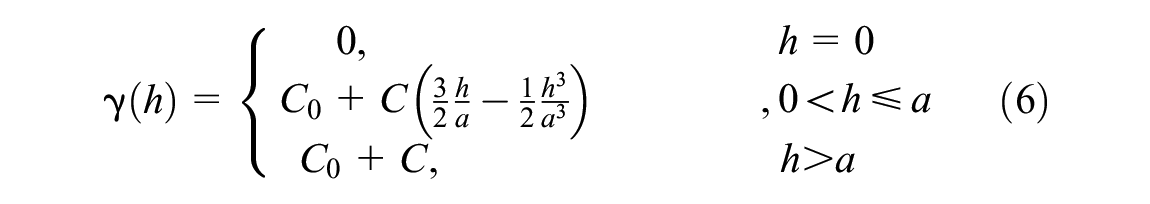
where
In addition, the Kriging method can only be applied when the stationary assumption (Equation 7) is fulfilled. The primary idea for the stationary assumption is that all the values collected at the inspection points follow the same distribution:
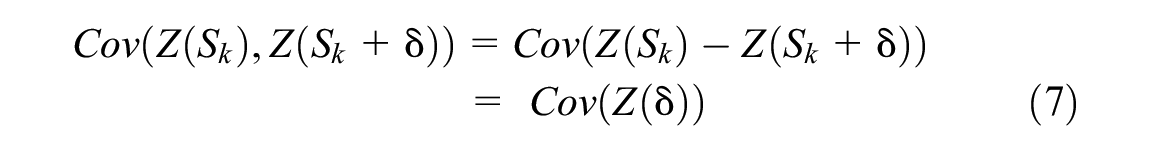
Therefore, the correlation between different inspection points can be simply demonstrated as the function of distance (time/MGT). Notice that in this study, we assume that the TQI value of a unit track corridor (100 m long according to practical usage) will follow the same distribution at a different time/cumulative MGT.
Kalman Filter Model
The KF model ( 20 ) is an optimal recursive data processing algorithm, which is applied to estimate process states based on linear systems in state space format. The general equation is addressed below:


where
Based on the model and the practical noisy data


The result is optimal when the Kalman gain matrix
Prediction Accuracy
This study applied the root mean square error (RMSE) to compare the performance of the models’ prediction results (Equation 17):
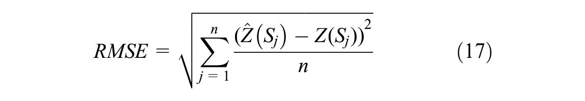
where
Case Studies
From the literature review, multiple track status degradation models are proposed, while they were rarely applied with low-quality, high-frequency, and irregularly sampled OBM data. Therefore, we perform two case studies to understand different models’ performances on hypothetical and real OBM datasets.
Case I: Model Analysis Based on Hypothetical Data
For Case I, we compare the LR, Markov, Kriging, and KF models based on hypothetical linear degraded TQI data (40 samples, following y = 0.05x) with a hypothetical threshold (y = 1). Seven different sets of data are applied, as follows.
Dataset A (linear distributed sample): sample frequency one per timestep.
Dataset B (frequency reduced sample): sample frequency one per four timesteps.
Dataset C (unbalanced sample I): where 35 samples are recorded below the threshold and five are recorded above the threshold.
Dataset D (unbalanced sample II): where 20 samples are recorded within time intervals 0–10 and 20 samples are recorded within time intervals 30–40.
Dataset E (unbalanced sample III): where all samples are recorded within time intervals 10–30.
Dataset F (uniform sample with high data error): where samples correspond to the same samples from Dataset A plus an error following N(0,0.2).
Dataset G (uniform reduced samples with high data error): where samples correspond to the same samples from Dataset A plus an error following N(0,0.2).
The first case is meant to analyze the characteristics of the proposed models considering the data frequency, data error, and data collection pattern, which are the main difficulties faced when dealing with OBM data. Notice that the Markov model applied here only has two states. As for Case II, we fit the proposed models based on the practical OBM data and TRV data to compare the models’ prediction results. Both datasets are collected from four track segments (100 m each), which have different degradation rates (T1–T4, high to low), in the western region of Switzerland. The target track geometry for the models is the longitudinal level, while the target TQI is the standard deviation of longitudinal level over 100 m. The timestep T applied for the Markov model is 8, while T applied in the KF model is (1,4,0.1,0.1,0.1,1) for dataset (A,B,C,D,E,F). In addition, the rest of the parameters used in the KF model are summarized in Equation 18:
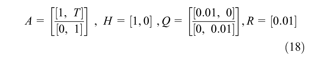
Notice that regularly sampled data is required for applying the KF model. Therefore, in Cases I and II, we preprocess the data by first dividing the time region based on the applied timesteps and then assigning the original value to the nearest timesteps.
The results for Case I are summarized in Figure 1. In Figure 1, the x-axis indicates the time, while the y-axis indicates the hypothetical TQI value. The red lines indicate the model’s prediction errors (95% confidence interval), the black dots indicate the sampled data, and the blue lines indicate the prediction results. Notice that in Figure 1, for the Markov model, we define two states for Case I, which are “above threshold” (orange) and “under threshold” (blue). Moreover, we assume that the result of the state prediction is the one with a larger probability. In Figure 1, several conclusions can be drawn from the Kriging model’s result. Firstly, we find that it can predict the degradation trend with a relatively small amount of prediction error (the confidence bound is small and close to raw data) when considering datasets A, B, C, and E. Secondly, by comparing the results generated from datasets A and B, we find that the prediction error increases by an average of 37.1% when the number of samples decreases from 40 to 10. This result proves the advantage of having more monitoring samples, as they could potentially increase the prediction accuracy. Thirdly, looking through the results generated using datasets C–E, we find that the prediction error will vastly increase when fewer samples are recorded. For example, the result obtained from applying dataset D indicates that the prediction error is increased by almost five times more than the prediction error obtained from applying dataset A. Fourthly, from the results obtained from dataset F, we find that the Kriging model’s prediction result tends to smooth out the curve compared with the fitted raw data. This indicates that the Kriging model can potentially remove a certain amount of error when used for prediction.
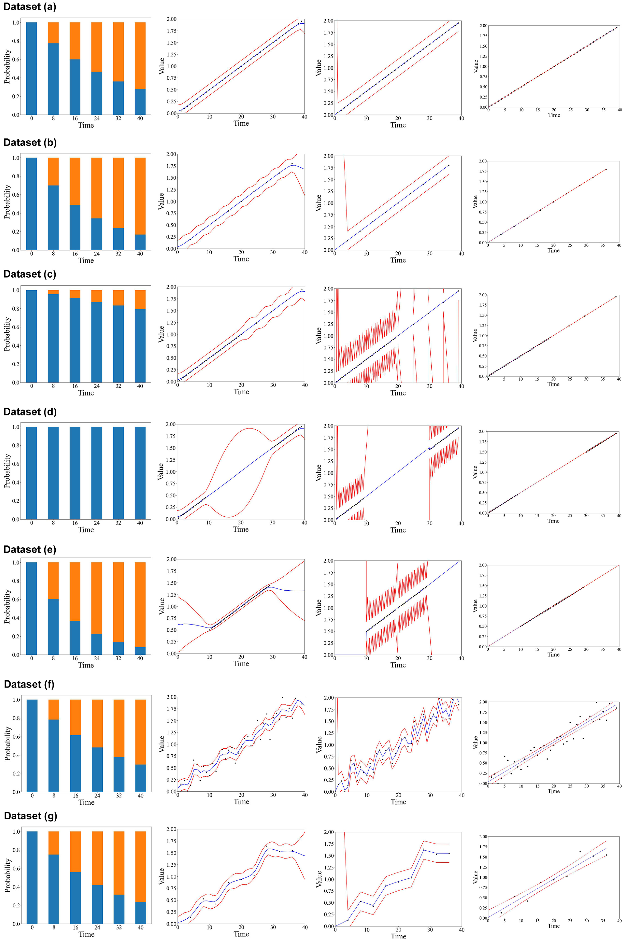
Results of the analysis based on hypothetical data. (Color online only.)
On the other hand, for the KF model’s result, we first find out that it can also predict the degradation trend with a relatively small amount of prediction error when applying datasets A and B. However, the prediction error significantly increases when no observations (monitoring points) are used. Secondly, by comparing the results generated from datasets A and B, we find that the prediction error does not significantly increase (0.03%) when the number of samples decreases from 40 to 10. Moreover, by comparing the prediction error generated from fitting datasets A–E, we find that the prediction error will be small and similar when there are observations available for update. Thirdly, looking through the results generated using datasets C–E, we find that the prediction error will vastly increase when fewer samples are recorded. Fourthly, from the result obtained from dataset F, we find that the KF model’s prediction result only slightly smooths out the curve compared with the fitted raw data. This indicates that the model’s ability to remove data errors when predicting is limited.
As for the Markov model, we first find that it predicts well when applying datasets A, B, E, and F with accuracies (number of correct predictions over the total number of predictions) of 100%, 80%, 80%, and 100%, respectively. However, it does not perform well when dealing with unbalanced samples (both datasets C and D have an accuracy of only 40%). Secondly, comparing the prediction accuracy of datasets A and B, we find that the model’s prediction accuracy decreases when reducing samples from 40 to 10. Thirdly, based on the prediction result generated by dataset C, we find that the models tend to underestimate the degradation rate when more samples are recorded in state 1 (under the threshold). Fourthly, we find that the model’s prediction accuracy is still relatively high when dealing with high sensor error dataset F. This indicates that the Markov model can withstand a certain level of low-quality data.
Last but not least, all models, except the LR model, perform poorly when no monitoring data is available in dataset D. In addition, the results obtained from datasets A, B, F, and G indicate that even with a high data error, the prediction accuracy for all models, except the Markov model, increases when the number of samples increases.
Case II: Model Analysis Based on Practical TRV and OBM Data
In Case II, we apply the practical OBM data (collected in 2019, 201 data points) and TRV data (collected from 2017 to 2019, 21 data points) to compare the models’ prediction accuracy. Firstly, we selected the data recorded before tamping (which occurred in September 2019) for fitting the models. Later on, we used the TRV data collected after tamping as the ground truth for prediction. Notice that the time period for collecting the TRV data is longer than that for collecting the OBM data to increase the number of data points for fitting the models.
In addition, for the Markov model in Case II, our target is to predict the state transfer between two inspection points where no maintenance occurs. The states are defined based on a practical regulation (EN 13848-5, 2008). The proposed Markov model contains four states, including State 1, where TQI is less than 50% of the IL threshold; State 2, where TQI is larger than 50% of the IL threshold but less than 100% of the IL threshold; State 3, where TQI is larger than the IL threshold but less than the IAL threshold; and State 4, where TQI is larger than the IAL threshold. The model’s structure is demonstrated in Figure 2, where a circle indicates a state while an arc indicates the transfer of the states.
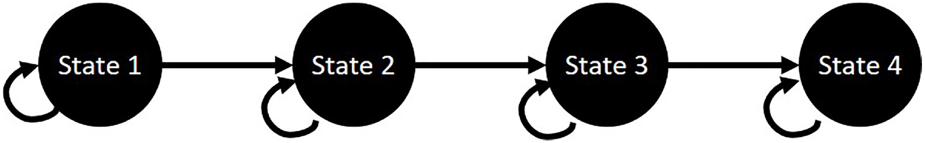
The structure of the Markov prediction model.
In addition, this study applied the RMSE to quantify the models’ prediction accuracy. For the Markov model, assume that we applied timestep T for fitting the model. Then the prediction value at a certain time t, which lies between two consecutive timesteps
The timesteps T used in Case II for the Markov model are 28 (OBM) and 140 (TRV), while those used in the KF models are 1.5 and 5. The rest of the parameters applied in the KF model are summarized in Equation 19 and determined based on practical data:

The results of Case II are summarized in Figure 3 and Table 1. In Figure 3, a–c , the red color lines indicate the results using TRV data, while the blue colors indicate the results using OBM data. The dotted lines are the 95% confidence region, and the continuous lines are the prediction results. The black dots indicate the data used for fitting the models. As for Figure 3d, the color represents the probability of the analyzed track segment staying in certain states. This includes blue indicating staying in State 1; orange indicating staying in State 2; green indicating staying in State 3; and red indicating staying in State 4. In Figure 3e, we summarize the raw data used for fitting the models, in which TRV data is red and OBM data is blue.
The Corresponding Root Mean Square Error Values for Different Models Predicting Future Track Status at Different Tracks
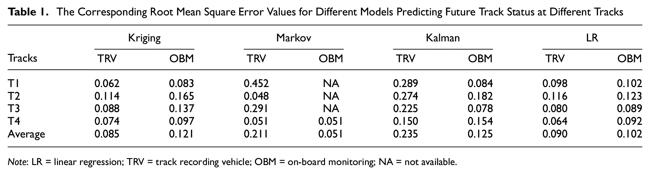
Note: LR = linear regression; TRV = track recording vehicle; OBM = on-board monitoring; NA = not available.
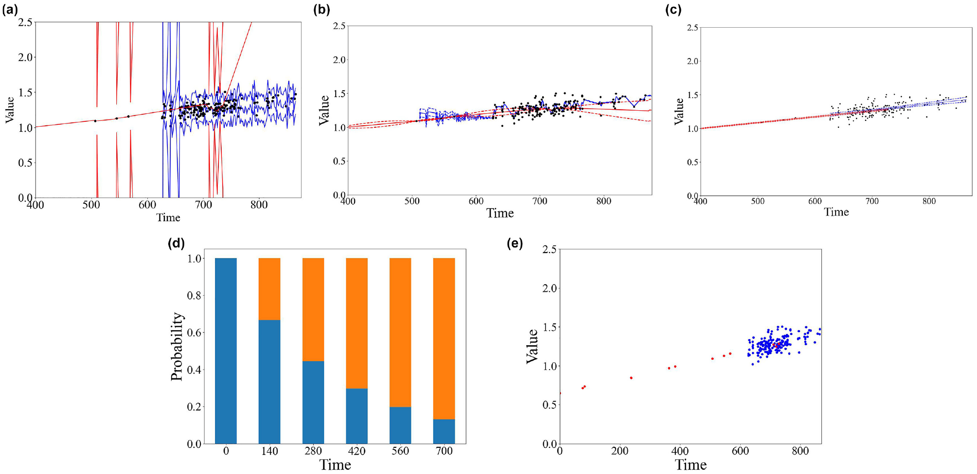
Models’ fitting results based on practical data for each model at one of the analyzed track segments: (a) Kalman, (b) Kriging, (c) linear regression, (d) Markov (track recording vehicle), and (e) raw data. (Color online only.)
Several conclusions can be observed from Figure 3. Firstly, we find out that OBM data’s variance and frequency are both larger in comparison to those of the TRV data. Secondly, despite the OBM dataset’s high variance, the predicted degradation rate is similar when applying the KF, the Kriging, and the LR models. Thirdly, the KF model, Markov model, and LR model all proposed a similar linear prediction model when monitoring data are available. However, when the monitoring points (fitting using the TRV dataset) are not available, they perform quite differently. From the results in Figure 3, the Kriging model predicts that the TQI will recover with the prediction error being increased. The LR model predicts that the TQI will increase with the same degradation rate, while the prediction error only slightly increases. The KF model predicts that both the TQI value and the related prediction error increased significantly. Fourthly, the Markov model predicted that the TQI would exceed half of the IL after 280 days, which is true since all recorded data recorded after 280 days stay in State 1. However, it also predicts that the TQI will be in State 2 forever, mainly because no data are collected in States 3 and 4. Notice that the Markov models developed based on OBM data are not shown in Figure 3. This is because the model is not formulated because of the lack of monitoring data in State 1.
After formulating the models, we applied the TRV dataset recorded after tamping as the ground truth to estimate the prediction accuracy (RMSE) of the models. The models are translated to the first monitoring point, which is set as the origin. The results are summarized in Table 1. The average prediction accuracies for the TRV dataset from high to low are Kriging > LR > Markov > KF, while for the OBM dataset they are Markov > LR > Kriging > KF. Moreover, the Kriging model tends to perform slightly better than the LR model when dealing with tracks with higher degradation rates (T1, T2), while the KF model sometimes performs better than the LR model when applying OBM data (T1, T3). For the Kriging model, we observe that it performs slightly better when applying TRV data. As for the KF model, it performs better when applying the OBM dataset. The Markov model’s RMSE values vary from case to case, which indicates the model is unstable. Moreover, if we apply the accuracy used in Case I, the results are (62.5%, 100%, 100%, 100%), which is quite good on average. The LR model performance for both datasets is quite similar.
Discussion
In this research, we aim to assist railway operators in using OBM data to predict future track status. The literature review discusses multiple track status degradation models previously applied and their characteristics related to data usage. Four models are later proposed for examination and comparison. The goals are to understand the models’ characteristics when dealing with irregular sampling, sampling frequency, and data error and, moreover, to understand whether commonly used models (LR and Markov) and the newly proposed models (Kriging and KF) can be applied to TRV data and OBM data or not.
For the LR model, which is the most commonly used track degradation model, the resulting analysis shows that it can be easily applied to irregular sampling. The model can also be applied to high-frequency data, where the prediction accuracy may increase as the monitoring frequency increases. When dealing with data with larger errors, the models tend to generate results with a higher RMSE, while the RMSE value is still lower than other proposed models. The major limitation of the LR model is that it is unable to predict nonlinear degradation rates. As stated in Table 1, a track with higher degradation rates tends to degrade nonlinearly, which results in the model having a higher RMSE compared to the Kriging model’s RMSE at tracks T1 and T2. When applying models to the OBM and TRV data, we find that the RMSE values are similar, while the RMSE value from OBM data is slightly larger than that from TRV data. This indicates that the model can be applied using both datasets with similar prediction accuracy.
As for the Markov model, the result shows that it is strongly affected by irregular and unbalanced sampling. This is because the formulation of the cumulative distribution function (CDF) is closely related to the timestep that is used for prediction. When the prediction timestep used for prediction is less than the minimum interval between recorded monitoring points, those samples will be neglected when formulating the cumulative distribution. This eventually results in reducing the accuracy of the prediction. One can improve this process by fitting the discrete CDF with continuous CDF. However, the unbalanced recorded samples will make the proposed CDF biased. For example, in the result obtained in dataset C, most of the samples are collected within State 1 (under the threshold). This eventually results in overestimating the probability of samples staying in State 1 for each timestep and underestimating the degradation process. This type of problem has not been widely discussed by the literature that applied the Markov model for prediction, because the previous studies usually applied data recorded by inspection trains. This type of data is usually periodically recorded two to three times per year, which enables one to assume that all data are recorded uniformly. However, for OBM data, this is usually not the case. In addition, the prediction accuracy of the Markov model is not sensitive to the monitoring frequency and the data error compared to other models. In fact, the number of samples distributed in each state, whether they are distributed uniformly or not, and the size of the states are the factors that significantly affect the model’s prediction result. To sum up, we suggest applying this model with datasets that are periodically collected. The model can also be applied to low-quality data since it can withstand a certain amount of data error. As for determining the state setting of the model, one should consider the distribution of the monitoring points before formulating the model.
The Kriging model performs similarly to the LR models. It can be applied using irregularly and unbalanced samples, while the prediction error significantly increases if no monitoring point is recorded with a long time interval. Unlike the LR models, the Kriging model can better demonstrate nonlinear degradation. It can also smooth the prediction curve, removing a certain amount of data error. However, the Kriging model can be easily affected by extreme values (high data error) since it firmly believes in the monitoring point values. The prediction will become even more biased if no samples are available. Take the results obtained from datasets F and G as an example. The prediction accuracy reduces significantly when samples are removed. Since the number of samples would significantly affect the result for the Kriging model and the high-frequency data can reduce the prediction error, we suggest applying this model using OBM data.
The KF model is commonly applied by using periodic monitoring data since it predicts and updates its prediction by uniform timesteps. In this study, we preprocess the distance between each applied data into multiple timesteps to create the periodically sampled data. The timestep is set small enough to not significantly affect the data. However, the small timestep will result in the model predicting multiple times without an update from monitoring points, which significantly increases the prediction error. Therefore, we strongly suggest applying periodic monitoring data when applying this model. The KF model can predict the linear and nonlinear degradation processes with relatively small prediction errors by receiving a periodic monitoring dataset. On the other hand, the KF model, similar to the Kriging model, is strongly affected by the frequency of sampling. The prediction error will significantly increase when no data points are updated. Therefore, we suggest applying this model using OBM data.
As a result, all four proposed models can be applied by using OBM data. The LR model can provide the most stable and accurate prediction result when the track is assumed to be degraded linearly. When dealing with a heavily loaded or old track, in which the degradation process tends to perform nonlinearly, the Kriging and the KF models can better predict the result. In addition, the KF model performs better when the data is sampled periodically, while both of them require a high-frequency dataset for better prediction. As for the Markov model, it can apply data with lower frequency and data quality. It can also demonstrate a nonlinear degradation rate. The major limitation of the Markov model is that it is strongly affected by the sampling distribution, which may require filters being applied before applying OBM datasets
Conclusion
This study reviews various track status degradation models and proposes several models for examination and comparison to understand the models’ characteristics and performance when dealing with different datasets. The goals are to assist railway operators in using OBM data for predicting future track status. By understanding the degradation models’ characteristics, railway operators can efficiently predict the future track status, which is useful in scheduling maintenance and inspections. The ultimate goal is to attain a lower life cycle cost at the system level while safety and availability are guaranteed.
The literature review shows the application of OBM data for prediction has received more and more attention in academia so far. We argue that the OBM data have higher data collecting frequencies and sensor errors compared to traditionally used TRV data, which requires new models for application. The commonly used model performance on the new dataset should also be considered and analyzed.
The study proposes four models (i.e., the LR model, Markov process model, ordinary Kriging model, and KF model) for predicting future track status based on the application of hypothetical, TRV, and OBM data. The results show that the LR models can withstand irregular sampling and provide the most stable and accurate prediction result when the track status degrades linearly. The Kriging and KF models can better predict the result when the track status degrades nonlinearly, while the prediction accuracy would increase when more samples are available. The Markov and KF models are more likely to be affected by irregular sampling because of their model formulations, whereas the Markov model’s prediction accuracy would be strongly affected by the sample distribution rather than sample frequency.
To sum up, we suggest railway operators apply the LR model for applying OBM data and specifically apply the Kalman or the Kriging model at places (highly loaded or old track) that are most likely to degrade nonlinearly. The Markov model can be applied when the data quality is relatively low, while the state setting of the model should further consider the sampling instances. The analysis of the characteristics of different possible machine learning approaches (for example, the difference between the k-nearest neighbor, the linear model, decision trees, and the neural network) will be a future step for this study.
Footnotes
Author Contributions
The authors confirm their contribution to the paper as follows: study conception and design: T.H. Yan, M.A. Costa, F. Corman; data collection: T.H. Yan; analysis and interpretation of results: T.H. Yan, M.A. Costa, F. Corman; draft manuscript preparation: T.H. Yan, M.A. Costa, F. Corman. All authors reviewed the results and approved the final version of the manuscript.
Declaration of Conflicting Interests
The author(s) declared no potential conflicts of interest with respect to the research, authorship, and/or publication of this article.
Funding
The author(s) disclosed receipt of the following financial support for the research, authorship, and/or publication of this article: This research was supported by a grant (project OMISM) from the ETH Zurich Mobility Initiative and a Swiss Government Excellence Scholarship (grant No. 2021.0152).