Sage Journals: Discover world-class research

Abstract

This research investigates the effectiveness of several strategies to deploy roadway maintenance machines (RMMs) in preparation for overnight maintenance in rapid transit systems. Owing to the short windows of time available for maintenance activities in the overnight period (i.e., when revenue service is suspended), efficient deployment of RMMs is an important aspect of ensuring adequate productive time for crews at work locations. Four deployment strategies are investigated: optimizing the long-term yard storage locations of RMMs; optimizing the assignment of RMMs to work zones; optimizing the use of nonrevenue locations within the network to “preposition” RMMs closer to their work zones; and optimizing the routing and scheduling of RMMs through the network to reach the work zones. The strategies have been tested using data from the Washington Metropolitan Area Transit Authority. The results indicated that the proposed strategies reduced the time needed for RMM deployment. In the case of prepositioning, the median prepositioned RMM was deployed 23 min earlier than in the baseline (i.e., routing and scheduling alone) scenario, and the median RMM receiving a new yard storage location was deployed 16 min earlier. This was achieved without widespread negative impacts to RMMs that could not benefit from the proposed strategies for operational reasons. The results also demonstrated the potential of the routing and scheduling model as a tool to evaluate the deployment time impacts of distance-minimizing strategies, considering factors such as conflicts between RMMs and the availability of tracks to avoid disruptions to revenue service.

Keywords

public transportation maintenance management heavy rail management operation

Urban rail systems require regular maintenance to remain in good operating condition. Although some maintenance activities (for example, visual inspection) can be performed under traffic, other maintenance activities can only be performed when revenue service along the affected right-of-way is suspended. Examples include rail or tie replacement, major structural repairs, or power system maintenance. Given the lower travel demand during nighttime, many urban rail operators use an overnight period during which limited or no revenue service is provided and maintenance activities can be prioritized.

However, this daily overnight period of revenue service suspension can be short, and there are several operations that must be completed in this period to facilitate the handover from revenue operations to maintenance activities. This includes returning revenue trains to yards, deploying crews and/or equipment (both on foot and via several varieties of “RMMs,” or roadway maintenance machines), and deenergizing the power system for worker safety. Most of these operations must then be repeated in reverse at the end of the night to facilitate the handover from maintenance activities back to revenue operations, as shown in the timeline in Figure 1. To capitalize on overnight work windows, it is critical for urban rail operators to practice these handover and preparation activities as efficiently as possible. Efficient handovers help crews and maintenance managers maximize “wrench time”—the time spent on productive maintenance tasks (e.g., replacing a section of rail).

Figure 1.

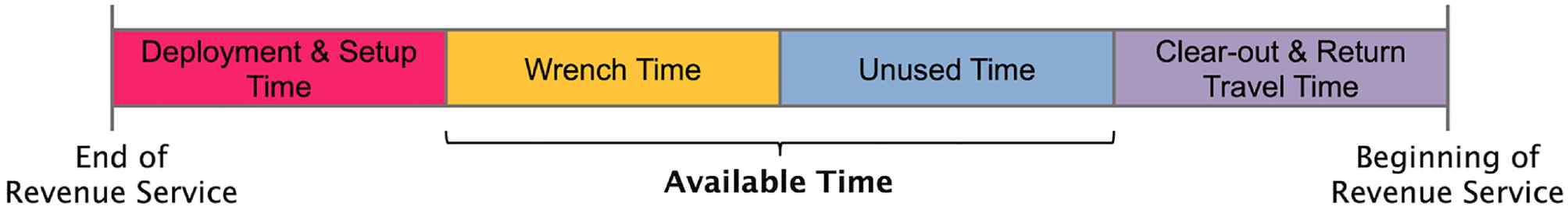
High-level timeline of an roadway maintenance machine + crew in the overnight maintenance window.

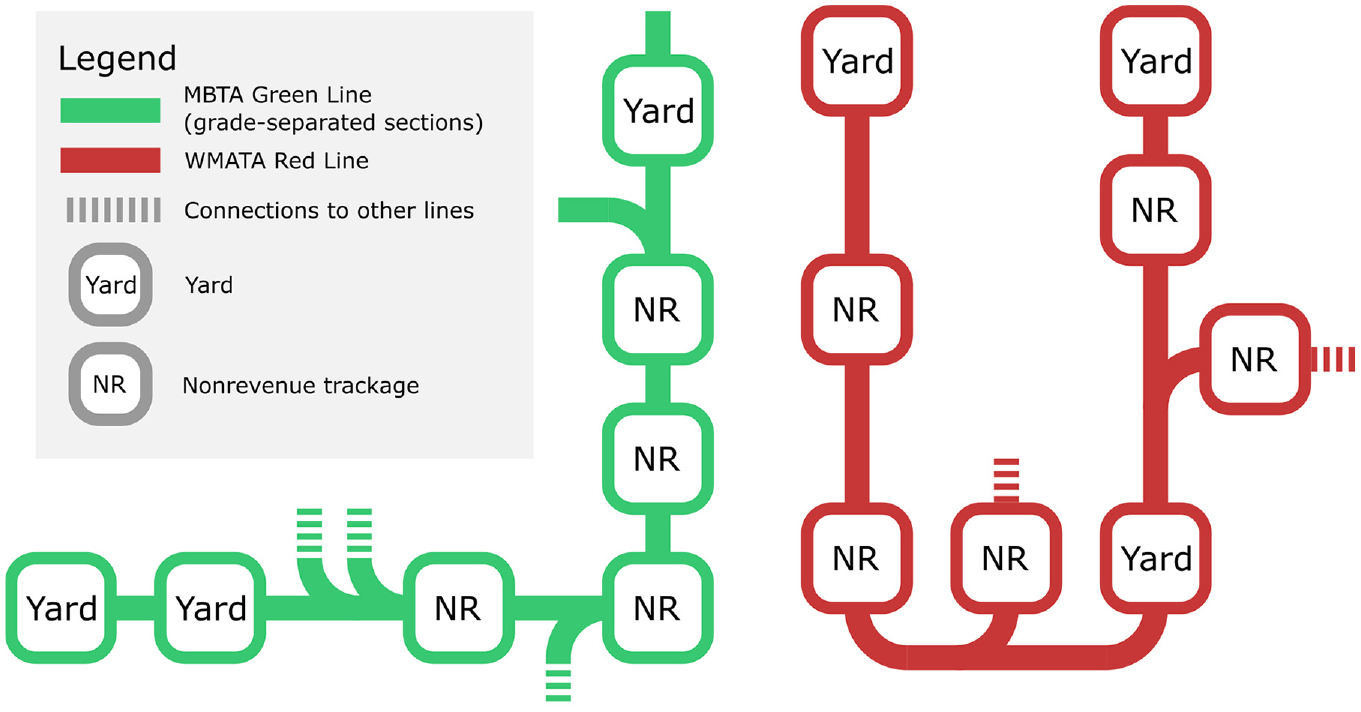
This research investigates strategies to improve the efficiency of one of these handover activities: the deployment of RMMs throughout the network. Although the physical deployment of RMMs typically occurs on the same night of work (with RMMs departing yards shortly before or after the end of scheduled revenue service), the planning for RMM deployment starts years in advance of the actual work with the procurement of RMMs, as the pool of available RMMs influences later decisions such as the assignment of RMMs to work zones. Table 1 describes the various stages of planning for RMM deployment in the order that they would generally occur at a transit agency.

Table 1.

RMM Deployment Planning Stages

Planning stage	Description
Determining long-term storage locations of RMMs	Allocating space at rail yards to facilitate the storage of RMMs, including the staging of crews, materials, and equipment
Assignment of RMMs to work zones	Given a work zone that requires an RMM, determining which RMM (and, by extension, which yard) will serve the work zone
Operations planning	Given revenue service patterns and RMM origins and destinations, determining the routing of RMMs, the scheduling/timing of RMM departures from yards, and whether to send RMMs directly to the work zone or to stage temporarily within the network along the way
Deployment	Safely moving the RMMs through the network according to the operations plan

Note: RMMs = roadway maintenance machines.

The complexity of planning tends to increase as the complexity and inaccessibility of the network increases. For example, a transit system without any connections between lines, each line possessing a singular yard (e.g., the Massachusetts Bay Transportation Authority’s [MBTA] Red, Orange, and Blue Lines [ 1 ]), would have a simplified assignment of RMMs to work zones: work being done on any line must be served by an RMM coming from that line’s yard. San Francisco Municipal Transportation Agency’s Muni Metro has a large and interconnected network; however, only 9 of its 120 stations are located within tunnels ( 2 ), and the rest of the network is at-grade and readily accessible by rubber-tired vehicles traveling on public streets. Therefore, the RMM deployment problem is also simplified by the increased number of access points.

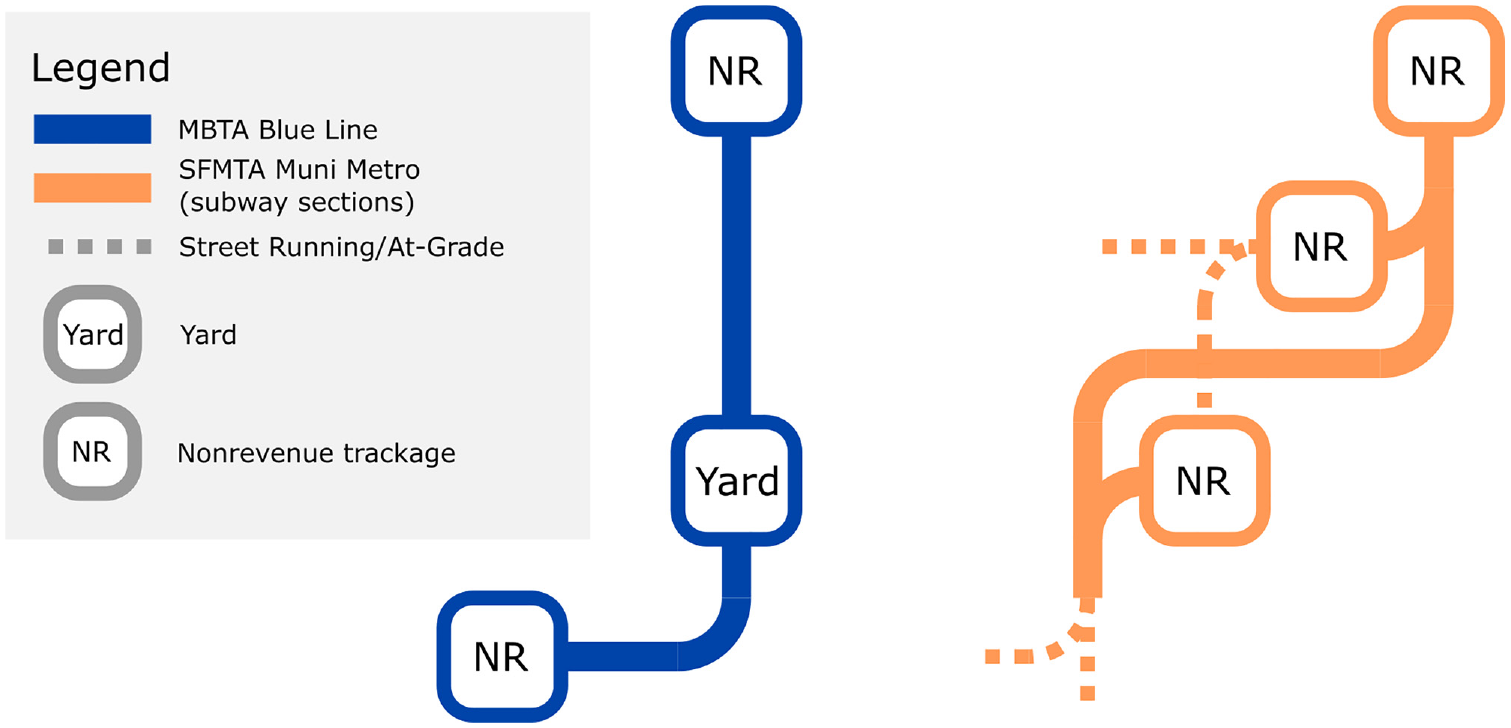
However, for many transit networks this is not the case. For example, despite being a light rail system, a large portion of MBTA’s Green Line network is grade-separated without easy access from public streets, and this portion contains three yard facilities and four locations with trackage that is rarely used for revenue service ( 1 ). Washington Metropolitan Area Transit Authority’s (WMATA) fully interconnected network contains, in total, 9 yards and 14 locations with nonrevenue trackage, with several track connections between lines ( 3 ). In networks like these, decisions such as the yard storage locations of RMMs, assignment of RMMs to work zones, and routing become more complex; however, there are also greater opportunities for efficient deployment strategies.

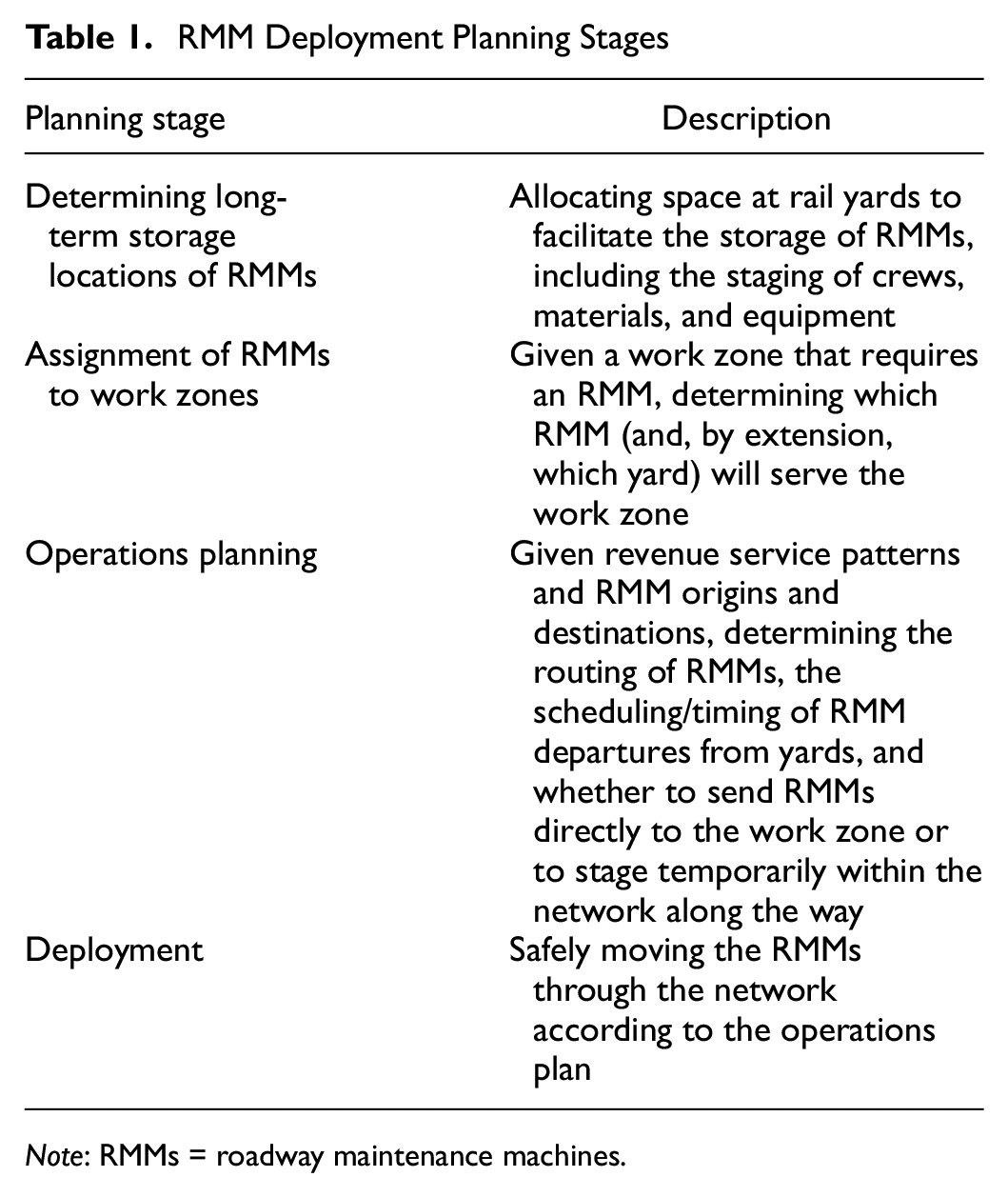
To compare these network topologies at a high level, Figure 2 shows two examples of lines/systems with lesser potential for efficiency improvements in RMM deployment. On the other hand, Figure 3 shows two examples of lines/systems with greater potential for efficiency improvements in RMM deployment. Note that WMATA’s Red Line can also be served by RMMs coming from the rest of WMATA’s system via track connections to other lines, increasing the complexity of the problem further (and providing more potential for efficiency gains).

Figure 2.

Examples of lines with lesser RMM deployment improvement potential: MBTA Blue Line and SFMTA Muni Metro (subway sections).

Figure 3.

Examples of lines with higher RMM deployment improvement potential: MBTA Green Line and WMATA Red Line.

Literature Review

RMM deployment can be generally described as a combination of several types of problems. This paper will focus on the problem of resource allocation (e.g., the allocation of yard space to RMMs, the assignment of RMMs to work zones, and the allocation of space in the network to RMMs being deployed) and the problem of routing (i.e., efficient movement of RMMs through the network). There has been little research on the application of these problems to RMM deployment for urban rail networks, but similar problems can be found in the literature.

Optimal resource allocation strategies appear in several contexts within mass transit, for example, in the allocation of buses to deal with unexpected rail disruptions ( 4 ) or in frequency setting problems to allow for sufficient social distancing aboard rail vehicles ( 5 ). Although research exists into the optimization of resource allocation for maintenance-related problems in the mass transit context, these generally focus on vehicle/fleet maintenance ( 6 , 7 ). Similar decisions are present in the rail maintenance problem and in the vehicle maintenance problem (e.g., allocation of yard space to vehicle maintenance, assignment of vehicles requiring maintenance to maintenance facilities), but the vehicle maintenance problem typically does not assign precedence to these decisions as they do not have as large an impact on the overall availability of vehicles. However, in the urban rail maintenance problem, these decisions can have a major impact on the available time for maintenance work in the short overnight windows.

In other contexts, RMMs are also a component of scheduling problems (e.g., scheduling work events to enable efficient RMM deployment) ( 8 , 9 ). This is mission-critical in national rail networks, where “repositioning costs” (the costs of moving RMMs from one work zone to another) are measured in days ( 10 ). Several of the proposed strategies for improving RMM deployment involve similar reduction of repositioning costs in the form of minimizing the distances traveled by RMMs in the post-revenue period. However, unlike in national rail networks, the shorter distances involved in urban rail networks means that RMM travel distances are often not a consideration when scheduling work events. Therefore, although this scheduling problem will be considered in future research, it is assumed in the context of this paper that work events are scheduled independently of the RMM deployment and are inputs to the process.

Finally, the routing and scheduling of yard departures of RMMs will also be investigated in this paper. Although complex urban rail networks such as those in New York City ( 11 ) or London ( 12 ) may allow for complex routing options for passenger services, most urban rail systems are designed for lines to be operated with limited interaction with other lines. Therefore, questions of scheduling for urban rail networks often focus on line-by-line timetabling (with an objective of reducing passenger wait times or transfers), and routing is rarely considered. However, there are limited examples of optimal routing strategies being applied to urban rail networks: for example, in the formation of dynamic routes in Hong Kong’s flexible light rail transit network ( 13 ), in the routing of passengers in the Last Train Timetabling Problem ( 14 ), and in the routing of deadheading trains to begin service in the morning ( 15 ). However, the problem of RMM routing and scheduling requires a more detailed model of the network, as directional running on tracks is not necessary, track crossovers can be used to avoid crossing other work zones en route, and the primary way in which time penalties are incurred is through conflicts with other vehicles. Therefore, a new method of optimizing routes and schedules over the rail network has been developed for this purpose that takes into consideration these factors.

Problem Statement

Given the unique requirements of overnight maintenance of urban rail systems, this research investigates various strategies to improve the deployment of RMMs:

Yard storage location: optimizing the long-term storage locations of RMMs (i.e., the yards at which they will be stored and most often be departing from) to minimize the overall distance to travel to work zones. Optimal yard storage locations are based on an expectation of the locations of work zones that will be served in the future.

Assignment: optimizing the night-by-night assignment of RMMs to work zones, considering the specific type of RMM that is required by the work zone and the availability of RMMs at yards. Although it is a similar objective to the yard storage location problem, assignment assumes fixed RMM availability at yards and definite work zone locations for short-term planning.

Prepositioning: optimizing the night-by-night decision to “preposition” RMMs within the network, which involves moving RMMs during revenue service to nonrevenue tracks within the network close to the end of revenue service to position them closer to their work zones (thus minimizing the post-revenue-period distance to travel).

Routing and scheduling: optimizing the routing of RMMs through the network and the scheduling of yard departures and other movements, given the location of each RMM at the end of revenue service and the locations of the work zones they will serve.

To suit the diverse operational needs of transit agencies, these strategies can be applied separately or together to improve the efficiency of RMM deployment. Different planning horizons, network topologies, and organizational responsibilities may render certain strategies more appropriate than others depending on the agency. Table 2 lists the four strategies alongside their planning horizons and appropriate system/network configurations.

Table 2.

RMM Deployment Strategies

Strategy name	Planning horizon	Appropriate system/network configuration
Yard storage location	Yearly or longer	Yards serving multiple lines, track connections between lines, groups of interoperable RMMs, flexibility in usage of yard facilities
Assignment	Weekly or daily (depending on additional preparation time needed)	Yards serving multiple lines, track connections between lines, groups of interoperable RMMs, availability of pre-deployment crew transport (e.g., crew shuttles)
Prepositioning	Weekly or daily (depending on additional preparation time needed)	Nonrevenue trackage, e.g., pocket tracks, tail tracks, sidings; crew schedules that allow yard departures earlier than end of revenue service; guidelines for mixed-traffic operations between revenue vehicles and RMMs
Routing and scheduling	Daily: real-time	Complex networks, crossovers, track connections between lines

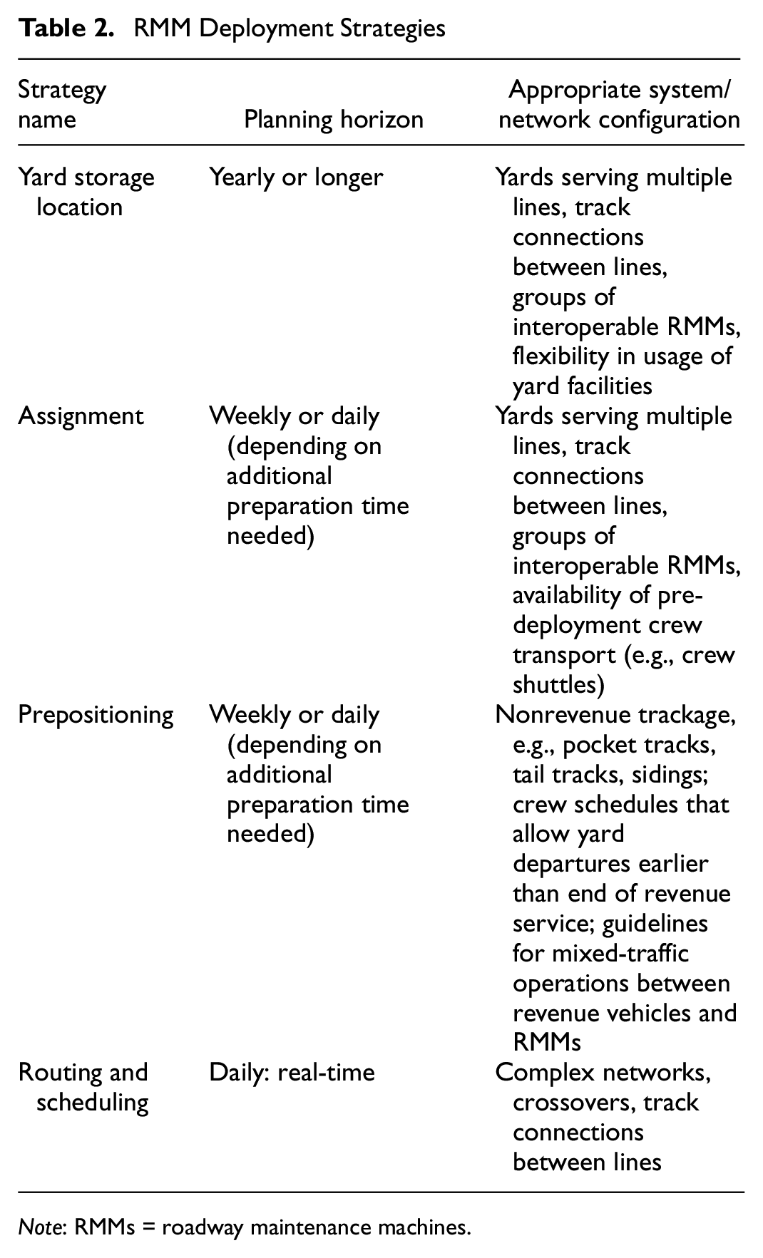
Note: RMMs = roadway maintenance machines.

The main contributions of this research are,

Identification of RMM deployment strategies appropriate for the urban rail system context;

Formulation of the various strategies as optimization problems, using commonly available data sources as inputs and constraints to reflect realistic operational considerations, with the aim of creating useful decision support tools; and

Demonstration and analysis of the potential benefits of the various strategies through a case study using real-world data from WMATA.

The paper is laid out as follows: first, the various RMM deployment strategies are described at a high level, outlining the objective, inputs, and considerations. Next, contextual background about a case study at WMATA is provided. Then, the results of the various strategies are shown and compared with one another as well as to a baseline based on real-life deployment plans.

Methodology

The strategies investigated in this paper are formulated as mixed-integer optimization problems. The first three strategies (yard storage location, assignment, and prepositioning) aim to minimize the post-revenue-period distance traveled between the yard (or prepositioning location) and the work zone across all RMMs. The last strategy (routing and scheduling) aims to minimize the “setup ready time” across all crews: specifically, the earliest time at which a crew is both a) at its work zone, and b) no longer waiting for any other RMMs to cross its path.

Although the strategies can be implemented as standalone decision support tools, they are not mutually exclusive. For example, the prepositioning model takes, as an input, the yard-to-work zone RMM assignments for a given night. These yard-to-work-zone RMM assignments could be generated from the assignment model. The routing and scheduling model also takes as an input the yard-to-work zone assignments, but can also take into account the prepositioned locations of RMMs if applicable. In this way, the strategies can build on each other.

In the following subsections, the models underlying each strategy will be described in more detail: specifically, the objective, the options considered by the model, inputs, and operational considerations.

Yard Storage Location

The yard storage location strategy aims to minimize the expected distance traveled to the work zone across all RMMs by optimizing the long-term storage locations of RMMs within yards. The model can be based on historical data (which assumes that the spatial distribution of work zones over the rail network in one time period will be representative of a future time period), or, if planning horizons are sufficiently long and stable, the model can use planned work zones to recommend the yard storage locations of RMMs.

If data are available, the capacity of each yard to store RMMs can be limited by the number of spaces required for out-of-service RMMs undergoing maintenance, or limited to specific types of RMMs that the yard can support (e.g., because of equipment, materials, or labor staging considerations). Furthermore, the type of RMM required to serve a work zone can be constrained to specific vehicles, groups of similar RMMs owned by the same organization, or groups of similar RMMs owned by any organization, based on the level of interoperability between similar RMMs.

The yard storage location model is formulated as a mixed-integer optimization problem with linear constraints, with the following decision variables:

$x_{j}^{g} \in Z \geq 0 : number of RMMs of group g stored at yard j$

$w_{jk}^{gn} = {\begin{matrix} 1, & if an RMM in group g on night n leaves yard j to serve work zone k \\ 0, & otherwise \end{matrix}$

The following inputs are also considered:

C_j = RMM storage capacity of yard j

d_jk = Distance from yard j to work zone k

F_g = size of the fleet in group g

K_gn = set of all work zones on night n requiring an RMM from group g

The objective function is to minimize the distance traveled by all RMMs across all nights,

Minimize \sum_{gnjk} d_{jk} w_{jk}^{gn}

(1)

Four constraints are added: Equation 2 prevents the storage capacity of yards from being exceeded, Equation 3 ensures that all RMMs within a given group are assigned to yards, Equation 4 ensures that the number and variety of RMMs deployed from each yard and each night does not exceed what is stored, and Equation 5 ensures that every work zone is assigned an RMM from the necessary group.

\sum_{g} x_{j}^{g} \leq C_{j} \forall j

(2)

\sum_{j} x_{j}^{g} = F_{g} \forall g

(3)

\sum_{k} w_{jk}^{gn} \leq x_{j}^{g} \forall g, n, j

(4)

\sum_{j} w_{jk}^{gn} = 1 \forall k \in K_{gn} \forall g, n

(5)

Assignment

The assignment strategy aims to minimize the expected distance traveled to the work zone across all RMMs by optimizing the assignment of RMMs to work zones. Inputs to the problem are the locations of RMMs on the day that the deployment is being planned, the locations of work zones, and the type of RMM that is needed. Similar to the yard storage location strategy, the type of RMM can be defined more narrowly (e.g., “an RMM of the ‘prime mover’ variety owned by organization A”) or more broadly (e.g., “any prime mover”) to reflect different levels of interoperability between similar RMMs.

The assignment strategy is modeled as a typical assignment problem, which may be solved by standard network optimization methods. The problem is set up and solved separately for different groups of RMMs and for each night, as assignments within a group of RMMs and for one night are made independently of other groups and other nights. A single decision variable is required: $x_{jk}$ , the flow of RMMs along arc $jk$ (e.g., from yard $j$ to work zone $k$ ). Arcs are created for every pairing of yard-to-work zone, as well as for every yard to the sink node for unused RMMs. In addition, the following inputs are used:

S = set of yard nodes,

T = set of work zone nodes,

U = universal sink node for unused RMMs,

r_j = number of RMMs available at yard j∈S,

Q = number of unused RMMs (known in advance), and

d_jk = distance (cost) to travel across arc jk.

The objective function is to minimize the distance traveled by all RMMs in the group on the particular night:

Minimize \sum_{jk} d_{jk} x_{jk}

(6)

The four constraints for the problem are shown below. Equation 7 is a capacity constraint to ensure that no more than 1 RMM travels from any yard to a work zone. Equation 8 requires that all RMMs in a yard are either assigned to a work zone or to the unused RMM node. Equation 9 ensures that every work zone receives exactly 1 RMM. Equation 10 ensures that all unused RMMs are assigned to the unused RMM node.

x_{jk} \leq 1 \forall k \in T

(7)

\sum_{k} x_{jk} = r_{j} \forall j \in S

(8)

\sum_{j} x_{jk} = 1 \forall k \in T

(9)

\sum_{j} x_{jU} = Q

(10)

Prepositioning

The prepositioning strategy aims to minimize the expected post-revenue-service distance traveled to the work zone across all RMMs by optimizing the use of nonrevenue locations in the network by RMMs “prepositioning” closer to their work zones. Nonrevenue locations include pocket tracks, tail tracks, center tracks at stations not normally used for revenue service, and track connections between lines, among other features. Although some of these locations may be used for headway maintenance in the form of short-turning trains or gap trains, it is rarer for these measures to be employed near the end of revenue service, when passenger demand is lower and trains are returning to yards. The model takes into consideration the capacity of the individual prepositioning locations; whether the variety of RMM is capable of being prepositioned (e.g., rail trains, which carry 1,600-ft strands of continuously welded rail, cannot fit into prepositioning locations); whether a prepositioned RMM serves a work zone that would still allow other RMMs to pass (thereby enabling an earlier setup time); and control center workload, by limiting the number of RMMs that can be moved through mixed traffic in any given operational jurisdiction.

Where standard operating procedures allow for RMMs and revenue trains to operate in mixed traffic, staging RMMs in prepositioning locations shortly before the end of revenue service allows for RMMs to be closer to their work zone when the network becomes available for work zones to be set up. To demonstrate, Figure 4 shows the path of an RMM (shown as a yellow rectangle) over a generic rail network to reach a work zone on the other side of the network from its yard. This is the distance that would be traveled in the post-revenue-service period. To contrast, Figure 5 shows the path of an RMM over the same network but beginning from the pocket track closer to the work zone. It is likely that the RMM in Figure 5 will reach its destination sooner than the RMM in Figure 4 owing to the shorter travel distance.

Figure 4.

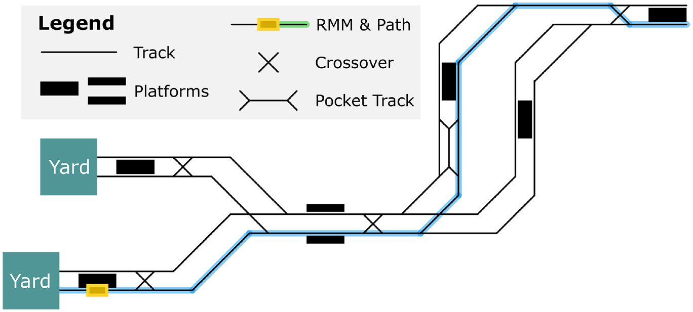
Example RMM routing on a generic network without prepositioning.

Figure 5.

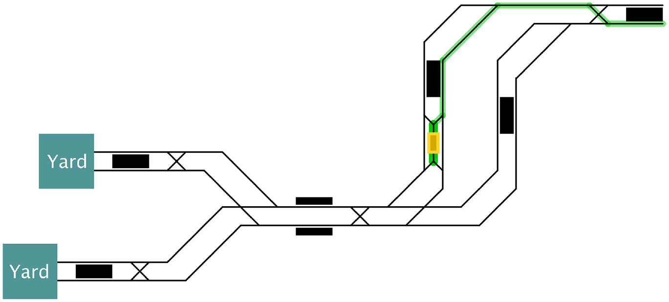
Example RMM routing on a generic network with prepositioning.

The prepositioning model is similar to the assignment model, but with the addition of nodes representing prepositioning locations, with additional arcs connecting yards to prepositioning locations and prepositioning locations to work zones. All of the variables and notation from the assignment problem are kept, and the following (nondecision) variables and inputs are added:

$P$ = set of prepositioning nodes,

$p_{i}$ = capacity of prepositioning location i, and

α = prepositioning distance weight.

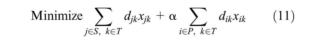
The objective function is to minimize the sum of the distance traveled by RMMs from yards to work zones, along with a weighted sum of the distance traveled by RMMs from prepositioning locations to work zones,

Minimize \sum_{j \in S, k \in T} d_{jk} x_{jk} + α \sum_{i \in P, k \in T} d_{ik} x_{ik}

(11)

In addition to the constraints in the assignment model, the following constraints are also added. Equation 12 ensures that no more than 1 RMM travels from a prepositioning location to a work zone, Equation 13 requires that all RMMs entering a prepositioning location leave to serve a work zone (i.e., conservation of flow), and Equation 14 ensures that the capacity of the prepositioning location to store RMMs is not exceeded.

x_{ik} \leq 1 \forall i \in P, k \in T

(12)

\sum_{j} x_{ji} - \sum_{k} x_{ik} = 0 \forall i \in P

(13)

\sum_{j} x_{ji} \leq p_{i} \forall i \in P

(14)

Routing and Scheduling

The routing and scheduling strategy aims to minimize the overall time at which RMMs and work zones are “setup ready.” A work zone or RMM being “setup ready” means that 1) the RMM has reached the work zone, if applicable, and 2) all other RMMs that must pass through the work zone to get to their own destinations have already done so. Within the model, RMMs may use any track(s) on the rail network to proceed from yards to work zones; however, conflicts between RMMs incur time penalties equivalent to the amount of time to pass at the nearest crossover from the point of the conflict. Furthermore, segments of track are only made available for RMM usage after the final revenue trains pass those segments (including a buffer time). Parameters are also included to add time penalties for instances of crossover usage in networks where this creates additional workload (e.g., if switches must be manually activated by rail traffic controllers). The average speed of an RMM between points of the network may not exceed a specified maximum average cruising speed.

Work zones without RMMs may be included as static points with their own setup times. In this case, the work zone has reached its “setup ready” time if all RMMs that must pass through the work zone to get to their own destinations have already done so. This encourages detouring of RMMs to avoid crossing through work zones on the network even if there is not a conflict with another RMM.

The solutions generated by the routing and scheduling model are reasonable and comparable to real-world routing and scheduling decisions at a high level. The model minimizes the sum of all “setup ready” times across all work zones, subject to the following constraints:

Each RMM is assigned one route through the network of many possible routes. Routes consist of predefined route segments.

Each RMM is assigned one path (traveling either down Track 1 or Track 2) through each route segment.

RMM travel time from one station to the next station must be greater than the minimum run time between those stations.

An RMM is not “setup ready” until it has reached the end of its route.

An RMM is not “setup ready” until all other RMMs passing its work zone have done so.

RMMs passing through stations on the same track in the same direction must be separated by a minimum headway.

RMMs passing through stations on the same track in opposite directions must be separated by a minimum length of time equal to the time it takes for the trains to maneuver around one another at the nearest crossover.

Every instance of crossover use on an RMM’s path incurs a penalty.

A track at a station does not become available for RMM travel until the final revenue train has departed from that track at that station.

Case Study

The four strategies described have been applied using real-life data from WMATA. Track schematics were used to build the underlying graph representation of the networks for the various models, and standard operating procedures as well as interviews with operations staff provided guidance on network- and movement-related input parameters.

Track circuit data showing the locations of vehicles were used to construct trajectories of RMMs, which were compared with work log data and yard tower operations data to identify the administrative and operational details of real-life RMM trips. RMM maintenance logs and yard movements were used to infer the effective capacities of yards for storage of in-service RMMs. Finally, rail schedules were compared with track circuit data to determine track availability for the purpose of routing RMMs so that there is no interference with revenue service. The analysis covered 110 work days between July 2021 and November 2021.

The WMATA network is large and complex, and all lines are fully accessible and technologically compatible from a rail movement perspective. Figure 6 shows the basic structure of the network at the line level (i.e., individual tracks and crossovers are not represented, but major features such as yards, connections between lines, and nonrevenue track locations are represented). In total, there are nine yards on the WMATA network, eight of which were in service during the analysis period. There are also 16 distinct locations with nonrevenue trackage (e.g., pocket tracks, tail tracks), 15 of which were in service during the analysis period.

Figure 6.

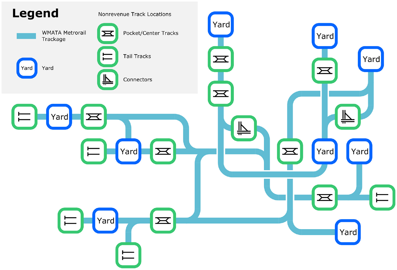
Schematic of WMATA network at the line level.

Results and Discussion

An important aspect of the proposed RMM deployment strategies is that they may be implemented individually or in sequence. For example, the routing and scheduling strategy may be evaluated using actual departure yards and work zones as its inputs to obtain the optimal routing and scheduling for these deployments, as well as the projected optimal setup ready time for each RMM (the time at which an RMM has reached its work zone and no further RMMs must cross that work zone). However, the routing and scheduling strategy, for evaluation purposes, could also be provided the optimal assignment of RMMs to work zones from the assignment strategy (in addition to the actual work zones). In this case, this would allow for the optimal routing and scheduling for deployments using the assignment strategy to be obtained, as well as the setup ready times.

Given that the assignment, prepositioning, and yard storage location strategies aim to minimize distance, feeding the recommendations from these strategies into the routing and scheduling model allows for impacts to be described in relation to setup ready time, which is more pertinent to the overall goal of maximizing time available for maintenance activities than reducing travel distances.

Figure 7 presents the distribution of RMM setup ready times (in minutes measured from midnight, the published end of revenue service) when the routing and scheduling strategy is applied alone (shown in gray, and hereafter referred to as the “baseline” scenario), and when the three distance-minimizing strategies are applied with routing and scheduling performed afterwards (shown in purple). All RMM trips from the 110 days analyzed (1,225 trips in total) are included in each distribution. The median of each distribution is annotated in the figure.

Figure 7.

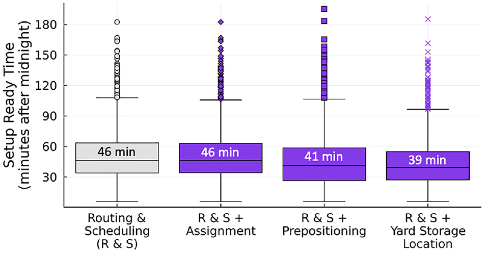
Overall setup ready times for RMM deployment strategies.

It was observed that the overall distributions did not change by a large magnitude when applying the three distance-minimizing strategies. The assignment strategy had a very similar distribution; the prepositioning and yard storage location strategies reduced the median RMM setup ready time by 5 and 7 min, respectively. The prepositioning model also had a slight effect on the variability of the setup ready time.

Across all of the results, setup ready times ranged from close to 0 min after midnight (for cases in which an RMM’s work zone was very close to its yard, with no revenue vehicles in its way) to over 180 min after midnight for the most extreme cases. These higher values reflect a variety of possible factors that affect the routing and scheduling model, with the most significant factors being the availability of tracks for RMMs based on revenue train movements (which can occur later in the night owing to special events, unplanned disruptions, or tracks being taken out of service for major projects) and longer travel distances—direct trips between two stations on the WMATA network may be as long as 49 mi.

However, it is important to note that each distance-minimizing strategy only applies to a subset of the RMMs owing to operational constraints (e.g., the additional workload for rail traffic controllers created by prepositioning RMMs, which is constrained in the solutions), which has a limiting effect on the overall efficacy of each strategy. Therefore, it is worth investigating each strategy further by breaking down RMM trips in the distribution by those whose trip origin changed relative to the baseline results because of one of the strategies and those whose trip origins did not change.

Figure 8 includes two boxplots for each of the three distance-minimizing strategies. The boxplots show the distributions of the difference in setup ready times between the baseline results and the results with a distance-minimizing strategy performed. A negative value in the difference in setup ready time means that the particular RMM trip was able to set up at its work zone earlier with the distance-minimizing strategy applied to all RMMs relative to the baseline. Each strategy includes a red boxplot showing the distribution of the difference in setup ready times for RMMs whose deployment plans are identical to the baseline routing and scheduling model without any distance-minimizing strategies applied (i.e., not reassigned, prepositioned, or receiving a new yard storage location), and a blue boxplot showing the distribution of the difference in setup ready times for RMMs that received a new deployment plan under the strategy.

Figure 8.

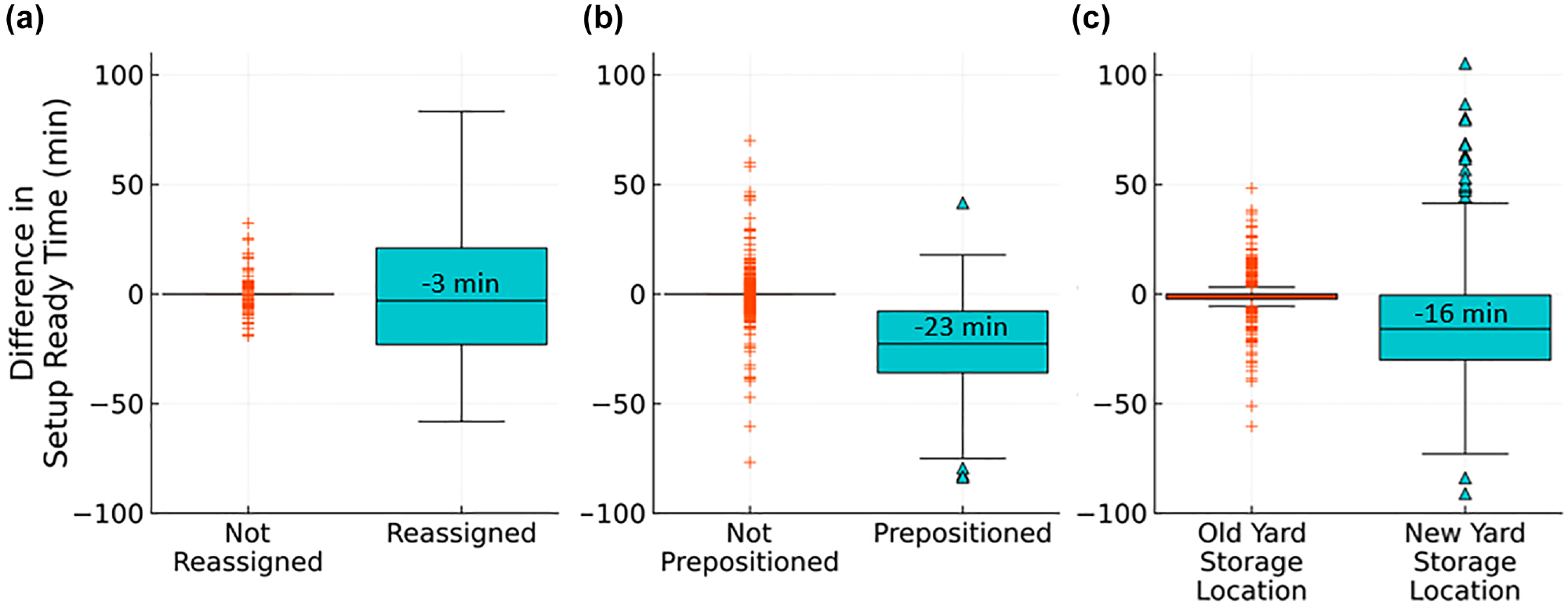
Impacts of deployment strategies on targeted and untargeted RMMs: (a) assignment, (b) prepositioning, and (c) yard storage location.Note: RMMs = roadway maintenance machines.

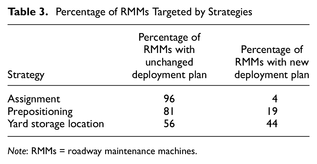
In addition, Table 3 shows the percentages of RMMs with unchanged and new deployment plans, respectively, out of the 1,225 total RMM trips included.

Table 3.

Percentage of RMMs Targeted by Strategies

Strategy	Percentage of RMMs with unchanged deployment plan	Percentage of RMMs with new deployment plan
Assignment	96	4
Prepositioning	81	19
Yard storage location	56	44

Note: RMMs = roadway maintenance machines.

Beginning with the assignment strategy shown in Figure 8a, it was apparent that the mostly unchanged overall setup ready time distribution relative to the baseline observed in Figure 7 could be attributed to 1. the low proportion of RMMs that were reassigned by the assignment strategy (4% of the total), and 2. the generally low difference in setup ready times experienced by the reassigned RMMs. Point 1 can be explained by the operational consideration that only in-service RMMs with identical consists are eligible for reassignment; even though certain classes of RMMs are interoperable, their consists are frequently tailored to a specific variety of work (e.g., a flatcar loaded with rail replacement materials), limiting the potential for reassignment. Point 2 can be explained by the RMMs already being assigned by jurisdictions that are geographical in nature, limiting the opportunities for reassignment.

The prepositioning strategy plots, shown in Figure 8b, show a greater improvement from this strategy relative to the baseline. Some 19% of RMMs were prepositioned, and the median prepositioned RMM was able to set up 23 min earlier than in the baseline scenario. It should be noted that although prepositioning had the highest potential benefits for affected RMMs of the three strategies, there were also major operational considerations that limited the applicability to only 19% of total RMMs. Firstly, it does not make sense to preposition an RMM whose work zone would prevent other RMMs from bypassing it by occupying both tracks (e.g., to perform maintenance on a structure shared by both tracks), as this means it will still have to wait for other (nonprepositioned) RMMs to pass by it before being “setup ready,” negating the benefits of having prepositioned closer to the work zone. Secondly, in a high-frequency urban rail network, prepositioning may result in an increase in rail traffic controller workload owing to the challenges of operating RMMs and revenue vehicles in mixed traffic. These results constrained the prepositioning movements to one RMM per operational jurisdiction (WMATA has four, meaning no more than four RMMs could be prepositioned on a given night).

Finally, the yard storage location strategy plots shown in Figure 8c indicate that 44% of RMMs received a new yard storage location and that the median RMM that received a new yard storage location had a setup ready time 16 min earlier than in the baseline scenario. Although the individual benefit from a new yard storage location was lower than that of prepositioning, the wider applicability of the yard storage location means that the overall benefit to the system is greater. The longer planning horizons associated with developing new long-term storage locations at yards means that the operational considerations of this strategy relative to the other strategies are not as limiting.

It should be noted that, for all three of the distance-minimizing strategies, the RMMs that did not receive reassignment, prepositioning, or a new yard storage location (i.e., those represented in the orange boxplots in Figure 8) usually did not see major changes. Although there are some outliers, the whiskers of the boxplots are at or near zero, indicating that most of the time, an RMM that is not able to take advantage of one of the distance-minimizing strategies usually will not be penalized.

Limitations

Observing the results in Figure 8, it was apparent that the distance-minimizing strategies can result in significant increases in the setup ready times for some individual RMM trips. For the yard storage location strategy, this outcome was unavoidable: given the capacity limitations of yards, some RMMs will have to be stored on the periphery of the network, and these RMMs are likely to incur longer travel distances and later setup ready times. However, the prepositioning strategy did not directly disadvantage individual RMMs from a distance-minimization perspective (as prepositioning is always optional). Therefore, the existence of prepositioning instances that resulted in an increase in the setup ready time relative to the baseline routing and scheduling strategy implies that the solutions were not optimal from a time-minimization perspective: in an optimal time-minimization solution, prepositioning would have not occurred and impacts on other RMMs would have been minimal. These problems arose because minimizing travel distance does not always result in minimizing the setup ready time.

Although travel distance is a major factor in determining how early RMMs will reach their destinations, there are other factors that are considered within the routing and scheduling strategy but not by the distance-minimizing strategies. These factors include the schedules of the last revenue trains, which determine when tracks become available for RMMs to move through the network; conflicts between RMMs; and detouring to avoid crossing other work zones (thereby preventing them from setting up earlier). For example, one of the outcomes of the yard storage location strategy was to store a large variety of RMMs at Brentwood Yard, the only yard in the WMATA network located close to the geographic center of the system. This maximized the number of trips that could originate from the center of the network, reducing instances where RMMs must travel to the center from yards on the periphery of the network. However, as can be seen in Figure 9, the magnitude and variability of RMM departure times from Brentwood Yard increased as a result of this practice. Although the delays incurred by additional RMMs exiting Brentwood Yard did not outweigh the overall benefits, it is possible that in other situations this kind of congestion would be detrimental to the overall system. Future research on the strategies could incorporate these distance-minimizing decisions more fully into the routing and scheduling model to consider the effects of conflicts and other elements of travel time.

Figure 9.

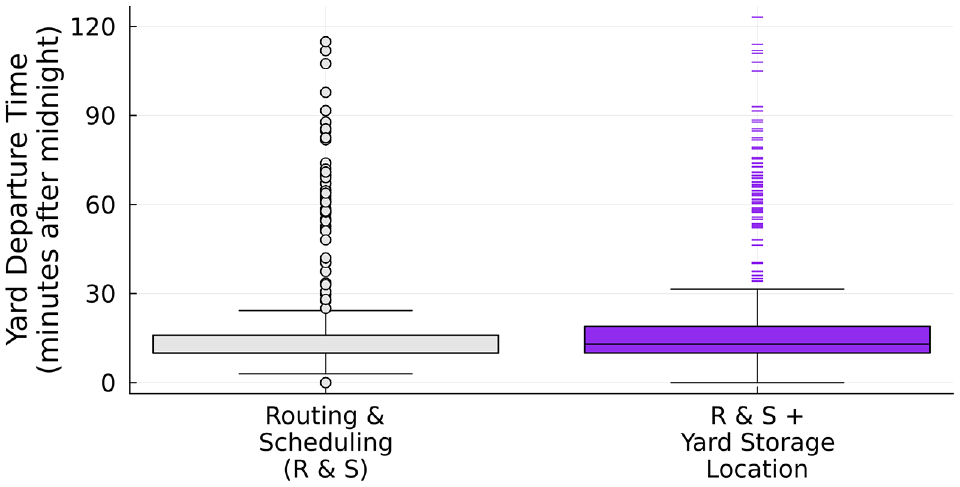
Yard departure times from Brentwood Yard.

Finally, although it was stated earlier that work events are often planned before and independently of RMM deployment planning in the urban rail context, the variability of the setup ready times shown in Figures 7 and 8 implies that the initial input conditions to the models (e.g., locations of work zones, revenue schedules) had a significant impact on the outcomes. It is likely that incorporating RMM deployment effectiveness into the planning of work events and the scheduling of last revenue trains and deadheading trains could increase the effectiveness of these strategies.

Conclusion

This paper demonstrates the potential of improving RMM deployment planning to increase the available time for maintenance activities on urban rail networks. Several strategies have been identified, encompassing both strategic planning (yard storage location) and tactical/operational planning horizons (assignment, prepositioning, and routing and scheduling). These strategies, which can be modeled as mixed-integer optimization problems, were evaluated using the real-life data and network of WMATA.

Three distance-minimizing strategies were evaluated, and the impacts on available time for maintenance activities were estimated by using the recommendations from these strategies as inputs to the routing and scheduling model. It was found that the prepositioning strategy had the largest reduction in deployment time on individual RMMs that could be prepositioned (median 23 min), whereas the yard storage location strategy could be applied to the greatest number of RMM trips (44%, with a median deployment time reduction of 16 min).

The value of the routing and scheduling model was also demonstrated as a tool to assess the timing of RMM deployment based on the distance-minimization strategies chosen, incorporating conflicts between RMMs, the availability of tracks to avoid disrupting revenue service, detouring to avoid passing through active work zones, and the use of crossovers. This analysis helps to refine the distance-minimization approach, and future research could pursue further integration between the various distance-minimization strategies and the time-minimization approach of the routing and scheduling model.

Footnotes

Acknowledgements

The authors would like to thank various staff and groups at the Washington Metropolitan Area Transit Authority for their input and collaboration. In addition, the authors would like to thank members of the MIT Transit Lab for overall feedback on the research direction and presentation.

Author Contributions

The authors confirm contribution to the paper as follows: study conception and design: J.T. Moody, H.N. Koutsopoulos; data collection: J.T. Moody, H.N. Koutsopoulos, M. Eichler, Y. Ulysse; analysis and interpretation of results: J.T. Moody, H.N. Koutsopoulos, M. Eichler, Y. Ulysse; draft manuscript preparation: J.T. Moody, H.N. Koutsopoulos. All authors reviewed the results and approved the final version of the manuscript.

Declaration of Conflicting Interests

The authors declared the following potential conflicts of interest with respect to the research, authorship, and/or publication of this article: J.T. Moody and H.N. Koutsopoulos received funding from the Washington Metropolitan Area Transit Authority (WMATA), the case study in this research. M. Eichler and Y. Ulysse are employees of WMATA.

Funding

The authors disclosed receipt of the following financial support for the research, authorship, and/or publication of this article: Funding for this research was provided by the Washington Metropolitan Area Transit Authority through their Academic Research Partnership with the MIT Transit Lab.

ORCID iDs

John Takuma Moody

Haris N. Koutsopoulos

Michael Eichler

Yann Ulysse

References

Lynch

Boston Track Map. 2023. https://www.vanshnookenraggen.com/_index/docs/Boston_MBTA_TrackMap.pdf.

SFMTA. Muni Metro Light Rail. 2023. https://www.sfmta.com/getting-around/muni/muni-metro-light-rail.

Cambron

J. R.

WMATA 129 Mile System Track Map. 2023. https://cambronj.blogspot.com/2020/12/wmata-129-mile-system-track-map.html.

Liao

Wang

Integrated Optimization of Bus Bridging Route Design and Bus Resource Allocation in Response to Metro Service Disruptions. Journal of Transportation Engineering, Part A: Systems, Vol. 148, No. 8, 2022.

Gkiotsalitis

Cats

Optimal Frequency Setting of Metro Services in the Age of COVID-19 Distancing Measures. Transportmetrica A: Transport Science, Vol. 18, 2022, pp. 807–827.

Lopez

Centeno

Integrated System to Maximize Efficiency in Transit Maintenance Departments. International Journal of Productivity and Performance Management, Vol. 55, 2006, pp. 638–654.

Dai

Ding

Qin

Multi-Component System Maintenance Optimization of Rail Transit Train Based on Opportunistic Correlations. Transportation Safety and Environment, Vol. 5, No. 4, 2023, p. tdad005.

Murakami

Turnquist

M. A.

Dynamic Model for Scheduling Maintenance of Transportation Facilities. Transportation Research Record: Journal of the Transportation Research Board, 1985. 1030: 8–14.

Lid’en

Kalinowski

Waterer

Resource Considerations for Integrated Planning of Railway Traffic and Maintenance Windows. Journal of Rail Transport Planning & Management, Vol. 8, 2018, pp. 1–15.

10.

Balakrishnan

Roth

Effectively Solving Production Gang Scheduling Problems for Railway Track Maintenance Projects. INFORMS Annual Meeting, 2009.

11.

Lynch

New York City Track Map. 2023. https://www.vanshnookenraggen.com/_index/docs/NYC_full_trackmap.pdf.

12.

Jarrier

Detailed Map of London Tube, Underground, Overground, DLR, Tramlink & National Rail. 2023. https://cartometro.com/metro-london/?r=cmf.

13.

Nguyen

H. T. M.

Chow

A. H. F.

Ying

C.-S.

Pareto Routing and Scheduling of Dynamic Urban Rail Transit Services With Multi-Objective Cross Entropy Method. Transportation Research Part E: Logistics and Transportation Review, Vol. 156, 2021, p. 102544.

14.

Yao

Zhu

Shi

Shang

Last Train Timetable Optimization Considering Detour Routing Strategy in an Urban Rail Transit Network. Measurement and Control, Vol. 52, 2019, pp. 1461–1479.

15.

Zhong

Zhang

Wang

Zhong

Wen

Peng

A Mixed Integer Linear Programming Model for Rolling Stock Deadhead Routing before the Operation Period in an Urban Rail Transit Line. Journal of Advanced Transportation, Vol. 2020, 2020, p. e3809734.

Strategies to Optimize the Deployment of Roadway Maintenance Machines for Overnight Maintenance in Urban Rail Systems

Abstract

Keywords

Literature Review

Problem Statement

Methodology

Yard Storage Location

Assignment

Prepositioning

Routing and Scheduling

Case Study

Results and Discussion

Limitations

Conclusion

Footnotes

Acknowledgements

Author Contributions

Declaration of Conflicting Interests

Funding

ORCID iDs

References