Sage Journals: Discover world-class research

Abstract

In this paper, we present a digital twin approach to the enhancement of traffic signal performance monitoring and congestion identification using automated traffic signal performance measure (ATSPM) systems. The objective of this effort is to use the high-fidelity microscopic simulation engine to generate simulated traffic signal events and connected vehicle data and allow the ATSPM systems to generate various traffic signal measures of effectiveness (MOEs) for a forensic traffic signal evaluation. Real-world ATSPM systems are driven by the traffic signal logs generated during operations. Therefore, they are primarily applied to traffic signal operations in the field. However, traffic signal design at present still follows the traditional method based on averaged delays, stops, and so forth, while more and more agencies have begun to evaluate the implemented traffic signal systems’ performance using the novel ATSPM MOEs. The proposed ATSPMs-in-the-loop simulation system fills this gap by using the ATSPM systems to evaluate the proposed traffic signal timings at the design stage. The benefits of this system include providing full-spectrum decision support for traffic signal management from design to operation and facilitating agencies to develop new insights on identifying traffic signal problems using the ATSPM MOEs. Another feature of the ATSPMs-in-the-loop simulation system is that it can use the emerging connected vehicle data set to generate new traffic signal MOEs. In the case study, we demonstrate how to use the proposed system to identify the potential issues of detector layouts and bottlenecks. Additional features of this ATSPM digital twin include allowing external components to interact with this platform via standard protocols in traffic control systems and connected vehicles to serve more purposes.

Keywords

operations hybrid simulation macroscopic traffic simulation mesoscopic traffic simulation microscopic traffic simulation traffic signal systems signal timing

In this paper, we present an exploration of applying the state-of-the-art automated traffic signal performance measure (ATSPM) to traffic signal timing design. The ATSPM system represents the latest development in arterial traffic signal management. By logging individual control events, such as detector actuation or phase transitions, the ATSPM system enables the development of novel traffic signal performance measures (SPMs) other than the traditional averaged ones. After more than a decade of collective efforts by agencies, companies, and academia, the concept of the ATSPM system has been commonly accepted by the community and many agencies have installed it or expressed an interest. While this trend is inspiring, some challenges have also surfaced. A common concern is that the current state of ATSPMs appears to generate a gap between traffic signal design and traffic signal operations. While the ATSPM system’s new measures of effectiveness (MOEs) are indeed helping agencies to identify, reduce, and even prevent congestion in operations, those novel MOEs are barely considered at the stage of traffic signal retiming. At present, we are still using traditional MOEs, such as delays or stops, to optimize traffic signal timings, which have been criticized for inferior efficiency under complex traffic signal operations containing multimodal or congestion data. As a result, it would be necessary to introduce the ATSPM concept into the full spectrum of traffic signal operations, from design to operations. Another issue is that the current ATSPM system is mostly based on the events of fixed-spot detectors but lacks the accommodation of probe-based traffic data. Meanwhile, many mobility data sources from smartphones or in-vehicle communication modules have come to the market recently and become accountable data sets for traffic signal operations. Therefore, it is necessary to enhance the ATSPM system to take advantage of all available data sets.

We developed a digital twin approach to fill the above gaps. Through customized communication modules, we built an “ATSPMs-in-the-loop” system to couple a microscopic simulation engine, PTV VISSIM ( 1 ), with two full-scale ATSPM systems: the open-source ATSPM system contributed by Utah Department of Transportation (UDOT) and the big-data-enhanced ATSPM module developed by Li et al. ( 2 ). Special programs were also built to parse the simulation outputs to ATSPM-compliant traffic signal events and vehicle waypoints and then feed them into the ATSPM systems. The objective of this effort is to adopt the same measures for both traffic signal design and traffic signal operations. In particular, when traffic conditions become complicated, such as multimodal and/or congestion conditions, the proposed approach can provide quantified evaluations of the proposed traffic signal timings. In contrast, the current practice can only provide a baseline traffic signal timing and then must be empirically adjusted to accommodate those complexities. The final deliverables of this effort will include publicly available software packages to couple traffic simulation and ATSPM systems and make them ready for implementation for both research ideas and regular practice. The objective of this effort is to introduce the concept of ATSPMs to a broader audience and facilitate interested users to evaluate and design complex traffic signal operations using the ATSPM digital twin. Such topics include but will not be limited to adaptive traffic control, trajectory-based traffic control, and multimodal, preemptions, or unconventional intersection design control. In other scenarios, the ATSPM digital twin can be used to determine a strategy for detector deployments at intersections. In practice, many existing intersections do not have sufficient detection resources for a fully functional ATSPM system. The ATSPM digital twin can be easily enhanced to estimate the system’s effectiveness under various detector configurations.

The rest of this paper is organized as a literature review on the emerging traffic big data, ATSPMs, and digital twinning, followed by a description of the ATSPMs-in-the-loop simulation framework. Then we describe how to pre-process the commercial connected vehicle (CV) data and how to generate the simulated CVs. Next, we described the simulation model development and calibration, following the recommendations, using the latest version of the traffic simulation toolbox ( 3 ) and traffic system simulation manual ( 4 ). Finally, we provide a demonstration using Cooper Street in Arlington, Texas, a freight corridor specified by the Texas Department of Transportation (TxDOT).

Literature Review

Emerging Traffic Big Data for Traffic Signal Systems

Travel speed data from Google Maps: Google is the largest map service provider in the world. The Google Maps platform provides more than 99% coverage of the world’s roads, has 1 billion active users per month, and collects the geolocation of millions of smartphone users. Thus, the sample available to Google that can be used to provide estimates of traffic conditions is significantly larger than that used by other services. Google products also leverage its in-house powerful algorithms for data fusion and artificial intelligence. Google makes real-time route travel time available for four modes: driving, public transit, walking, and biking. Google has recently changed its policy on its map application programming interfaces (APIs), allowing developers to use the real-time travel time information out of its map engine. This new policy opens avenues for applying Google travel time information to novel traffic applications. With such APIs, users can obtain real-time route travel time from the Google Maps server according to specified travel modes and specified routes. The returned route travel times can be integrated with new or existing congestion management systems. Since no hardware is required, it is possible to dynamically adjust the project scope and querying schedule. Google also provides travel times along user-defined corridors on request, which may be used to understand congestion patterns with quantified indicators, such as the arterial level of service. Unlike data from other providers (such as INRIX), corridor-level information is only available after users define such a corridor, which means that it is not possible to analyze a corridor for dates before the beginning of the study. The authors has built the Google travel time data feed into its ATSPM system.

CV data: The Internet-CV data, also referred to as geospatial-temporal data, is emerging in parallel to dedicated short-range communications vehicle-to-everything (DSRC-V2X)-based vehicle technology. The CV data is a type of “passively crowdsourced” data, containing significantly important information about the traffic flow. Most currently manufactured vehicles contain embedded high-end Global Positioning System (GPS) and cellular modules for location services (e.g., GMC’s “OnStar” and Toyota’s “SOS”). Even without a subscription, auto manufacturers regularly collect vehicle information for multiple purposes. Non-personal information is further redistributed (e.g., Wejo data [ 5 ]) for various kinds of analysis. With the rapid development of mobile and cloud computing as well as the proliferation of the Internet-of-Things (IoT), an increasing amount of such data is becoming readily available. In Texas, CV data represent 2%–6% of all moving vehicles ( 6 ). High-fidelity CV data offers potentially groundbreaking information, which, if harnessed, can solve some longstanding grand challenging problems. Compared with other commercial data or project-driven vehicle GPS trajectories, some features of CV vehicle data include unprecedented fidelity, precise lane-level positioning, satellite-grade timestamping, and exceptional penetration rates from one single data source (see the Data Reduction and Processing for Regions of Interest section, for example). These new features offer great potential for transportation mobility and management. Nonetheless, processing and interpreting this new data set are challenging because the data size is often of the order of terabytes. In general, Ahmad et al. ( 7 ) leveraged CV data to assess the operational aspects during an emergency evacuation prompted by a wildfire on short notice. The study aimed to highlight the benefits of the CV data set. The authors successfully demonstrated that such data could serve as an effective tool for accurately evaluating traffic delays and overall traffic operations during specific events and timeframes.

INRIX data: INRIX ( 8 ) provides probe-based speed levels at a very fine spatial and temporal resolution covering a significant portion of the roadway network, which includes both freeways and surface roads. The data is provided over segments of varying lengths and consists of average speeds/travel times every minute computed based on a sample of GPS points from participating vehicles. The data includes estimates of the reliability of the data based on the sample size, as well as estimates of typical traffic conditions in each segment. The spatial and temporal coverage of INRIX data, which is available as far back as 2015 in some areas, makes it a promising source to model congestion patterns while considering seasonal and daily variations, as well as spatial correlations. INRIX also makes congestion analysis tools available through the INRIX analytics platform, and the Center for Advanced Transportation Technology (CATT) laboratory has developed a suite of data analysis tools that may be leveraged for congestion management. These include products based on the trajectory information collected from participating vehicles, including origin–destination (O-D) matrices, selected-link analyses, and route analyses. Such products may support the development of comprehensive arterial traffic management strategies by allowing for macroscopic-level analyses of trip patterns and route choices. TxDOT has a contract with INRIX for state-wide probe travel times.

Streetlight data: Streetlight Data, Inc. ( 9 ), integrates multiple public and commercial data sources of location data, including GPS devices, location-based services, and micro-mobility services. Its data partners include INRIX, Siemens, and Forum Analytics. Streetlight provides an interface to retrieve and analyze historic trajectory data using different methods: users can place “gates” across roads and retrieve comprehensive data for trips passing through them or users can draw “zones” and analyze travel patterns between them, including trips originating at, ending at, or passing through such zones. The analysis platform also includes more advanced capabilities to diagnose complex transportation problems and support congestion management. Streetlight is used by Transport Canada, as well as departments of transportation (DOTs) in many states including Florida, Iowa, Maine, Minnesota, and Virginia. Streetlight data were instrumental in resolving congestion issues in Napa Valley, California, where the data provided key information about internal and external trips and travel patterns that were not available from other sources. Similarly, in the downtown districts of Lafayette, California, Streetlight was used to deduce why traffic congestion occurred.

Waze traffic alerts and travel time data: Waze, Inc. ( 10 ), is a Google company and so Google Map data and Waze data are similar in delivering travel information based on millions of Android smartphone users. Unlike Google Maps data, Waze data is available to public agencies for free in exchange for the incidents reported by public agencies. To retrieve Waze Travel time data, participating agencies first need to apply for an account on the Waze TrafficViewer platform. Under approved accounts, the agencies can define the routes of their interests and then download the route travel times using the provided URL and unique ID.

Automated Traffic Signal Performance Measures

Most intersections controlled by mainstream traffic signal controllers today are equipped with high-fidelity data collection capabilities to feed the needed data for the ATSPM system. According to the National Electrical Manufacturers Association (NEMA) requirement ( 11 ), the resolution of traffic signal events is 10 Hz (1/10 s). The ATSPM performance reports contain information on vehicle phase changes, pedestrian walk signals, vehicle passing, and detector activations ( 12 ). Deployment of the ATSPM system requires updating the traffic signal controller with high-resolution data logging capability. Many agencies have adopted the ATSPM system at various scales. To name a few, the New Jersey Department of Transportation (NJDOT) employed SPMs in conjunction with existing traffic data to assess the need for additional equipment to improve their SPM system ( 13 ). Furthermore, its system performs well in monitoring the dynamics at signalized intersections and offers additional advantages over project-driven methods. As the most extensive deployment across the country, UDOT used the data derived from its ATSPM system to cross-check traffic counts data ( 14 ). In its study, various regression models were developed based on ATSPM data to assess the performance variations among different types of detectors, demonstrating a new potential of the ATSPM system. The Michigan Department of Transportation (MDOT) adopted the ATSPM system to conduct a cost–benefit analysis ( 15 ). It was found that each intersection yielded an approximate benefit of US$159,116 per year, resulting in a favorable cost-to-benefit ratio of 1:25. In another study, Mathew et al. ( 16 ) utilized precise trajectory-based data, not limited to traffic counts, to establish performance metrics for a bus rapid transit (BRT) system in Indianapolis, Indiana. Their research offers valuable methodologies enabling transportation experts to pinpoint scheduling modifications and substantiate investment choices. Furthermore, Jackson et al.’s ( 17 ) research emphasized transit-specific performance metrics, combining data from the bus system, specifically transit signal priority, with traditional ATSPMs. Tahsin Emtenan and Day ( 18 ) investigated the correlation between probe vehicle data and ATSPMs. Their study revealed a strong correlation between the two data sets, allowing the integration of CV data with software-in-the-loop (SILS) to generate high-resolution ATSPM data for further evaluation. In a separate study, Day et al. ( 19 ) proposed a method for evaluating corridor performance at the system level using high-resolution data. Several other studies, such as those involving cost–benefit analysis, optimization of traffic signal offsets, and the impact of detector configuration, have utilized detailed traffic signal event data for their analyses ( 20 – 22 ). Apart from this, Dumitru ( 23 ) conducted a unique analysis, exploring the impact of school bus traffic on a coordinated network of traffic signals. Notably, his study focused on a vehicle type that has received limited attention in urban areas. To enhance the credibility of his findings, Dumitru integrated a third-party ATSPM solution, providing a validated perspective on the identified problem. This exemplifies the significant advantages of ATSPM deployment by providing valuable insights on traffic conditions.

Simulation Model Calibration

It is necessary to consider all potential scenarios that may arise and complicate matters. A simulation study is preferred before the deployment. Microscopic simulation is widely adopted in traffic signal operations ( 24 ). These simulations have garnered substantial interest from users to estimate and predict certain measures that are challenging to collect in the real world. To ensure the simulation reflects reality, simulation models must be calibrated by adjusting the input parameters to minimize the difference between the simulation output and the observations from the real world. Some research studies employ the fundamentals of traffic flow theory, focusing on elements such as speed and flow, to calibrate simulation models. For instance, So et al. ( 25 ) conducted the calibration of extensive microscopic traffic simulation models, covering six arterials with 160 signalized intersections. Their calibration criteria encompassed volume, speed, and travel time, with an additional sensitivity analysis. In a separate study, Stevanovic et al. ( 26 ) utilized field data on signal timing optimization, incorporating factors such as speed limits, 15-min turning-movement counts, and queue lengths at selected intersections to calibrate the VISSIM simulation model. They validated their outputs using GPS floating vehicle data. In contrast, Aghabayk et al. ( 27 ) prioritized driving behavior as a crucial component for calibrating microscopic simulation models. Their approach was based on an optimization algorithm through the VISSIM COM interface. The optimization was performed with particle swarm optimization in conjunction with parallel/multi-threading techniques, ensuring an automated calibration process was completed within a significantly reduced timeframe. Yu et al. ( 28 ) introduced a calibration approach for a microscopic simulation model applied to the Beijing BTR system based on the GPS data of probe vehicles. They employed the sum of squared error ( 29 ) as the MOE for calibration and advocated incorporating multiple MOEs, including queue lengths and delays, to further enhance the accuracy of the calibrated model. Sun et al. ( 30 ) conducted a comparative analysis to assess the performance of various simulation models. Specifically, they compared VISSIM and CORSIM in the context of an urban street network. The study also included a sensitivity analysis based on different MOEs, such as average control delay, average queuing, and traffic volume. The findings highlighted the importance of calibrating and selecting the appropriate simulation models according to the intersection type and level of saturation for each simulated scenario. Ge and Menendez ( 31 ) conducted a thorough sensitivity analysis ( 32 ), followed by a study on the initial screening of parameters. Because of the impracticality of calibrating every parameter in the model, calibration is focused on specific parameters, while a comprehensive sensitivity analysis is performed to observe the model’s response to variations in input. Hellinga ( 33 ) presented a methodological framework and outlined the necessary criteria according to the objectives. They provided a seven-step approach that includes (I) defining the study purposes and goals, (II) determining the needed data, (III) choosing appropriate MOEs ( 34 ), (IV) establishing evaluation criteria; (V) initial calibration, (VI) driver routing behavior modeling; and (VII) validation of the outputs. Traditionally, much of the evaluation relied on travel demand characteristics, while with the progress of technologies, data extraction and trimming have become integral components of the calibration process in contemporary applications. Maheshwary et al. ( 35 ) introduced a four-step methodology for calibrating micro-simulation software to accommodate heterogeneous traffic environments. In their approach, they identified the sensitivity analysis for travel time as a MOE using the Latin hypercube design ( 24 ). They further created the analysis of variance (ANOVA) and linear regression models for each specific vehicle classification to determine the influential factors on travel time. The findings suggested applying distinct sets of optimal driving behavior parameters for different vehicle classes. Bartin et al. ( 36 ) conducted a case study to demonstrate the calibration and validation process for large-scale traffic simulation networks. They achieved the goal by utilizing various data sources, such as throughput volume, travel time, and queue length comparisons, alongside generating an O-D demand matrix. In a more recent study, Oh et al. ( 34 ) introduced a stochastic approximation framework to address the demand estimation in a multimodal microscopic network simulation, employing sensor data. Notably, this approach considered the travel demand as a discrete variable, departing from the traditional continuous variable representation. The researchers utilized a sophisticated version of the simultaneous perturbation stochastic approximation (SPSA) model to minimize the least square objective, which quantified the distance between simulated and observed measurements. This optimization process facilitated the replication of point-to-point and stop-to-stop travel time distributions.

Automated Traffic Signal Performance Measures-in-the-Loop Simulation Framework

Figures 1 and 2 demonstrate the system framework and workflow of the ATSPMs-in-the-loop simulation system. In Figure 1, the traffic simulation engine, VISSIM, is set to output all raw simulation records including the vehicle trajectories, pedestrian trajectories, and traffic signal events (phase transition and detector actuation). While the native form of the simulation output contains most of the information for ATSPMs, it must be parsed to be ATSPM-compliant so that the real-world ATSPM system(s) can recognize and proceed with visualization and quantification. The traffic signal logs in the simulation output are parsed and archived in the database (SQL server) of the open-source ATSPM system contributed by UDOT and the simulated vehicle trajectories are parsed into the database of the big-data-enhanced ATSPM module, referred to as UTA-In-Motion or UTAIM. Another parsing program was developed to transfer traffic signal events data from UDOT’s ATSPM database into UTAIM’s database. Finally, users can view two sets of simulated ATSPM MOEs under the current and/or proposed traffic signal timings from the web interfaces. Note that the entire system architecture is the same as the deployment in the real world except that the traffic signal records will be directly extracted from the traffic signal controllers in the field and the CV data will be retrieved from the data distributor. Therefore, the ATSPMs-in-the-loop simulation framework is a digital twin of the real-world system.

Figure 1.

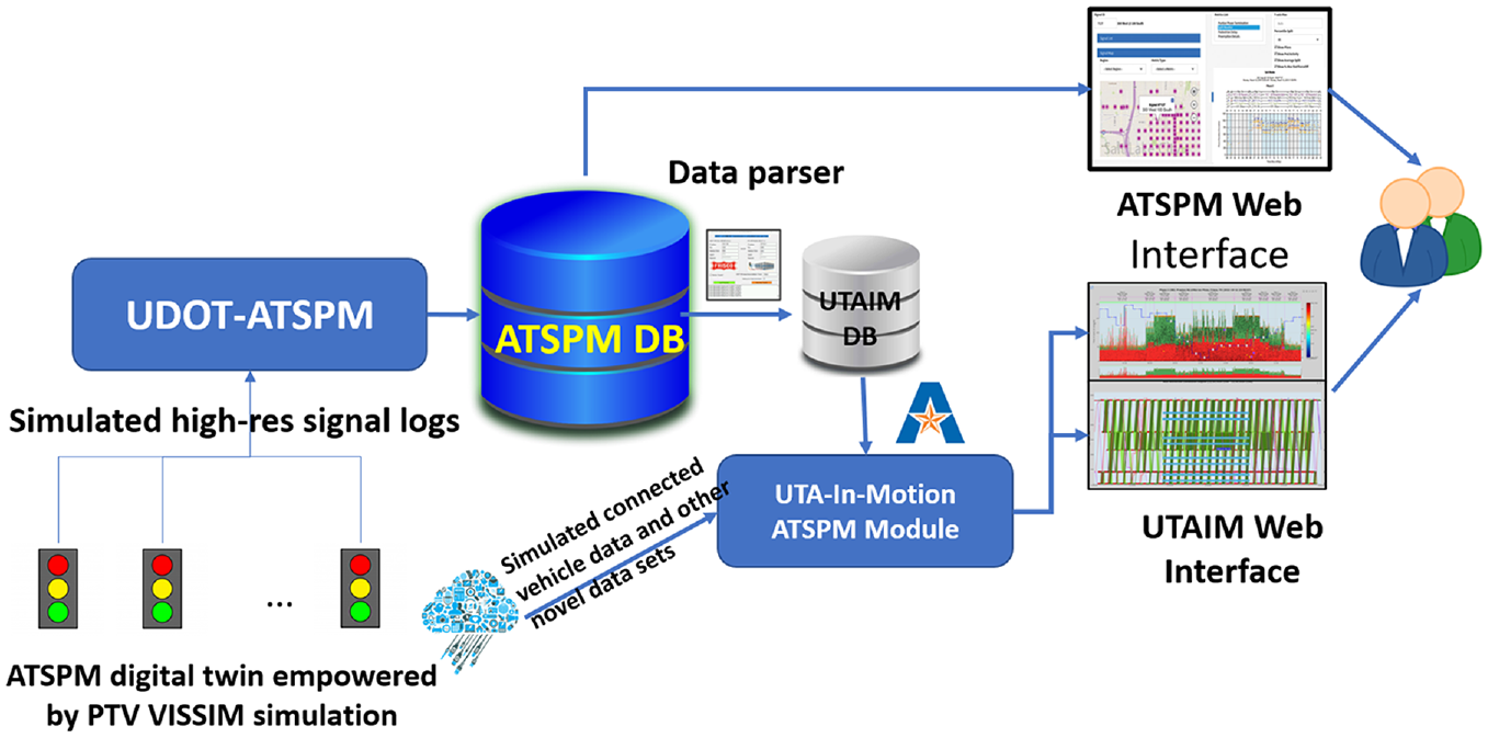
The system architecture of automated traffic signal performance measures (ATSPMs)-in-the-loop simulation.

Figure 2.

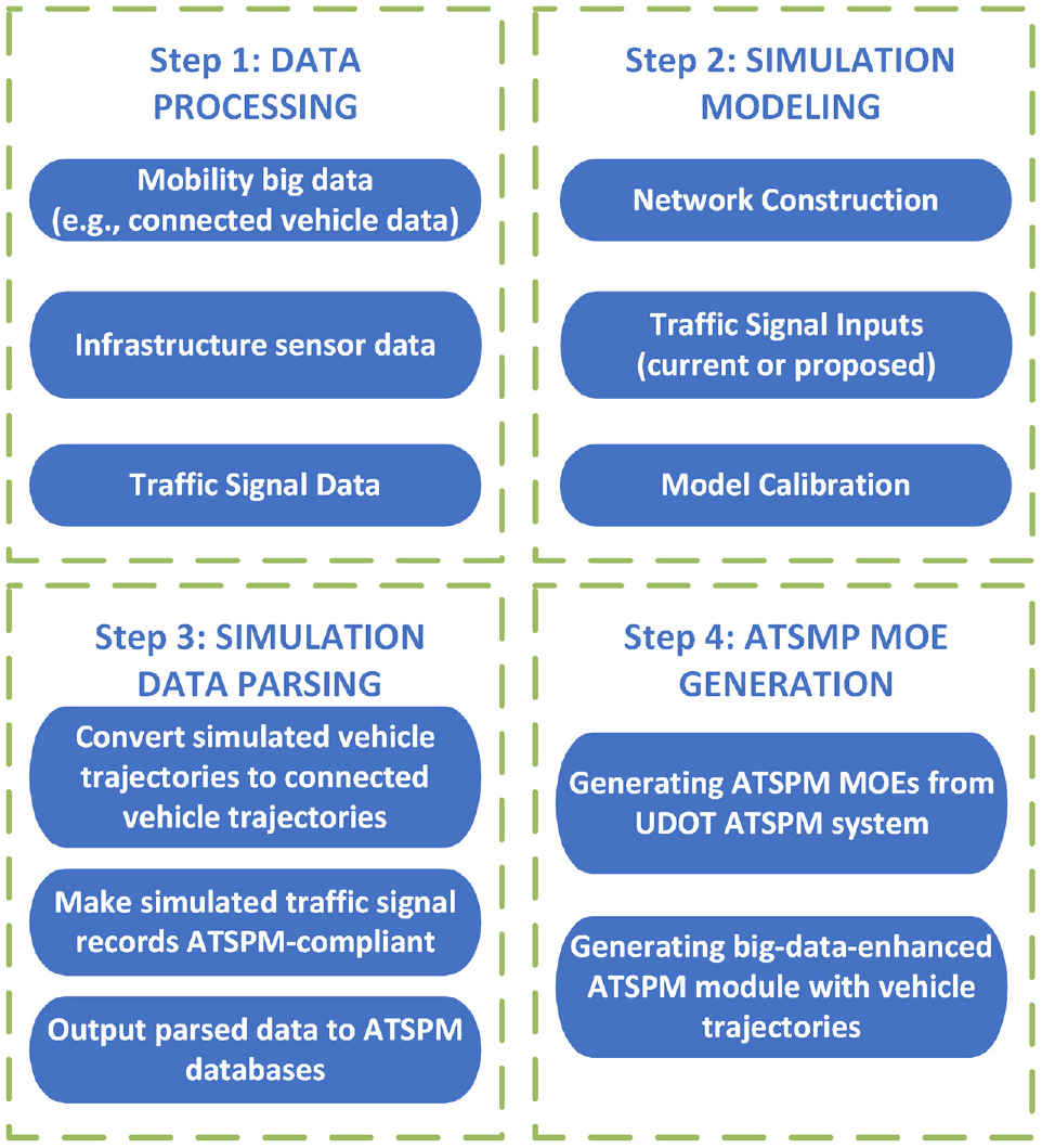
Workflow of data processing in the automated traffic signal performance measures (ATSPMs)-in-the-loop simulation.

Figure 2 shows the workflow of data processing. The first step is to prepare the necessary data for simulation modeling, including the infrastructure sensor data for traffic turning-movement counts, mobility big data for prevailing travel speed, and traffic signal data for baseline scenario construction. Based on these data, the simulation model will be constructed reflecting the road network geometry and traffic signal operations. It is also an important effort to calibrate the baseline model, including the traffic balance, travel time validation, turning-movement count validation, and so forth. Step 3 occurs after a simulation run is finished. The simulation output must be parsed to become ATSPM-compliant formats so the connected ATSPM systems can recognize it. The last step is to let the ATSPM systems generate and visualize the traffic signal performance based on the simulation results. This step is similar to operations in the real world except that it is for the proposed traffic signal timing during the stage of traffic signal design.

Connected Vehicle Data Processing

While the traffic signal timing data and traffic turning-movement counts can be obtained in a well-structured form at present, the emerging CV data have special challenges to be processed. The CV data offers new capabilities for improving the simulation model calibration.

Data Reduction and Processing for Regions of Interest

The CV data are often deliverable in large bulk to cover a region. Given the high granularity (vehicle trajectories with 1–3 s of intervals), the data size is often beyond the capability of regular data reduction techniques. For instance, the CV data size covering the Dallas-Fort-Worth metroplex is about 1.3 terabytes of compressed text files. Therefore, it is necessary to reduce the data to a manageable level. The data reduction requires generating a series of polygons to cover the regions of interest (ROIs). The ROIs are designed using any geographic information system (GIS) software in the Keyhole Markup Language (KML) format and an efficient data reduction approach, described by Khadka et al. ( 37 ), was employed to screen the regional CV data set and only keep those data within the ROIs. In this study, the ROIs around individual intersections are squares covering 250 ft back from the stop line of each approach and the ROIs along the segment of corridors are the polygons roughly along the right of way (ROW).

Map-matching: After the CV data set is reduced to the ROIs, the reduced data set must be further processed to screen out those irrelevant vehicle waypoints within the ROIs. As shown in Figure 3, the raw CV data sets do not only cover the roadways but also cover adjacent facilities accessible to vehicles, such as parking lots. Unless the CV data set is further screened, the irrelevant CV data set will significantly affect the following calibrations. The adopted technique here is map-matching. As shown in Figure 4, each vehicle’s waypoint will be compared with the road network at intersections to check if the vehicle was moving on the roadway or adjacent facilities according to its distance to the closest roadway. For more details of the map-matching techniques, readers are directed to Khadka et al. ( 6 ).

Figure 3.

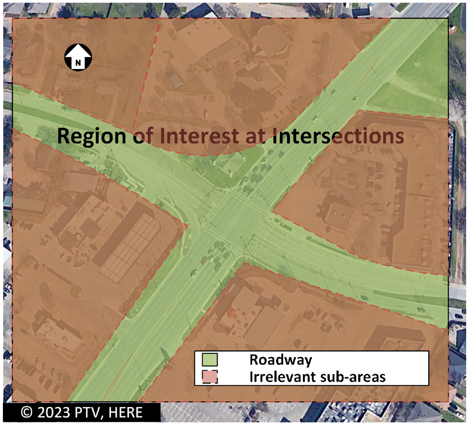
Demonstration of the region of interest at intersections and the reduced region on highways.

Figure 4.

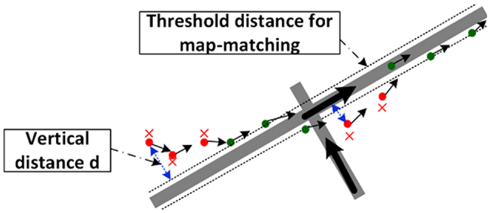
Map-matching for connected vehicle data processing.

Microscopic Simulation Modeling

In this section, we present the procedure of microscopic simulation modeling and calibration.

Network Construction

Network construction involves the development of a network layout for the target. The process varies depending on the simulation software used, with some focusing on volumes and turning movements, while others delve into more microscopic elements such as links and connectors. It is critical to ensure that all the model links and connectors are appropriately connected as intended. Any network discontinuity will adversely affect the entire network because the travel demand is formed with the continuous vehicle maneuvers until they leave the network. Another important element in the network construction is the yielding rules within conflict zones. Conflict zones refer to the locations where there are no traffic control devices, but vehicles have conflicts. As such, vehicles must follow certain rules to determine safe crossing, such as permissive right turn, permissive left turn, and so forth. The conflict zones should be designed based on the ROW rules governing vehicle maneuvers.

Vehicle inputs refer to travel demands. Depending on the simulation engine, the vehicle inputs can either refer to link flows or path flows. In VISSIM, the path flows are adopted by combining the vehicle inputs (from the network edges) and the defined vehicle routes. Most traffic counts are link-based at intersections in practice and the path flows can only be inferred through the probe data (e.g., CV data). A common problem with a vehicle turning counts is that they are not collected across intersections at the same time. Therefore, the outbound traffic from the upstream intersection may not be the same as the inbound traffic at the downstream intersection. To address this issue, multiple dummy inbound/outbound links must be added to allow excessive upstream vehicles to leave the network or supplement new vehicles to ensure the downstream travel demand is balanced. Figure 5 illustrates this concept.

Figure 5.

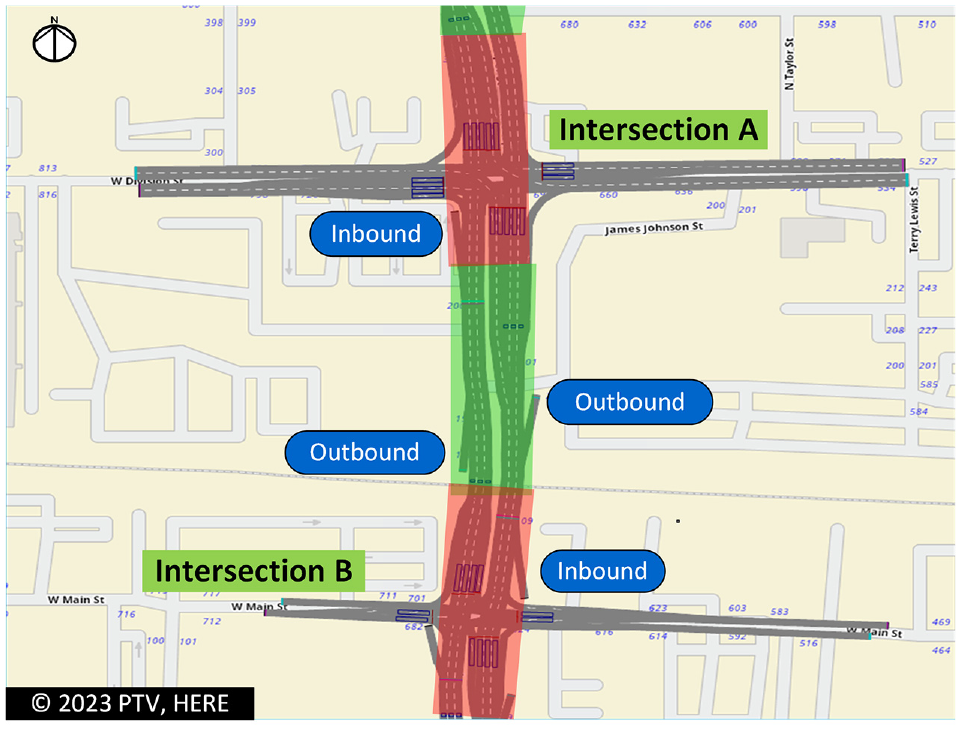
Flow balance through virtual vehicle inputs and exits between intersections.

Traffic signal timings: These can be downloaded from most traffic signal controllers nowadays. For instance, the local agency helped to download the entire database of each traffic signal controller (Siemens SEPAC) along the target corridor. Meanwhile, the local agency also provides the detector layouts at those intersections of interest. The time-of-day traffic control pattern and plan corresponding to the available vehicle turning-movement counts (e.g., peak hours during workdays) were pinpointed and summarized for the simulation model. Meanwhile, the detector layout, including the positions and channels, is also designed the same as the detector deployment in the field. To balance fidelity and simplicity, we chose the default signal control emulator in VISSIM, that is, the ring-barrier-control (RBC) module, to model the baseline signal timings. Figure 6 illustrates how the traffic signal components were designed in simulation according to the agency-offered detector layouts. The baseline simulation model replicates real-world traffic signal operations to the maximal capability of the RBC controllers.

Figure 6.

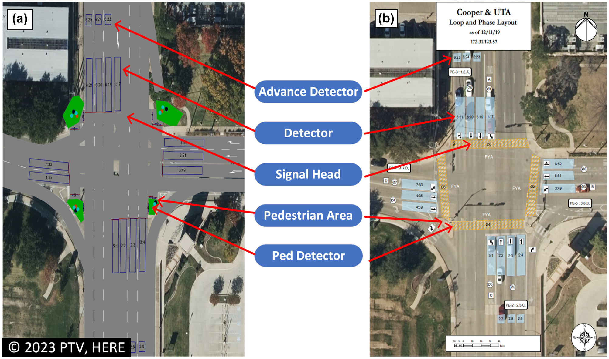
Traffic signal system comparison between the simulation (a) and the real world (b).

Simulation Calibration

Simulation calibration is critical to establish consistency between the baseline simulation model and the current traffic conditions. There are two categories of simulation calibration: countable measures and behavioral measures. The countable measures include turning-movement counts, queue lengths, and arterial travel times, while the behavioral measures include drivers’ desired speeds, driving aggressiveness, lane-changing collaborations, and so forth. While achieving consistency of countable measures is relatively easy in simulation by adjusting the simulation model’s vehicle inputs, routing decisions, and minimal safe headways in the simulation, most driving behaviors are not observable until the recent appearance of CV data. The measures to calibrate traffic simulation models include fine-tuning flows, routing decisions, speed distribution, and acceleration and deceleration functions. By optimizing these key components, the traffic simulation model can mostly comply with real-world traffic scenarios. The calibration parameters for these adjustments differ across various simulation models. The selected simulation engine for this study, VISSIM, offers plenty of flexibility for behavioral calibration. Its core car-following model is the Wiedemann car-following model, which covers comprehensive driving decisions ( 38 , 39 ). In contrast, other simulation software such as SUMO leans more toward route-based calibration using flow measurements ( 40 ). Flow calibration is inherently linked to volume calibration, as discussed in the earlier section on network construction. In addition to calibration with traditional turning counts and travel time, we also designed new methods for behavioral calibration with the CV data.

Countable Measure Calibration

Traffic counts calibration: Florida DOT published a traffic analysis handbook that covers the common techniques for traffic simulation calibration of countable measures ( 41 ). Table 1 outlines some of the calibration parameters. We also adopted similar methods to calibrate the countable measures.

Table 1.

Measures of Effectiveness (MOEs) for Calibrating a Model

Calibration measures	Tools	Calibration goal
Traffic volume	Node analysis	• Within 100 vph for volume less than 700 vph • Within 15 vph for volume between 700 and 2700 vph • Within 400 vph for volume greater than 2700 vph • Sum of link volumes to have GEH statistic value of 5 or lower
Travel time	Travel time measurement	• For travel time lower than 7 min, calibrated time should be in a range of ±1 min compared to actual travel time
Travel time	Travel time measurement	• For travel time higher than 7 min, calibrated time should be around 15% compared to actual travel time.
Speed	Data collection point	• Simulated average speed to be within ±10 mph of actual measured speed
Queue length	Queue counter	• Simulated and field-measured queue length should be within 20%
Intersection delay	Node analysis	• Simulated and field-measured link delay should be within 15% for more than 85% of cases
Visualization	Visual inspection	• Check for bottlenecks and unusual turns

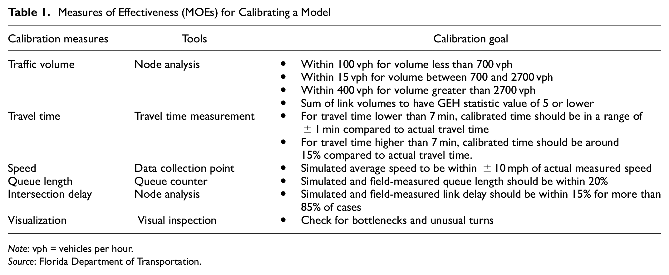
Note: vph = vehicles per hour.

Source: Florida Department of Transportation.

A common method for traffic simulation counts calibration model is the GEH statistic method, as shown in Equation 1. It is a formula used in traffic engineering to compare two traffic data sets. For traffic analysis, a GEH value of less than 5.0 is considered a good match between the modeled and observed hourly volumes ( 41 ):

GEH = \sqrt{2 \times \frac{{(M - C)}^{2}}{(M + C)}}

(1)

where M is the simulated volume and C is the actual counted volume.

There are also some additional procedures for calibrating a simulation model guideline that is provided by the Federal Highway Administration (FHWA) traffic simulation toolbox ( 3 ). The FHWA guidelines outline three specific steps for calibration:

identify representative days;

prepare variation envelopes;

calibrate the model with acceptable criteria.

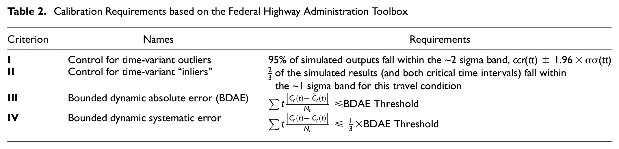
Representative time and date for baseline traffic conditions: In its latest version of the traffic simulation toolbox ( 3 ), FHWA provides instructions on how to identify representative days by analyzing time-dependent data related to important performance metrics. This analysis requires creating a 15-min profile as a critical measure to determine the representative day ( 4 ). Calibrating the model to meet the desired criteria involves modifying the parameters of the simulation models and evaluating the validation results against those criteria. This process requires multiple iterations and a considerable amount of time to achieve full calibration. Therefore, it is important to break down the calibration process into a set of logical and sequential steps, forming a strategic approach to calibration: parameters that the analyst is certain about and does not wish to adjust (e.g., incident location and number of lanes closed) and parameters that the analyst is less certain about and is willing to adjust (e.g., mean vehicle headway under low visibility conditions). The calibration of the model based on FHWA guidelines involves four distinct criteria. These criteria are outlined as follows.

Based on Table 2 for criteria III and IV, the bounded dynamic absolute error (BDAE) threshold is calculated as follows:

Table 2.

Calibration Requirements based on the Federal Highway Administration Toolbox

Criterion	Names	Requirements
I	Control for time-variant outliers	95% of simulated outputs fall within the ~2 sigma band, ccr(tt) ± 1.96 × σσ(tt)
II	Control for time-variant “inliers”	$\frac{2}{3}$ of the simulated results (and both critical time intervals) fall within the ~1 sigma band for this travel condition
III	Bounded dynamic absolute error (BDAE)	$\sum t \frac{\| C_{r} (t) - {\tilde{C}}_{r} (t) \|}{N_{t}} \leq BDAE Threshold$
IV	Bounded dynamic systematic error	$\sum t \frac{\| C_{r} (t) - {\tilde{C}}_{r} (t) \|}{N_{t}} \leq \frac{1}{3} \times BDAE Threshold$

BDAE Threshold = \frac{\sum i \neq r \sum t \frac{| C_{r} (t) - C_{i} (t) |}{N_{t}}}{N_{cluster} - 1}

(2)

where $C_{r} (t)$ is the observed value of a representative day during time interval t, $C_{i} (t)$ is the observed value of a non-representative day within the cluster during time interval t, ${\tilde{C}}_{r} (t)$ is the simulated performance measure during time interval t, $N_{t}$ is the number of time intervals, and $N_{cluster}$ is the number of days in the cluster representing this travel condition.

If all of the above conditions are satisfied, the model can be considered the final calibrated model. However, if any of these conditions are not met, it is necessary to adjust the parameters discussed in the calibration section and reevaluate all of these conditions from the beginning.

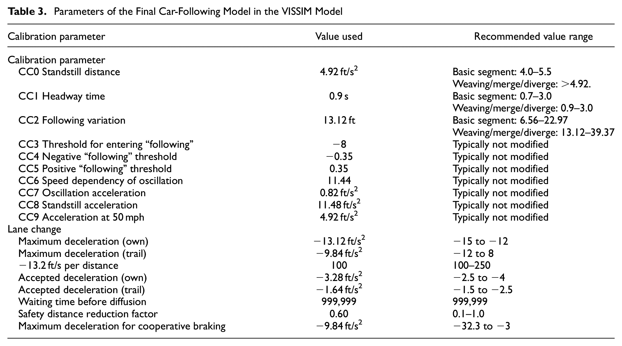
Capacity calibration by adjusting the car-following model: VISSIM adopted Wiedemann’s ( 38 ) car-following model, which includes various parameters such as standstill safety distance and additive and multiplicative components of the safety distance to determine the appropriate following behavior. Wiedemann 99 has 10 parameters that range from CC0 to CC9. All parameters refer to different aspects of driving behavior, such as acceleration, speed, time headway, and safety distance. Although there is literature on how to calibrate those parameters for model calibration in optimal ways, they are mostly not trackable. As such, the capability calibration was empirically performed by comparing the observed arterial travel time (observed from the CV data) and simulated arterial travel time, after the vehicle turning counts were calibrated. Table 3 shows the final car-following model in VISSIM, utilizing the recommended calibration parameter values sourced from the Traffic Engineering, Operations & Safety Manual issued by the Wisconsin DOT ( 42 ).

Table 3.

Parameters of the Final Car-Following Model in the VISSIM Model

Calibration parameter	Value used	Recommended value range
Calibration parameter
CC0 Standstill distance	4.92 ft/s²	Basic segment: 4.0–5.5 Weaving/merge/diverge: >4.92.
CC1 Headway time	0.9 s	Basic segment: 0.7–3.0 Weaving/merge/diverge: 0.9–3.0
CC2 Following variation	13.12 ft	Basic segment: 6.56–22.97 Weaving/merge/diverge: 13.12–39.37
CC3 Threshold for entering “following”	−8	Typically not modified
CC4 Negative “following” threshold	−0.35	Typically not modified
CC5 Positive “following” threshold	0.35	Typically not modified
CC6 Speed dependency of oscillation	11.44	Typically not modified
CC7 Oscillation acceleration	0.82 ft/s²	Typically not modified
CC8 Standstill acceleration	11.48 ft/s²	Typically not modified
CC9 Acceleration at 50 mph	4.92 ft/s²	Typically not modified
Lane change
Maximum deceleration (own)	−13.12 ft/s²	−15 to −12
Maximum deceleration (trail)	−9.84 ft/s²	−12 to 8
−13.2 ft/s per distance	100	100–250
Accepted deceleration (own)	−3.28 ft/s²	−2.5 to −4
Accepted deceleration (trail)	−1.64 ft/s²	−1.5 to −2.5
Waiting time before diffusion	999,999	999,999
Safety distance reduction factor	0.60	0.1–1.0
Maximum deceleration for cooperative braking	−9.84 ft/s²	−32.3 to −3

Behavioral Measure Calibration

We roughly define two driving conditions along arterials: stable driving where drivers have left the upstream intersection, reached their desired speed, and are stable for a while (the green zone in Figure 5); unstable driving while drivers are approaching or leaving an intersection where they will frequently accelerate or decelerate at their desired acceleration/deceleration rate (the red zone in Figure 5). The pre-processed CV data set is further divided into two groups according to the behavioral zone.

Speed distribution is summarized using the CV data during stable driving. It is a fundamental input in VISSIM for simulated vehicles reflecting vehicles’ free-flow speeds, which is critical to determine the offsets of coordinated traffic signal operations. The speed distribution is the statistical representation of the speed of simulated vehicles that are moving along a given roadway ( 43 ). Using the corresponding trajectories of CVs, one can determine the speed distribution during stable driving. Each vehicle’s instantaneous speed was compiled into a distribution, as illustrated in Figure 7.

Figure 7.

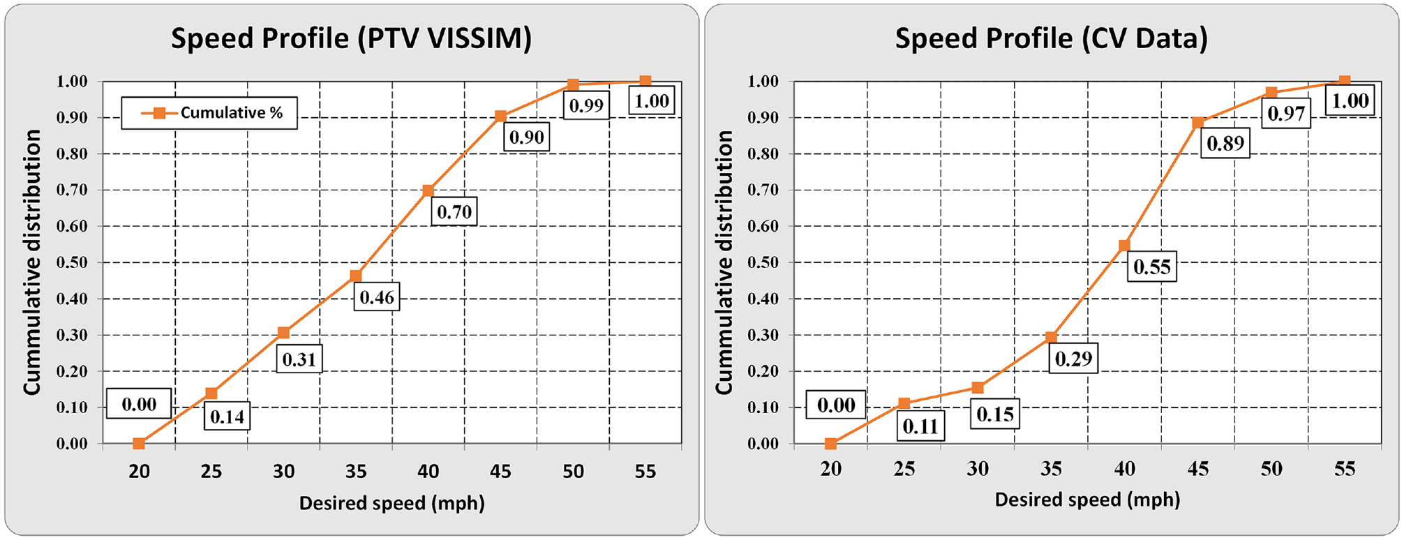
Speed distribution from simulation software and connected vehicle (CV) data.

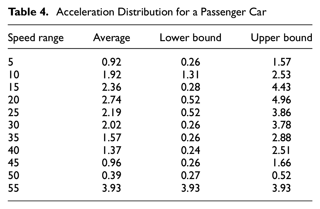
The desired acceleration/deacceleration distribution is critical to simulate driving behaviors adjacent to intersections. Jie et al. ( 44 ) emphasized that the acceleration and deceleration functions play a crucial role in influencing the saturation flow, acceleration, speed, and travel time. The acceleration and deceleration functions are represented in VISSIM by a curve revealing the acceleration/deceleration (in ft/s²) against the speed (in mph) on the Y and X-axes. The minimum and maximum acceleration can be estimated from the compiled CV data set and so are the average acceleration/deceleration rates against various speeds. In this study, the 25th percentile is used for the minimum acceleration/deceleration, and the 95th percentile is used for the maximum acceleration/deceleration. The acceleration distribution for a passenger car was derived from CV data and is presented in Table 4. Graphs of the acceleration functions are illustrated in Figure 8.

Table 4.

Acceleration Distribution for a Passenger Car

Speed range	Average	Lower bound	Upper bound
5	0.92	0.26	1.57
10	1.92	1.31	2.53
15	2.36	0.28	4.43
20	2.74	0.52	4.96
25	2.19	0.52	3.86
30	2.02	0.26	3.78
35	1.57	0.26	2.88
40	1.37	0.24	2.51
45	0.96	0.26	1.66
50	0.39	0.27	0.52
55	3.93	3.93	3.93

Figure 8.

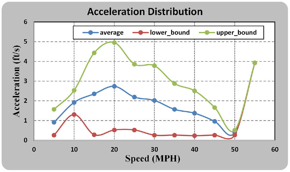
Acceleration function against driving speed according to the connected vehicle data.

Case Study: Bottleneck Identification using Automated Traffic Signal Performance Measures along Cooper Street in Arlington, Texas

The purpose of this case study is twofold:

examine if the developed ATSPMs-in-the-loop simulation system will work as intended;

develop new insights on how to identify traffic signal bottlenecks from the ATSPM MOEs as opposed to the known ground truth traffic (i.e., microscopic simulation animation).

The target arterial is Cooper Street in Arlington, Texas. It starts from Division Road and ends at the I-20 interchange, covering about 5 mi with 16 intersections. There are a few major–major intersections, and the speed limits also change in the middle of this arterial. As a result, the driving behaviors vary along the arterial and so we divided the arterial into three zones. The boundaries of the zones were set at major–major intersections and where the speed limit changes, as shown in Figure 9. The Cooper Street corridor was modeled in VISSIM with its RBC signal emulators. The modeling and calibrating processes followed the above methods. To avoid initial and end bias, the first and last 15 min of the volume data were duplicated for simulation warming up and cooling down. The overall simulation time was set for 2 h and 30 min but the actual data collecting time was just 2 h, excluding the initial and final 15 min. Aggregated simulation output was recorded every 5 min or every 300 s, and individual records of vehicles, pedestrians, and traffic signal operations were archived separately. The model evaluation was configured to begin data recording after 15 min and end 15 min before the end of the simulation.

Figure 9.

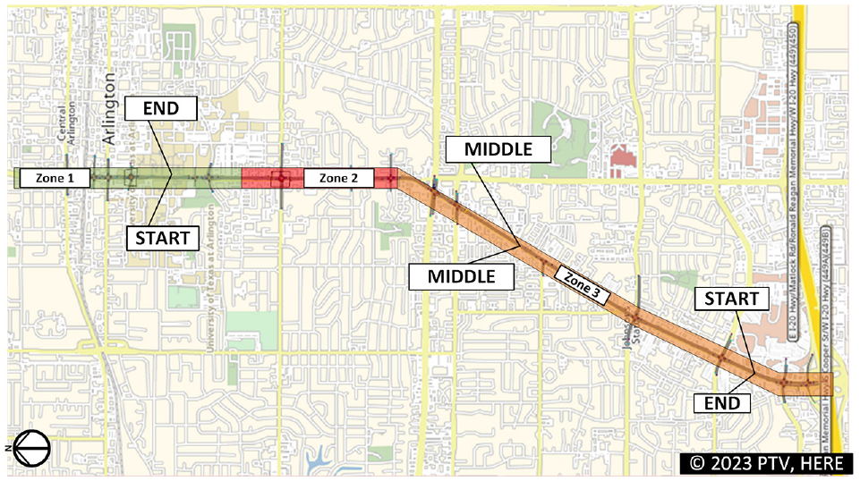
Scope and travel time collecting points along Cooper Street, Arlington, Texas.

Model Validation

Traffic volume validation: Simulated traffic volumes were first validated to compare the simulated traffic volumes and observed traffic volumes. All the intersections reveal similar validation results, and we selected one intersection to demonstrate the results. Other than the direct comparison, we also calculated the GEH value (see Figure 10b). A rule of thumb is that a GEH value of 5.0 or below indicates appropriate calibration according to the recommendation by Florida DOT and all the values were lower than that threshold.

Figure 10.

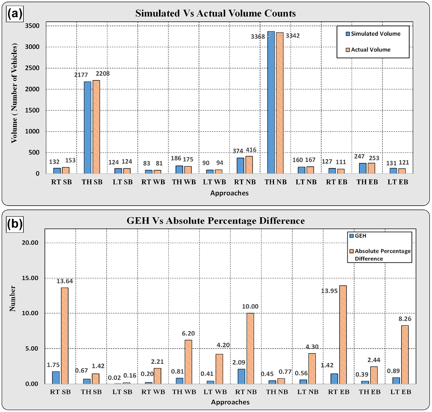
Volume validation: (a) and GEH calculation (b) (Cooper Street at UTA Blvd, Arlington, TX).

Arterial travel speed/time validation: The arterial speed profile was obtained from the processed CV data. To ensure that the simulated average speed is within ±10 mph of the actual measured speed as adopted by many agencies, the average speed of vehicles is evaluated in three different segments of the target arterial. The “START” point is located near the UTA Blvd & Cooper intersection for the SB traffic, while the same point on the northbound is considered the “END” point for the NB traffic. The “MIDDLE” point is where the speed limit changes near Arkansas Road and Cooper Street. The “END” point is located at the intersection near the I-20 interchange at Cooper Street for the SB traffic. It is also the “START” point for the NB traffic. Figure 9 shows the travel time collecting point on Cooper Street.

The simulated arterial travel speeds were summarized and then compared with the corresponding observed travel speeds from the CAV data in Figure 11, a and b . It displays the average time–mean speed at the start, middle, and end points and the time–mean speeds at three locations observed from the CV data.

Figure 11.

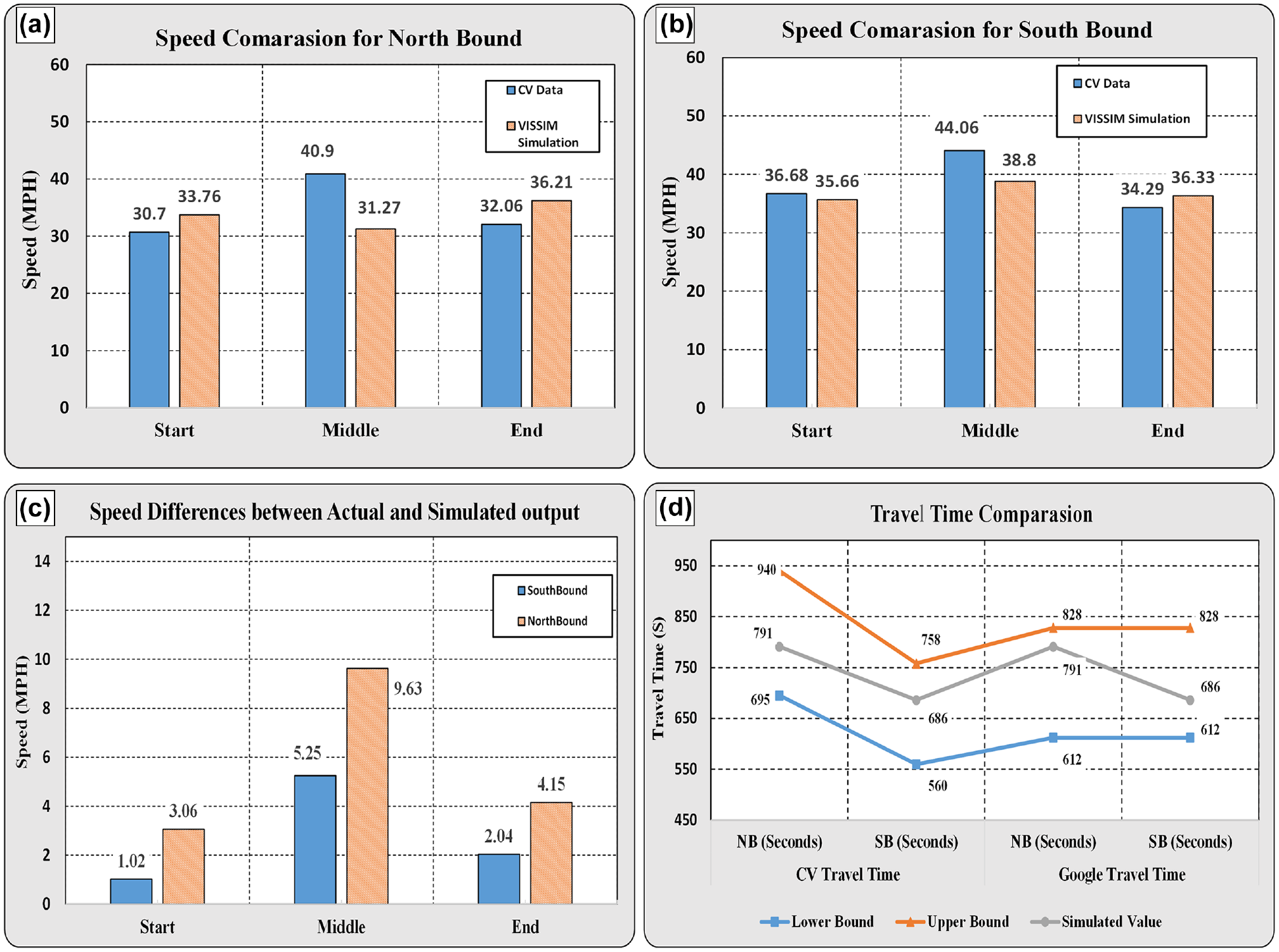
Model validation: (a) Northbound speeds, (b) Southbound speeds, (c) Speed differences from ground truth, and (d) Travel time comparison.

Figure 11c shows the difference between the observed average speed and simulated speed. None of them exceeded the threshold of 10 mph. Thus, the VISSIM model is considered validated with respect to speed.

The next measure for calibration is travel time. We decided to take the following empirical thresholds to validate: for travel times of less than 7 min, the calibrated time should be within a range of ±1 min compared to the actual travel time; for travel times greater than 7 min, the calibrated time should be within a range of 15% compared to the actual travel time.

The CV data set was used to obtain the realistic travel time and the average travel time was 533 s for end-to-end NB traffic and 585 s for end-to-end SB traffic. Figure 11d shows the upper and lower bounds of the accepted travel time. The average simulated travel time for the NB vehicles was 791 s, and it was 686 s for the SB vehicles. Both simulation results fell within the acceptable range of travel time errors. The travel time of the simulation model was also validated.

Traffic Signal Performance Evaluations in the ATSPM Systems

The simulation scenario is set as the morning peak hours: 7:30–9:30 a.m. on a typical workday when the traffic volumes and the corresponding signal timing plans are available from the City of Arlington. The VISSIM model is set to output individual records of vehicles’ trajectories, traffic signal phase transitions, and detector actuation across all 16 intersections. These simulation events need to be further parsed to be recognized by real-world ATSPM systems.

Simulated Data Parsing

Parsing vehicle trajectories: There are two challenges in parsing vehicle trajectories. The simulated vehicle trajectories are recorded at 10 Hz, whereas the real-world vehicle trajectories can only be collected once per second or multiple seconds. This constraint is governed by the GPS in reality. Therefore, the first step is to downsample the original vehicle trajectories to 1 Hz. The second step is to transform each simulation vehicle’s position from the simulated coordinates (x, y) to the WGS84 coordinates (i.e., latitude, longitude).

Parsing traffic signal events: To make traffic signal events recognizable by the UDOT ATSPM systems and UTAIM, the signal event must comply with the ATSPM data standards defined by Indiana DOT and Purdue University ( 45 ).

After parsing the simulated data into the ATSPM databases, there is a total of 206,204 simulated traffic signal events across 16 intersections: 39,882 CV trips containing 832,882 waypoints (10% penetration rate).

ATSPM MOE Analytics

Both UDOT ATSPM and UTAIM systems can visualize many novel MOEs at intersections and the entire arterials from the simulated CV data and traffic signal logs. As a demonstration, we only present one analysis of using the ATSPM systems to identify queue spillbacks and cycle failures under over-congested traffic conditions.

Arrival-on-Green Analysis

Both UDOT ATSPM and UTAIM systems generate the “Purdue coordination diagram” (PCD) in which arrivals on green (AoGs) and green time (GT) percentage ( 43 ) are summarized to reflect the performance of traffic signal performance. Both systems reported similar AoG and GT values for the simulated time at all intersections. Figure 12 shows the PCDs generated by two ATSPM systems for the NB approach at Cooper Street at Pioneer Road, a major–major intersection with a closely spaced upstream intersection.

Figure 12.

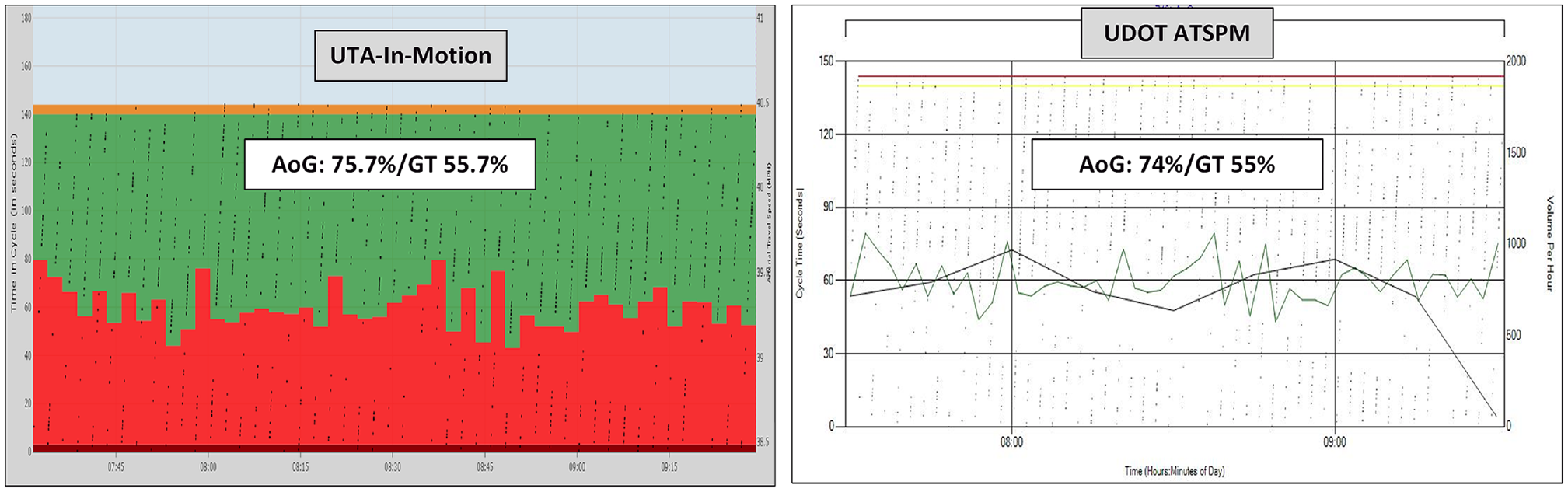
Simulated Purdue coordination diagrams generated by two automated traffic signal performance measure (ATSPM) systems.

Bottleneck Identification through “Ground Truth” Time–Space Diagram Analysis

From the traffic volume and the network layout, as well the simulation’s animation, we are aware that the NB approach at the same intersection has queue spillbacks and cycle failures. However, the values of AoG and GT imply a contradiction, as they are very high. The initial speculation is that the advance detectors are occupied by long queues so they cannot report new arriving vehicles (arriving during red) until the queue is cleared (reached the detector during green). To confirm this validation, we use the UTAIM system to generate a time–space diagram superposed with synchronous vehicle trajectories, as shown in Figure 13. After a close look at the NB approach at that intersection, we found many vehicles had to stop in queues multiple times before crossing the intersection. This is a classic sign of cycle failures. The location of the advanced detectors is relatively close to the stop bar (less than 100 ft). As a result, most vehicles will not be captured when they arrive during the red and join the queue end. These vehicles will not be captured until they begin to move during the green and the queue begins to be cleared. As a result, they will be reported as vehicles arriving on green, making the AoG values over-estimated. To address this issue, it will be necessary to place the advance detector further to accommodate long queues or combine the strength of the PCD and the time–space diagram. The location of advanced detectors can be recommended according to the simulation results.

Figure 13.

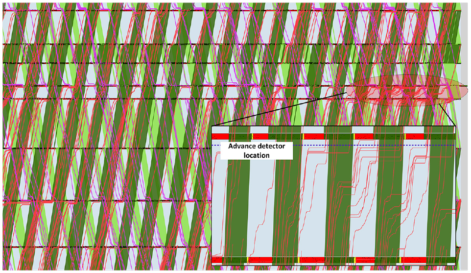
“Ground truth” time–space diagram and bottleneck analysis.

The entire system does not need large computing resources to perform. The output of each simulation to evaluate a future scenario includes 2–3 peak hours of vehicle trajectories and traffic signal control events at 10–20 intersections. During the experiments in the laboratory, the VISSIM simulation software, the UDOT-ATSPM system, UTAIM, and accompanying software were all hosted on one computer with 48 CPU cores and 256 GB RAM. The peak usage of CPU resources was about 25% and the highest usage of RAM was less than 30 GB. Therefore, the proposed framework can be deployed by agencies and firms using their regular computers.

Conclusions and Future Work

In this paper, we present a novel ATSPMs-in-the-loop simulation framework to introduce the concept of ATSPMs in the traffic signal design. The state-of-the-art ATSPM system can provide forensic analytics to the traffic signal systems for traffic signal operations while it is by default impossible to be applied to traffic signal design because the ATSPM system is data-driven, whereas most traffic signal design is for future scenarios that do not have traffic signal data yet. Inconsistency between traffic signal design and traffic signal operation will generate many issues, especially when traffic signal systems contain multimodal operations or accommodate congestion. The presented work in this paper addresses these issues by offering two benefits: visualizing ATSPM measures from traffic simulation to evaluate the proposed traffic signal performance in future scenarios and simulating the CV data and taking its strength for traffic signal performance analytics. We also describe the connected data pre-processing, simulation model calibration, and validation. In the case study, we demonstrate how to use the proposed system to identify traffic signal bottlenecks on arterials.

Next, we plan to replace the simple RBC signal emulator in the simulation model with a more advanced, full-scale signal emulator, referred to as the SILS signal emulator. The SILS signal emulator can provide realistic complex traffic signals operations, such as traffic signal priority, signal preemption, and peer-to-peer traffic coordination. The traffic signal performance under these conditions can be visualized and analyzed with the ATSPMs-in-the-loop simulation system, which will greatly facilitate traffic signal design under complex situations. We will also develop new insights on how to identify traffic signal problems based on the ATSPM digital twin.

Another novelty of the proposed ATSPM digital twin is that the employed real-world, full-scale ATSPM systems keep the same form whether they receive traffic signal data from the field or simulation. As a result, the ATSPM digital twin can also run in a “hybrid” mode in which some intersections receive simulated data while others receive real-world data for certain advanced applications. In the long term, the proposed ATSPM digital twin will be further expanded to allow other external components to interact in real-time. The appropriate components include traffic signal controller(s), the traffic signal cabinet, a cellular vehicle-to-everything (CV2X) device automated vehicle simulator, and so forth. It is possible to comprehensively evaluate real-world adaptive traffic signal systems by coupling them with the SILS in the ATSPM digital twin. It is also possible to couple traffic control hardware and real-world advanced transportation management systems (ATMSs) to provide full-spectrum training for the future workforce. It can also be coupled with other simulation and emulation systems for different purposes.

Footnotes

Author Contributions

The authors confirm contribution to the paper as follows: simulation modeling and calibration: S. Khadka; writing: S. Khadka; ATSPM systems installation and calibration: P. (Slade) Wang; system development: P. (Taylor) Li; model calibration: P. (Taylor) Li; proofreading: P. (Taylor) Li; writing the parsing software package to couple VISSIM and multiple ATSPM systems: P. (Taylor) Li; idea development: S.P. Mattings; proofreading: S.P. Mattings. All authors reviewed the results and approved the final version of the manuscript.

Declaration of Conflicting Interests

The author(s) declared no potential conflicts of interest with respect to the research, authorship, and/or publication of this article.

Funding

The author(s) disclosed receipt of the following financial support for the research, authorship, and/or publication of this article: This study was sponsored by TxDOT under Project No. 0-7160 and supported by the City of Arlington, Texas. The connected vehicle data was distributed by Wejo Data Inc.

ORCID iDs

Swastik Khadka

Peirong (Slade) Wang

Pengfei (Taylor) Li

Stephen P. Mattingly

Any opinions, findings, conclusions, or recommendations expressed in this material are those of the authors and do not necessarily reflect the official views or policies of the above organizations, nor do the contents constitute a standard, specification, or regulation of these organizations.

References

PTV VISSIM 10 User Manual. PTV AG, Karlsruhe, Germany2010.

Chowdhury

F. R.

Wang

Imtiaz

S. M.

Actuated Traffic Signal Performance Evaluation Along Arterials Using Wi-Fi Travel Time Samples and High-Resolution Traffic Signal Events Data. Transportation Research Record: Journal of the Transportation Research Board, 2020. 2674: 268–280.

Wunderlich

K. E.

Vasudevan

Wang

TAT Volume III: Guidelines for Applying Traffic Microsimulation Modeling Software 2019 Update to the 2004 Version. Federal Highway Administration, Washington, D.C., 2019.

FHWA. U.S. Department of Transportation. Transportation Systems Simulation Manual. 2020.

Why Choose Wejo. Wejo. https://www.wejo.com/why-wejo. Accessed July 30, 2023.

Khadka

Wang

P. S.

P. T.

Torres

A New Framework for Regional Traffic Volumes Estimation with Large-Scale Connected Vehicle Data and Deep Learning Method. Journal of Transportation Engineering, Part A: Systems, Vol. 149, No. 4, 2023, p. 04023015.

Ahmad

Ali

Ahmed

H. U.

Huang

Evaluating Traffic Operation Conditions During Wildfire Evacuation Using Connected Vehicles Data. Journal of Fire, Vol. 6, No. 5, 2023, p. 184.

Transforming Mobility Worldwide By Connecting People, Vehicles, Cities, and Businesses. INRIX. https://inrix.com/about/. Accessed July 30, 2023.

Why Streetlight: Our Data. StreetLight Data. https://www.citationmachine.net/apa/cite-a-website/new. Accessed July 30, 2023.

10.

Driving Directions, Traffic Reports & Carpool Rideshares by Waze. Waze. https://www.waze.com/company. Accessed July 30, 2023.

11.

NEMA Standards Publication TS 2-2021. National Electrical Manufacturers Association, Rosslyn, VA, 2021.

12.

Kazenmayer

Ford

Zhang

Rahman

Cimen

Turgut

Hasan

Traffic Volume Prediction with Automated Signal Performance Measures (ATSPM) Data. Proc., 2022 IEEE Symposium on Computers and Communications (ISCC), Rhodes, Greece, IEEE, New York, 2022, pp. 1–6.

13.

Jin

P. J.

Zhang

Brennan

T. M.

Jr. Jalayer

Real-Time Signal Performance Measurement (RT-SPM). Department of Transportation. Federal Highway Administration, Washington, D.C., 2019.

14.

Chamberlin

Fayyaz

Using ATSPM Data for Traffic Data Analytics. Department of Transportation. Research Division, Salt Lake City, UT, 2019.

15.

Remias

S. M.

Waddell

Klawon

Yang

Signal Performance Measures Pilot Implementation. Michigan Department of Transportation. Research Administration, Lansing, MI, 2018.

16.

Mathew

J. K.

Saldivar-Carrranza

Duffy

Bullock

D. M.

Integrated Performance Measures for Bus Rapid Transit System and Traffic Signal Systems Using Trajectory Data. Journal of Transportation Technologies, Vol. 12, No. 4, 2022, pp. 833–860.

17.

Jackson

Huang

Koonce

Burkman

Use of High-Resolution Signal Controller Data to Measure Transit Signal Priority Performance: A Case Study in the Boston Region. Transportation Research Record: Journal of the Transportation Research Board, 2023. 2678: 138–149.

18.

Tahsin Emtenan

Day

C. M.

Correlation Analysis for Exploring the Relationship Between Probe Vehicle Data and Event-Based Traffic Signal Performance Measures. Transportation Research Record: Journal of the Transportation Research Board, 2022. 2676: 587–600.

19.

Day

C. M.

Sturdevant

J. R.

Bullock

D. M.

Data-Driven Ranking of Coordinated Traffic Signal Systems for Maintenance and Retiming. Transportation Research Record: Journal of the Transportation Research Board, 2018. 2672: 167–178.

20.

O’Brien

Stevanovic

Day

Hale

Matout

A Methodology and Case Study: Evaluating the Benefits and Costs of Implementing Automated Traffic Signal Performance. United States. Federal Highway Administration, Reston, VA, 2020.

21.

Day

C. M.

Bullock

D. M.

Optimization of Traffic Signal Offsets with High Resolution Event Data. Journal of Transportation Engineering, Part A: Systems, Vol. 146, No. 3, 2020, p. 04019076.

22.

Emtenan

A. T.

Day

C. M.

Impact of Detector Configuration on Performance Measurement and Signal Operations. Transportation Research Record: Journal of the Transportation Research Board, 2020. 2674: 300–313.

23.

Dumitru

A. M.

Assessing the Impact of School Bus Traffic Using Modeling Software and Automated Traffic Signal Performance Measures. The University of North Carolina, Charlotte, 2019.

24.

Park

Schneeberger

Microscopic Simulation Model Calibration and Validation: Case Study of VISSIM Simulation Model for a Coordinated Actuated Signal System. Transportation Research Record: Journal of the Transportation Research Board, 2003. 1856: 185–192.

25.

Ostojic

Jolovic

Stevanovic

Building, Calibrating, and Validating a Large-Scale High Fidelity Microscopic Traffic Simulation Model-A Manual Approach. Proc., 95th Annual Meeting of the Transportation Research Board, Washington, D.C., 2016.

26.

Stevanovic

Martin

Optimizing Signal Timings from the Field: VISGAOST and VISSIM–ASC/3 Software-in-the-Loop Simulation. Transportation Research Record: Journal of the Transportation Research Board, 2009. 2128: 114–120.

27.

Aghabayk

Sarvi

Young

Kautzsch

A Novel Methodology for Evolutionary Calibration of Vissim by Multi-Threading. Australasian Transport Research Forum, Vol. 36, No. 1, 2013, pp. 1–15.

28.

Chen

Wan

Guo

Calibration of VISSIM for Bus Rapid Transit Systems in Beijing Using GPS Data. Journal of Public Transportation, Vol. 9, No. 3, 2006, pp. 239–257.

29.

Abduljabbar

Dia

Liyanage

Bagloee

S. A.

Applications of Artificial Intelligence in Transport: An Overview. Sustainability, Vol. 11, No. 1, 2019, p. 189.

30.

Sun

D. J.

Zhang

Chen

Comparative Study on Simulation Performances of CORSIM and VISSIM for Urban Street Network. Simulation Modelling Practice Theory, Vol. 37, 2013, pp. 18–29.

31.

Menendez

Sensitivity Analysis for Calibrating Vissim in Modeling the Zurich Network. Paper Presented at the 12th Swiss Transport Research Conference, Ascona, Switzerland, 2012.

32.

Cascetta

Transportation Systems Analysis: Models and Applications. Springer Science & Business Media, Napoli, Italy, 2009.

33.

Hellinga

B. R.

Requirements for the Calibration of Traffic Simulation Models. Proceedings of the Canadian Society for Civil Engineering, Vol. 4, 1998, pp. 211–222.

34.

Seshadri

Azevedo

C. L.

Ben-Akiva

M. E.

Demand Calibration of Multimodal Microscopic Traffic Simulation using Weighted Discrete SPSA. Transportation Research Record: Journal of the Transportation Research Board, 2019. 2673: 503–514.

35.

Maheshwary

Bhattacharyya

Maitra

Boltze

A Methodology for Calibration of Traffic Micro-Simulator for Urban Heterogeneous Traffic Operations. Journal of Traffic Transportation Engineering, Vol. 7, No. 4, 2020, pp. 507–519.

36.

Bartin

Ozbay

Gao

Kurkcu

Calibration and Validation of Large-Scale Traffic Simulation Networks: A Case Study. Procedia Computer Science, Vol. 130, 2018, pp. 844–849.

37.

Khadka

P. T.

Wang

Developing Novel Performance Measures for Traffic Congestion Management and Operational Planning Based on Connected Vehicle Data. Journal of Urban Planning, Vol. 148, No. 2, 2022, p. 04022016.

38.

Wiedemann

Simulation des Strassenverkehrsflusses. Institut für Verkehrswesen der Universitüt Karlsruhe, Karlsruhe, 1974.

39.

Fellendorf

Vortisch

Validation of the Microscopic Traffic Flow Model VISSIM in Different Real-World Situations. Presented at 80th Annual Meeting of the Transportation Research Board, Vol. 11, Washington, D.C., 2001.

40.

Zhou

Bakshi

Prasanna

Soma

Towards an Integrated Modeling and Simulation Framework for Freight Transportation in Metropolitan Areas. Proc., 2008 IEEE International Conference on Information Reuse and Integration, Las Vegas, NV, IEEE, New York, 2008, pp. 280–285.

41.

FDOT. Traffic Analysis Handbook. Florida Department of Transportation, Tallahassee, FL, 2014.

42.

WisDOT. Microscopic Simulation Traffic Analysis. Traffic Engineering, Operations & Safety ManualTraffic Engineering, Operations & Safety Manual, Wisconsin Department of Transportation, Madison, WI, 2019.

43.

Park

Development and Evaluation of a Procedure for the Calibration of Simulation Models. Transportation Research Record: Journal of the Transportation Research Board, 2005. 1934: 208–217.

44.

Jie

Van Zuylen

Chen

Viti

Wilmink

Calibration of a Microscopic Simulation Model for Emission Calculation. Transportation Research Part C: Emerging Technologies, Vol. 31, 2013, pp. 172–184.

45.

Sturdevant

J. R.

Overman

Raamot

Deer

Miller

Bullock

D. M.

Day

C. M.

Brennan

T. M.

Jr. Li

Hainen

Indiana Traffic Signal Hi Resolution Data Logger Enumerations. Indiana Department of Transportation and Purdue University, West Lafayette, 2012, p. 13.

Automated Traffic Signal Performance Measures (ATSPMs) in the Loop Simulation: A Digital Twin Approach

Abstract

Keywords

Literature Review

Emerging Traffic Big Data for Traffic Signal Systems

Automated Traffic Signal Performance Measures

Simulation Model Calibration

Automated Traffic Signal Performance Measures-in-the-Loop Simulation Framework

Connected Vehicle Data Processing

Data Reduction and Processing for Regions of Interest

Microscopic Simulation Modeling

Network Construction

Simulation Calibration

Countable Measure Calibration

Behavioral Measure Calibration

Case Study: Bottleneck Identification using Automated Traffic Signal Performance Measures along Cooper Street in Arlington, Texas

Model Validation

Traffic Signal Performance Evaluations in the ATSPM Systems

Simulated Data Parsing

ATSPM MOE Analytics

Arrival-on-Green Analysis

Bottleneck Identification through “Ground Truth” Time–Space Diagram Analysis

Conclusions and Future Work

Footnotes

Author Contributions

Declaration of Conflicting Interests

Funding

ORCID iDs

References