Sage Journals: Discover world-class research

Abstract

This paper considers which work-related trip patterns are included in household travel surveys and which in commercial travel surveys and if there are certain patterns that are distinctly underrepresented in either one. The study is structured as a comparison between data from a household travel survey and data from a commercial travel survey. Both surveys were conducted in Germany and within close temporal proximity. We applied cluster analysis to identify differences in the data and identify work-related travel patterns. The results show that work-related travel patterns are quite complex. Although some patterns are covered in both surveys, mobile workers’ travel patterns in particular are not represented well in the household travel survey. Furthermore, our analysis shows that not all commercial trips are generated by motorized vehicles and a considerable share of work-related trips are undertaken using public transport or active modes of transport that are not covered by the commercial travel survey. The results indicate that researchers and transport planners creating travel demand models need to pay more attention to work-related travel behavior and acknowledge that depending on the area of study, traditional household travel surveys may not provide a complete sample of the population; however, simply adding data on commercial trips from commercial travel demand models to data from household travel surveys does not provide a complete picture of work-related travel either.

Keywords

data and data science commercial vehicle survey planning and analysis forecasts/forecasting trip generation modeling household travel surveys travel surveys travel pattern work-related transport

To this day, travel behavior analyses and travel demand models still rely on data from household travel surveys (HTSs). Although information and communications technology and especially global navigation satellite system technology have simplified the survey process in some cases, many traditional and nationwide travel surveys still rely on manual input. In these cases, the issue of underreporting trips is more of a problem because there are no mechanisms to validate trip characteristics such as number, start times, and distances. Previous research shows that work-related trips have been affected by this underreporting for a long time. In 1990, Brög and Winter ( 1 ) investigated the problem of unreported commercial trips in HTSs and have identified a correction factor of 2.0 for work-related trips. This means that for each reported work-related trip in a HTS, in actuality, twice as many trips were undertaken ( 1 ). Albeit more recent studies show less drastic factors of underrepresentation, they confirm the issue of underreporting work-related trips in HTSs. Itsubo and Hato ( 2 ) compared the results of a GPS-based travel survey with those from a paper-based survey. They found that more work-related trips were reported in the GPS-based survey than in the paper-based one. This holds true when considering both all modes of transport and cars only. Itsubo and Hato ( 2 ) and Stopher et al. ( 3 ) presented similar findings with regard to work-related trips. In their work, they assessed the accuracy of the Sydney HTS with a GPS survey. Although the small number of missed trips is too small for them to conclude significant effects, the surveys did not differentiate between work-related and commuting trips ( 3 ). However, routine trips, such as commuting trips, are less likely to be underreported ( 2 ); thus, in relation to work trips as a combination of commuting and work-related trips may have skewed the results. To gain more information on commercial transport, several surveys have been conducted to account specifically for work-related trips. Although they have provided further insights with regard to these trips they cannot be considered as completely supplemental because an overlap in information can be expected.

This paper investigates which work-related trip patterns are included in HTSs and commercial travel surveys (CTSs) and if there are certain patterns that are distinctly underrepresented in either one. In this study, work-related trip patterns are considered on an individual level and cover all trips that were undertaken in the course of the respondents’ work. In this case, commuting trips were not regarded as work-related trips. This study is structured as a comparison between data from a traditional HTS and that from a CTS. Both surveys were conducted in Germany and within close temporal proximity. We applied cluster analysis to increase our understanding of differences in data and identify work-related travel patterns. Recognizing that results of cluster analyses are often ambiguous, this study aims to provide general indications of the coverage of the different surveys in relation to work-related trip patterns, and identify gaps and redundancy in data.

Identifying which travel patterns might be missing in surveys can be difficult, because in most cases, work-related variables—be they travel purpose or workplace information—are only considered in scant detail. However, commercial travel is just as complex as its private counterpart. For example, tradespeople tend to make trips with several different purposes: service to a customer; transportation of material to a construction site; shopping trip to purchase material. Although these different purposes and professions entail different behavioral travel patterns, traditional HTSs only account for these trips using a single trip purpose (work) and very broad categorizations of work status (full-time, part-time, unemployed) (see, for example [4 –7]). The problem of the scant detail with regard to occupational information and work-related trip data also becomes apparent when analyzing working-from-home behavior. Telecommuting and remote work have been considered as a solution for peak-hour traffic congestion for over four decades, because working from home reduces the number of vehicle miles traveled (VMT) during commuting trips (see e.g., [8 –15]). However, not everybody can work from home because not every job can be carried out remotely ( 16 , 17 ); thus, work-related travel will continue to contribute to traffic loads.

Previous studies have identified several different influencing factors with regard to work-related travel. For example, Mohino et al. ( 18 ) find there is a significant difference between people’s work-related travel behavior depending on their level of education. Although this and other studies (e.g., Beaverstock and Budd [ 19 ], Jeong et al. [ 20 ]) focus on business travel, especially with regard to overnight stays made by professionals and managers, Hislop ( 21 ) highlights the significance of analyzing nonmanagerial mobility patterns. He determined that managerial and professional workers show a distinctly different mobility pattern compared with workers such as engineers and construction site project managers who can be a lot more mobile.

In addition to the influence of occupation on work-related travel, previous studies have also identified the relationship between company characteristics and work-related trip generation. Steinmeyer and Wagner ( 22 ) estimate the commercial service trip generation for the city of Berlin based on company information such as industry sector, size, and vehicle fleet. Hebes et al. ( 23 ) identified further influencing factors on work-related trips such as the location of the customer when a service trip is undertaken. Both a company’s location and the number of customers have been identified as determining its trip generation rate ( 24 ). Furthermore, previous studies showed that the required tools and resources at the job site, for example, machines or computers, influence trip chaining behavior and travel mode choice ( 25 , 26 ).

To increase insights into work-related travel patterns, there have been several efforts to gather information on commercial transport that have focused on light commercial vehicles. Hunt et al. ( 27 ) conducted a survey of commercial vehicles in Edmonton and Calgary, Canada and found that about 12% of VMT are attributed to commercial movements, that is, work-related travel. They differentiated between goods stops, service stops, transport handling stops, and other stops. In both cities, about 35% of stops are made to provide a service. Similar examples of CTSs include smaller establishment-based surveys ( 28 ) and large-scale surveys ( 29 ) conducted in Germany. These surveys provide much more detail and have proved to be suitable for commercial travel demand modeling. Based on the survey conducted in Canada ( 27 ), Stefan et al. ( 30 ) and Hunt and Stefan ( 31 ) developed a microscopic simulation model of commercial vehicle movements that was later extended and transferred to Ohio, U.S.A. ( 32 ) and the Greater Toronto and Hamilton Area in Canada ( 33 ). Another model of commercial transport was developed for Sydney, Australia ( 34 ). In previous works, we have presented a microscopic demand model of commercial transport in Germany ( 35 , 36 ). Both CTSs and the travel demand models based on these provide much needed information and insights into commercial travel behavior. The advantage is that these models are capable of simulating the complex work-related trip chains ( 37 ). However, on the one hand, they are often developed independently of existing data sources (i.e., traditional HTSs) and travel demand models. On the other hand, traditional HTSs and travel demand models often include work-related trips; thus, superposition of the results does not work, because both types of model include some work-related transport.

In the following section, we explain the data used for the analysis, including its preparation and descriptive analysis. We continue by describing the multivariate analysis method used (cluster analysis). The results section of the paper contains the outcome of our analyses, which we discuss in the subsequent section. The conclusion of this paper addresses the main outcomes of our work and its implications.

Materials and Methods

This study relies on two main sources of data: HTS and CTS. We describe these data and their processing below.

Data

To capture commercial travel patterns, the German Federal Ministry of Transport and Digital Infrastructure commissioned the nationwide vehicle-based travel survey Motorized Transport in Germany (Kraftfahrzeugverkehr in Deutschland [KiD]). Recognizing that there are existing statistics and data sources in relation to freight traffic created by larger vehicles, KiD focused on light vehicle commercial travel. The data is divided into four different data sets: vehicle data, trip data, trip chain data, and geospatial data. KiD was carried out in 2002 and 2010. The sample of KiD 2010, which we used as a database for our analyses of commercial trips, includes data on 70,249 vehicles, and on the survey day, 177,377 trips were undertaken with these vehicles ( 29 ).

As a proxy for traditional HTSs we used data from Mobility in Germany (Mobilität in Deutschland [MiD]). MiD is a nationwide HTS commissioned by the German Federal Ministry of Transport and Digital Infrastructure with the purpose of capturing households’ daily travel behavior. Respondents were asked to report generic household information and their travel behavior using a travel diary for one day. MiD was conducted in 2002, 2008, and 2017. Although choosing the most recent data is generally sensible, we have opted to use MiD 2008 for two reasons: it is temporally closer to KiD 2010, which allows for a more stable comparison; and MiD 2008 contains a section on regular work-related trips. MiD 2008 is comprised of four different data sets: car data, household data, person data, and trip data. For this study, we used the base sample, which includes information on 25,922 households, 60,713 persons, 193,290 trips, and 34,601 cars ( 38 ).

Data Preparation

Although the HTS and CTS data sets share characteristics, they are not comparable without adjustments. For our analysis, we first had to choose variables and then prepare and merge the data accordingly. Because our goal is to identify travel patterns, we used trip-related data. With regard to the CTS, both the trip and the trip chain data sets include trip-related information. Although the trip chain data set includes fewer variables, they are already grouped by vehicle and summarize all relevant characteristics of the trip chains: cumulative travel time, cumulative activity duration, time of first work-related trip, cumulative trip distance, and number of stops. The data already come in a prepared format, but there are a lot of missing values (see Table 1), the variable with the most missing values being activity duration. Although we recognize that this variable might have high explanatory value, we chose to exclude it from subsequent analyses because we would have lost too many observations. Imputation was not suitable either, because we would have had to use the same variables for imputation and cluster analysis. This would have resulted in biased results. Rather, we imputed activity duration and analyzed this variable after conducting the cluster analysis. Although cumulative travel time does not present as many missing values as activity duration, we opted not to use this variable either because of its correlation with the variable cumulative trip distance, because the cluster analysis would again have been biased by using correlated variables. Subsequently, we removed entries that were missing time of first trip and cumulative trip distance, resulting in 27,306 observations.

Table 1.

Summary Statistics of CTS and HTS

	Start of first trip		Trip duration		Trip distance		Number of trips		Activity duration
	CTS	HTS	CTS	HTS	CTS	HTS	CTS	HTS	CTS	HTS
Min.	0.00	0.00	1.00	1.00	0.30	0.10	1.00	1.00	1.0	0.0
1st Qu.	6.00	8.00	15.00	13.33	7.57	3.80	2.00	1.00	120.0	190.0
Median	7.00	9.00	29.55	25.50	17.10	10.69	2.00	2.00	292.5	390.0
Mean	7.67	10.43	65.49	47.83	62.26	40.07	4.24	2.15	296.8	431.8
3rd Qu.	8.00	13.00	57.50	53.00	49.00	31.35	4.00	3.00	470.0	630.0
Max.	23.00	23.00	3960.00	480.00	1800.00	722.00	343.00	10.00	1020.0	2379.0
NA	130	0	8,171	0	241	0	0	0	25,377	0

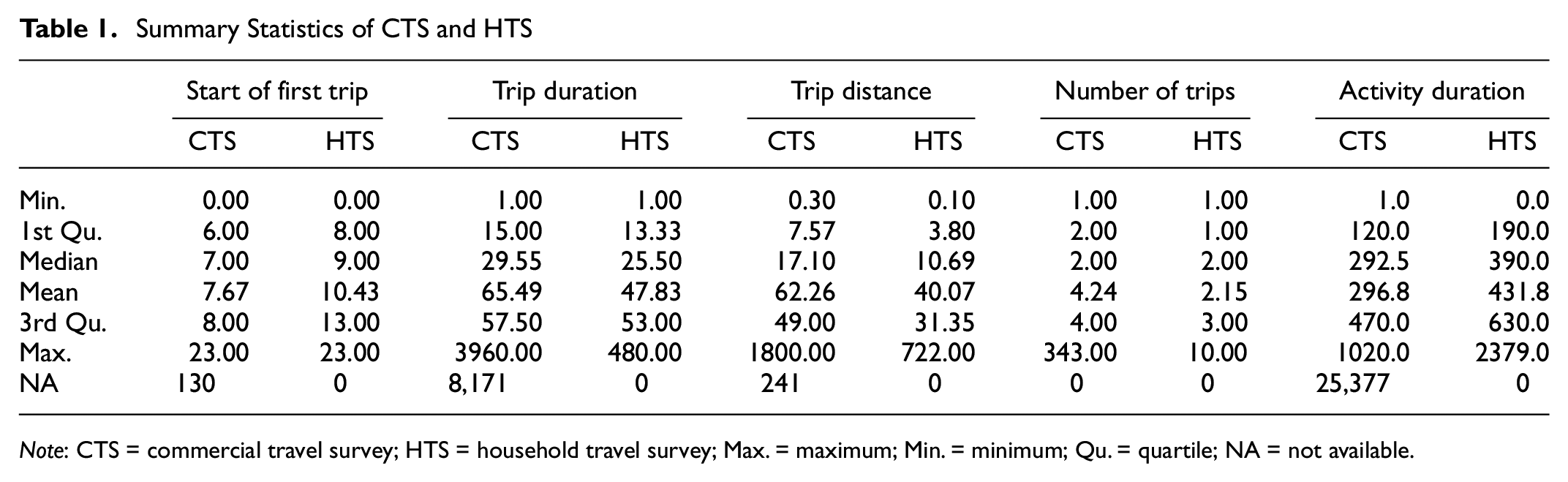
Note: CTS = commercial travel survey; HTS = household travel survey; Max. = maximum; Min. = minimum; Qu. = quartile; NA = not available.

According to the chosen variables in the CTS, we selected the corresponding variables in the HTS. For this step, we selected only work-related trips and determined the start of the first trip. We then grouped the data by respondent and summarized distances traveled and number of stops. This resulted in 1,222 observations. After this step, we were able to merge the data from both data sets into one large data set with 28,528 observations, and this is the data set used in the following analysis.

Descriptive Analysis

To gain a better overview of the data sets and to identify differences in variables, we first present a descriptive analysis of the individual variables of the two data sets. The data for trip-related variables are presented in Table 1. For variables with missing values, the statistics are based on the available values. Therefore, they do not necessarily represent the sample.

The analysis shows that the first trip of the day in the CTS tends to start earlier than the first trip in the HTS. The median start time of the first trip in the CTS is 7 a.m. whereas the first trip of the day in the HTS has a median of two hours later. Whereas the median cumulative trip duration (in minutes) of CTS trips is quite close to those in the HTS, the CTS includes temporarily longer trip chains. The same holds true for the variable cumulative trip distance (in km). The CTS includes longer trips and the median cumulative trip distance is also 6.5 km longer. The reported median number of trips per respondent is the same in both surveys, whereas the mean is twice as high in the CTS. Furthermore, the CTS includes trip chains with up to 343 trips, which is over 30 times higher than the number of trips included in the HTS. Although the CTS includes shorter activities, compared with HTS activities durations are longer.

Cluster Analysis

To identify travel patterns with regard to work-related trips and analyze differences between traditional HTS data and designated CTS data, we used cluster analysis.

Cluster analysis is a method of pattern recognition to find groups in a population comprised of individuals. It works by increasing the similarity within a group and the dissimilarity to other groups ( 39 ). Although cluster analysis is a powerful tool for exploratory data analysis, its use is only warranted if there is a cluster structure present in the data. To determine whether cluster analysis would be appropriate in our case, we performed multiple multimodality tests on our data. Multimodality tests are based on the notion that if the data are structured in clusters, there should be some differences in clusters, for example, in the histogram of pairwise distances, whereas homogeneous data that have no underlying cluster structure will not show such differences. Multimodality tests generally assume that the data have no structure as per the null hypotheses, and if the data can be clustered, this hypothesis is refused ( 40 ). To evaluate the clusterability of our data, we performed those tests that Adolfsson et al. ( 40 ) identified as suitable for multidimensional data: the dip test on pairwise distances ( 41 ); the dip test on the first principal component ( 40 ); and the Silverman test ( 42 ) on the first principal component ( 43 ). The results of all three tests indicated that the data we proposed to use for the cluster analysis were suitable for the approach.

There are many different clustering methods and the choice is highly dependent on the objective of the study and the available data. Cluster analysis methods can broadly be split into three groups: probabilistic and generative models; distance-based; and density-based ( 44 ). In our case, we did not have labels in the data and we did not want to make a priori assumptions about the number of clusters. We also wanted the individuals grouped together to be as similar as possible. Because probabilistic models require information on the underlying distribution of the data, and density-based models such as DBSCAN (density-based spatial clustering of applications with noise) require knowledge of the density of the data to determine a sensible radius and minimum number of points in each cluster, we could only consider distance-based methods. Distance-based clustering methods can be categorized further into partitional and hierarchical models. In partitional cluster analysis, the analyst first has to determine prototype points for each cluster around which the subsequent partitions of data are formed. Again, the requirement for input before the analysis disqualifies this method. This initial input is generally not necessary for hierarchical clustering methods, which group data points based on their distance.

In this study, the objective was to obtain stable clusters with a small within-cluster variance. A suitable criterion for this objective is Ward’s method. We conducted the cluster analysis in R using the stats package ( 45 ). The package provides a function called hclust, in which the most common hierarchical clustering algorithms are implemented. To account for the variables which are measured in different units (time, distance, absolute numbers), we first needed to scale the data. Otherwise, cumulative trip distance, for example, would be weighted higher in the analysis than the time of the first trip because their ranges of value differ substantially. After scaling the data, we used the Euclidean distance to calculate the distance matrix. This distance matrix serves as the input for the clustering analysis. As stated before, we applied Ward’s method, which is implemented in hclust as the method ward.D2 ( 46 ). The cluster analysis results in a dendrogram that is a visual representation of the points at which the clusters are merged. This serves as a basis for determining the number of clusters, because it represents the distances between different cluster solutions. A common heuristic for determining this number is the elbow criterion ( 47 ). The purpose of this method is to find a point at which increasing the number of clusters is no longer sensible because differences between clusters decrease. This point can be identified by plotting the distance between clusters over the number of clusters. Depending on the data, this may not be a definite point in the plot and sometimes multiple elbows can be identified. The elbow plot of the aforementioned cluster analysis is presented in Figure 1.

Figure 1.

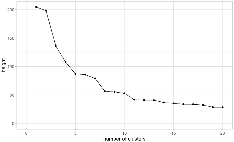
Elbow plot of Ward cluster analysis.

The graph shows that there are several possible solutions: a 5-cluster and a 8-cluster solution is sensible. To choose the final cluster model, we determined validation measures for both solutions. Generally, external and internal validation measures are differentiated. In this study, no external information is available; thus, only internal validation measures are used. Although there are several different measures available, there is no guidance on which is best ( 48 ). Therefore, we determined several of the most commonly used validation measures for both the 5- and 8-cluster solutions (see Table 2).

Table 2.

Internal Validation of Possible Cluster Solutions

measure	Value		Optimal value
measure	5 clusters	8 clusters	Optimal value
Average distance between clusters	2.4394	2.2344	Max.
Average silhouette width	0.3697	0.3449
Pearson gamma index	0.4716	0.4134
Dunn index	0.0008	0.0010
Calinski–Harabasz index	13288.66	13994.23
Separation index	0.0821	0.0566
Entropy	1.2461	1.6497	Min.
CVNN index	1.6449	1.7699	Min.

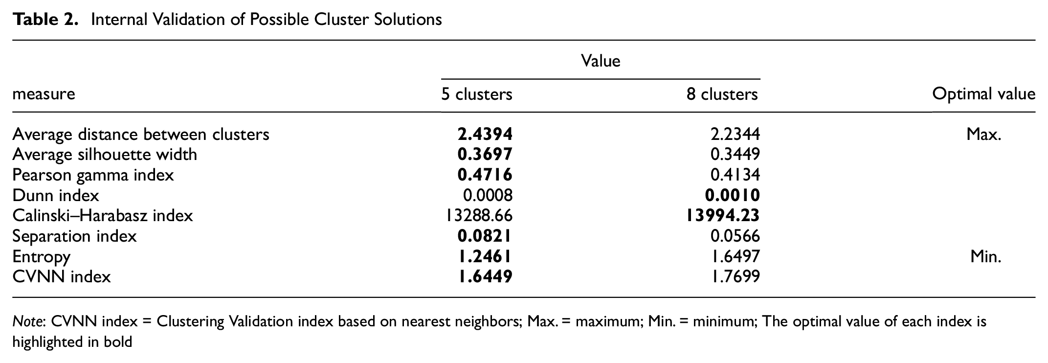
Note: CVNN index = Clustering Validation index based on nearest neighbors; Max. = maximum; Min. = minimum; The optimal value of each index is highlighted in bold

Analysis of the validation measures shows that most measures support the 5-cluster solution. Of the eight considered measures, only two support the 8-cluster solution. This ambiguity could be explained by the Dunn index, for example, not being suitable for data with sub-clusters ( 49 ). Because determining the cluster structure in the data is part of this study, we cannot make assumptions about any sub-clusters. However, the CVNN index (Clustering Validation index based on nearest neighbors) is suitable for many different kinds of data ( 48 ) and supports the 5-cluster solution. Because the majority of indices indicate that the 5-cluster solution better explains the underlying structure in the data, we have based the further analysis on this partition.

Results and Discussion

In this section we present the results of the cluster analysis. We first compare the characteristics of the different clusters with each other and then analyze which information is represented in the HTS and CTS. At the end of this section we consider the implications of our findings and provide some limitations of the study.

Cluster Characteristics

The characteristics of each cluster in the 5-cluster solution are presented in Table 3. Although all groups contain observations from the CTS, cluster 5 does not contain any observations from the HTS. Cluster 4 also includes relatively few observations from the HTS, already indicating that although the two surveys cover similar patterns, some are not present or included only to a small degree in the HTS. The largest cluster is cluster 3, with a little over half of observations falling into this group. It contains observations from both the CTS and HTS.

Table 3.

Cluster Characteristics

	Cluster 1	Cluster 2	Cluster 3	Cluster 4	Cluster 5
N	6,369	3,470	15,418	2,128	1,143
N (%)	22	12	54	7	4
CTS	5,817	3,344	14,923	2,079	1,143
CTS (%)	21	12	55	8	4
HTS	552	126	495	49	0
HTS (%)	45	10	41	4	0

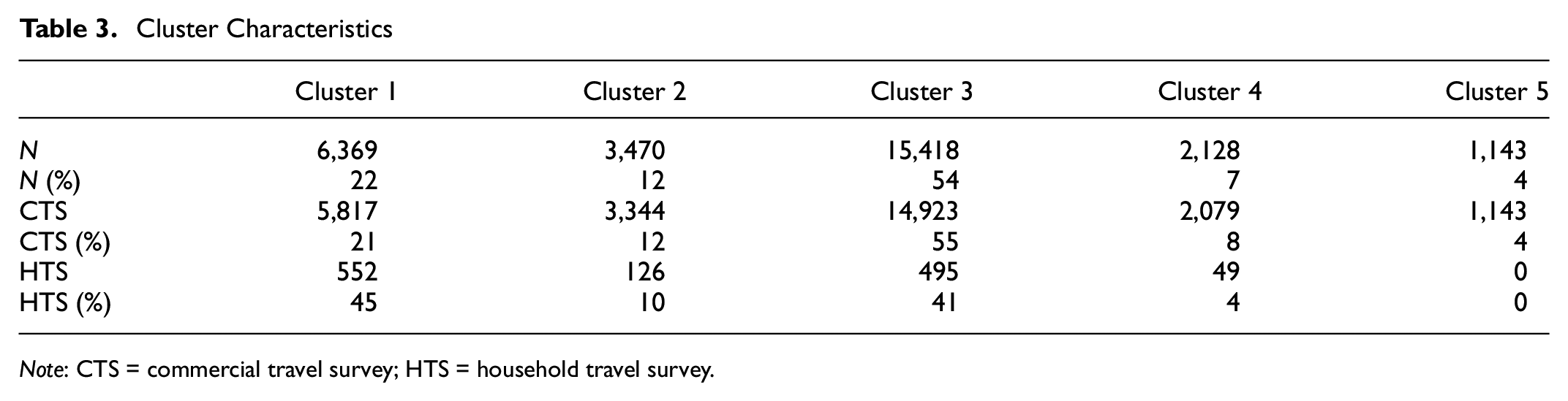
Note: CTS = commercial travel survey; HTS = household travel survey.

The characteristics of the cluster variables in the different clusters are presented in Figure 2.

With regard to cumulative trip distance, cluster 2 and cluster 4 show much higher distances than other clusters. Observations in cluster 2 result in a mean distance of 250 km and those in cluster 4 have a mean distance of 470 km. All other clusters present mean cumulative distances between 40 km and 115 km. Cluster 5 is the most distinct group considering total number of trips. Whereas all other clusters show an average number of trips below 10, observations in cluster 5 result in an average number of just over 100 trips. Considering the start of the first trip, drivers in clusters 1 and 2 do not undertake any trips at night and those in cluster 1 start their first trip comparatively late. Whereas the mean of the start time of drivers’ first trips in cluster 5 is similar to those in cluster 2, the variance is higher, especially toward the early hours of the day. Clusters 3 and 4 exceed this variance and cluster 4 especially includes patterns in which the first trip of the day is undertaken rather early.

Figure 2.

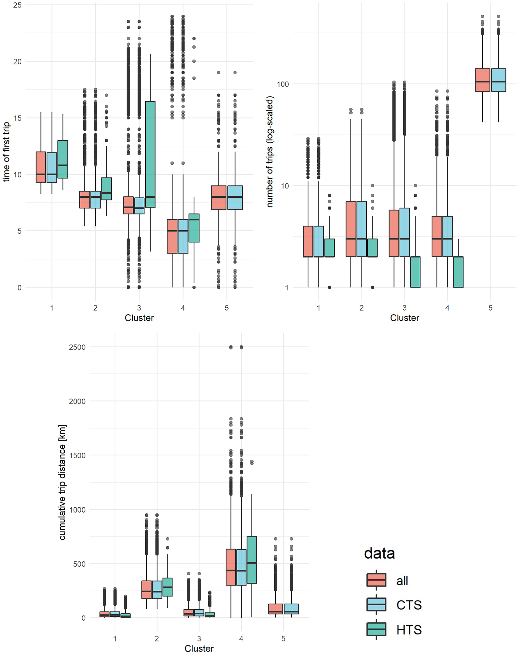
Boxplots of start time, trip distance, and number of trips.

With regard to the difference between the data sources, most clusters show similar values from both surveys and show that the different ratio of observations is generally unproblematic. The only significant deviation is the start times in cluster 3. In this cluster, the start times in the HTS vary much more across the day. Thus, this cluster is heavily influenced by the many observations from the CTS.

Subsequently, we conducted a bivariate analysis of the cluster variables, and the bivariate plots of the cluster variables are presented in Figure 3. They show that patterns including cluster 1 are those with the least variation of all variables. The start times are limited to the regular hours of a working day and neither the number of trips nor the cumulative trip distance in this cluster are particularly high, which is in accordance with the rather late start times. Because these drivers do not undertake many or long trips, they do not need to start their trips early in the day. This is opposed to cluster 2, in which start times vary much more over the course of a day with a higher cumulative trip distance. With regard to the relationship between trip distance and number of trips, drivers from cluster 2 undertake relatively few but long trips. This also holds true for cluster 4, in which this characteristic is more prevalent. Drivers in cluster 4 do not show a particular pattern with regard to the start time of the first trip. However, with regard to trip distance and number of trips, we can see that the long distances are achieved with relatively few trips. Cluster 3 is comparable with cluster 1, but with higher variable variance in all dimensions. The start times of the first trip are spread over the course of the day. Particularly for trip patterns with high cumulative trip distances and more trips, the trips start earlier in the day. Cluster 5 includes trip patterns with many trips throughout the day. This is achieved by starting relatively early in the day and by undertaking shorter trips.

Figure 3.

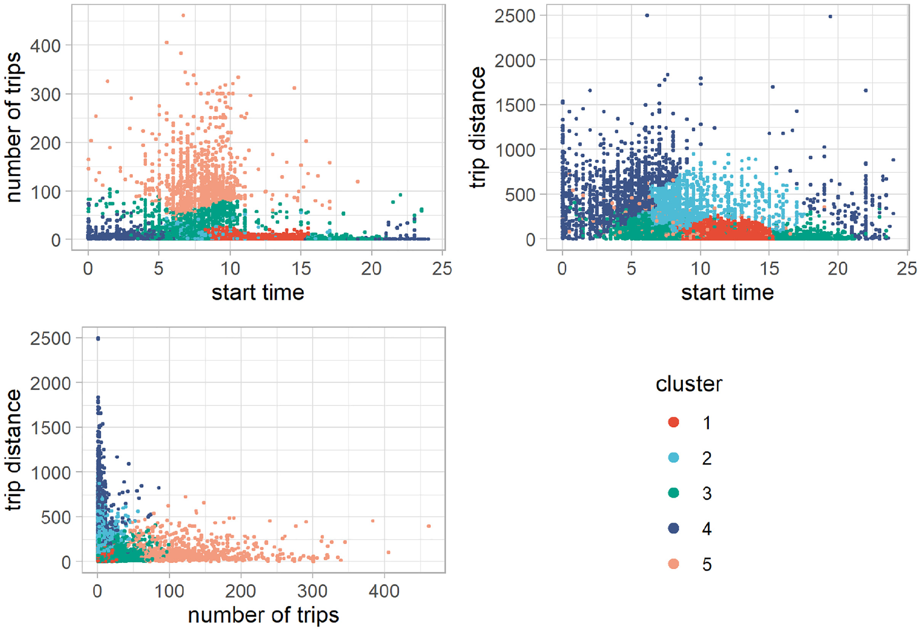
Bivariate plots colored by cluster.

Our results show that both data sets and, therefore, both survey methods capture different travel patterns. Based on the cluster characteristics, we have identified four groups with distinct work-related travel patterns: average mobile workers (cluster 3); late starters (cluster 1); long-distance travelers (clusters 2 and 4); and highly active workers (cluster 5). The groups that include two clusters all have one cluster with moderate characteristics and one with more extreme characteristics.

The average mobile workers are well represented in both surveys. They tend to start their day early in the morning, suggesting that they start their first trip from home and not from their business location. The mean cumulative trip distance of this cluster suggests that the workers stay within their own area of operation. The same is true for the late starters; however, the start hour of the first trip suggests that they start their working day at the office or location of business. Cluster 2 especially shows late start times, and although cumulative trip distances are not distinctly low, on average, workers in this cluster only undertake 2.33 trips. The long-distance clusters each have very high average cumulative trip distances, and cluster 5 does not contain any observation under 78 km. Cluster 4 has a maximum cumulative trip distance of 2,500 km. To manage such long distances, the travelers start their trips early in the day. Although they make on average more trips a day than the late starters, with an average number of trips per day of 5.17 and 4.84 respectively, these travelers do not make many trips per se. Opposed to these are the highly active workers who undertake many trips. Not only is the mean number of trips high, the minimum numbers are also considerably higher in this cluster: workers in cluster 5 make a minimum of 42 trips and as many as 462 trips a day. Although observations in this cluster show higher cumulative trip distances compared with late starters, the people concerned cannot be regarded as long-distance drivers, especially considering the high number of trips, which suggests that each trip is relatively short considering distance.

After analyzing the characteristics of the trip variables of the clusters, we further analyzed the following: activity duration of the respective trips; the sociodemographic characteristics of the workers; the characteristics of the vehicles used to undertake the trips; industry sector; and trip purposes. Because this information has missing values, we were not able to include it in the cluster analysis. However, it still provides further insights into the trip patterns represented in the different survey types.

Activity Duration

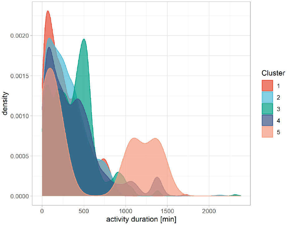
As mentioned before, we did not include activity duration in the cluster variables; however, it is still a valuable characteristic concerning trip patterns. Therefore, we opted to impute missing values and to analyze the activity duration by cluster. We tested different imputation methods and chose the one that yielded the best results when comparing observed and imputed data. We applied multivariate imputation using the R package mice ( 50 ), and yielded the best results with the predictive mean matching imputation method. The density plot of the activity duration for each cluster is presented in Figure 4.

Figure 4.

Activity duration by cluster.

The plot shows that cluster 1 includes patterns with relatively short activities. The same holds true for clusters 2 and 4, but with more variance toward longer activities. Cluster 3 has a peak of activities that last around 500 min, which is in accordance with the regular period of a working day. Somewhat ambiguous are the results concerning cluster 5: activities of a shorter duration are expected, because this cluster includes trip patterns with many trips and, therefore, many activities of short duration. However, there are a significant number of trips with subsequent activities of a very long duration that cannot be explained intuitively. One explanation could be that these observations are recorded when overnight activities are taking place.

Sociodemographic Characteristics of Workers

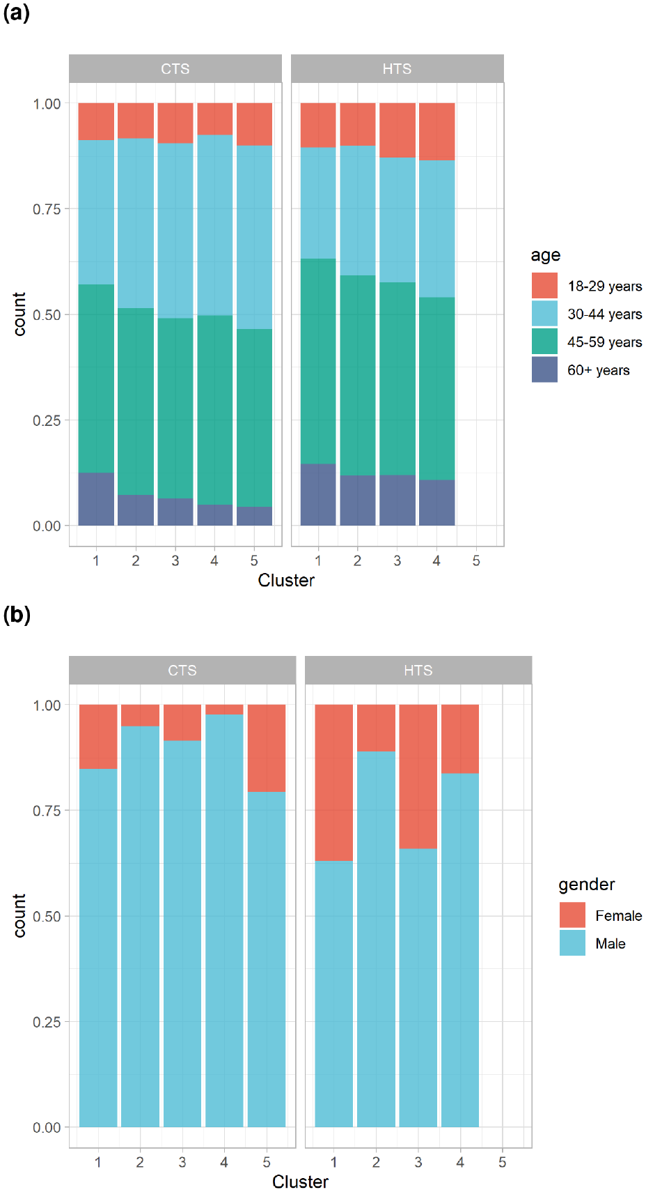
Figure 5 shows the relative distribution of the workers’ age in the top plot and their gender in the bottom plot. The age distribution is somewhat similar in both surveys and across clusters, indicating that both surveys represent the age of the working population with a slight shift toward older workers in the HTS.

Figure 5.

Scoiodeomographic characteristics of drivers by cluster and data source: (a) age of drivers and (b)gender of drivers.

Considering gender, we can identify a difference both between the surveys and across clusters. Looking at the two surveys, there are fewer female workers represented in the CTS compared with the HTS. This indicates that the CTS is less likely to include jobs that are more usually undertaken by women. Furthermore, there are also differences across the clusters. Female workers are more likely to be included in clusters 1 and 3 and less likely to be included in clusters 2 and 4. The latter include trip patterns that start rather early in the day. Such activities tend to be less compatible with child care obligations, which are still predominantly the woman’s responsibility in Germany.

Vehicle Characteristics

Figure 6 shows the characteristics of the vehicles. The top left plot shows vehicle age in the two surveys and across clusters, whereas the top right plot shows vehicle mileage. We can see that the vehicles reported in the CTS are in general newer than those reported in the HTS. This shows that the HTS captures primarily privately owned vehicles, whereas the CTS captures commercially owned vehicles because, in general, these have a shorter life cycle (i.e., for economic reasons). Nevertheless, differences between clusters are observable as well. Clusters 2 and 4 in the HTS and CTS include more vehicles less than 5 years old than the other clusters. These results are especially striking considering the mileage of these vehicles: over 60% of vehicles in the CTS have done over 100,000 km. This is in line with the definition of these clusters as representing long-distance travelers. The more a vehicle is used the shorter its life.

Figure 6.

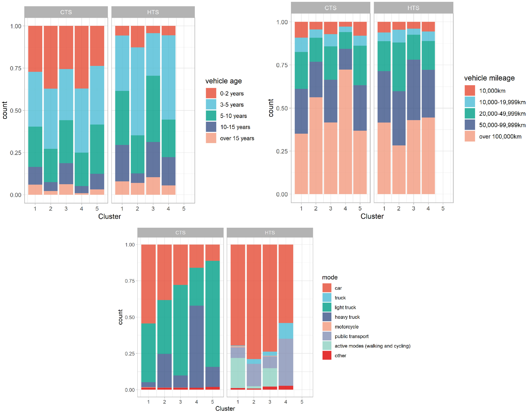
Vehicle characteristics: Vehicle age (top left), mileage (top right), vehicle type (bottom).

The comparison of vehicle types between the surveys proves to be more difficult because the CTS is a survey solely based on motorized vehicles, whereas the HTS covers all modes of transport. Nevertheless, we can still see some interesting effects. Workers in the CTS utilize trucks much more often than in the HTS, in which the car is the strictly dominant mode of transport. Furthermore, we can see that there is a general discrepancy between the surveys with regard to clusters 2 and 4: the large share of heavy trucks in the CTS indicates that these trips are undertaken for transportation purposes, but in the HTS a large share of the trips are undertaken by public transport, indicating that different trip and tour purposes are present with the same patterns. Additionally, because some truck trips are reported in the HTS but none at all in cluster 5, this shows that not only is there a systematic difference between the surveys but also that the response burden of reporting these trip patterns is too high to be included in the HTS. The evaluation of modes of transport reported in the HTS also indicates that a considerable proportion of work-related trips are undertaken using active modes of transport, indicating that work-related trips are not always undertaken with motorized vehicles.

Industry Sectors and Trip Purposes

Figure 7 shows the relative distribution of the vehicles and trips according to economic sector, industry sector, and purpose by cluster. The industry sectors are classified according to the Statistical Classification of Economic Activities in the European Community ( 51 ).

Figure 7.

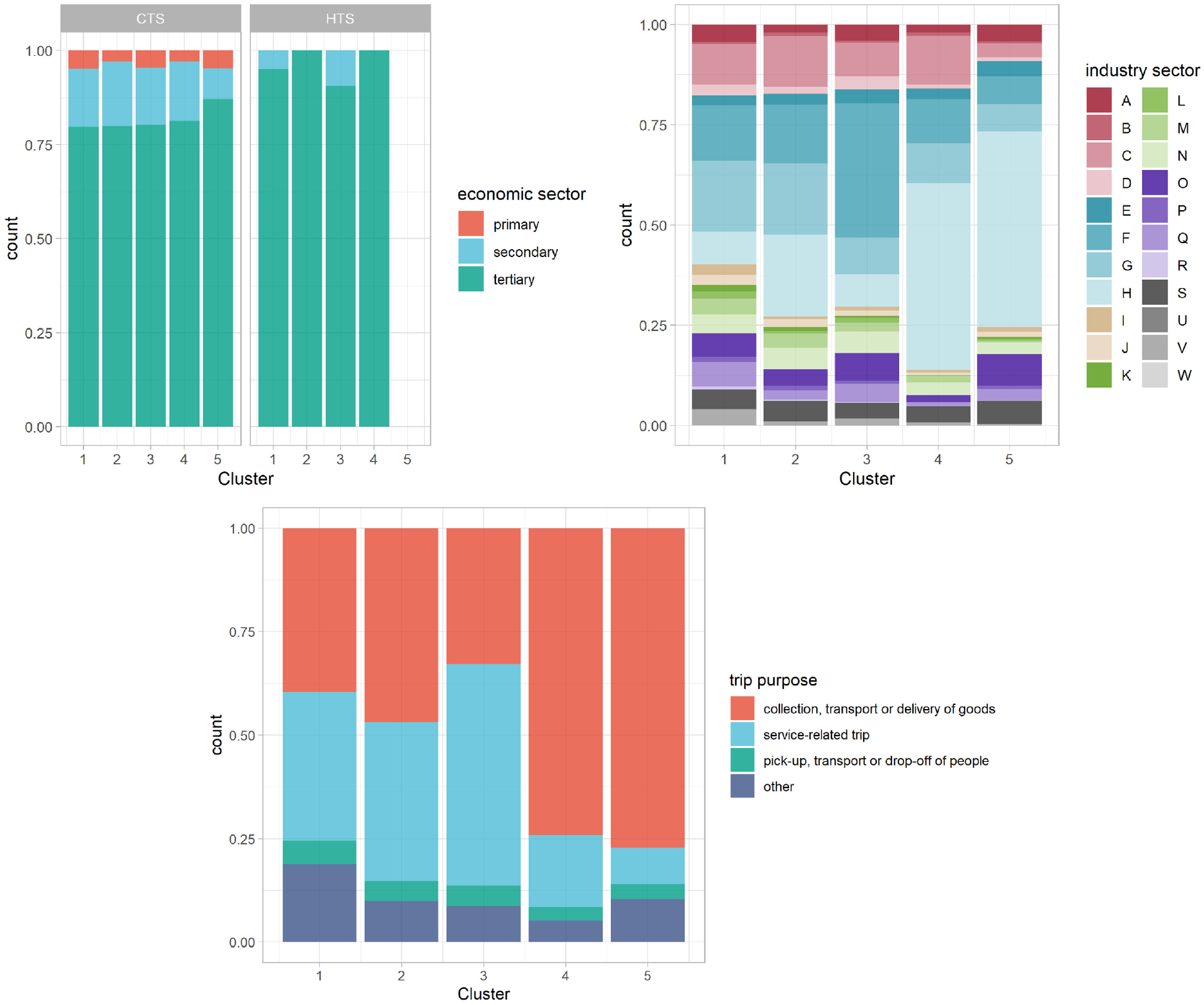
Relative distribution of vehicles and trips according to economic sector by data source (top left), industry sector (top right) and purpose (bottom) by cluster.

Considering the economic sector, we can see relevant differences across clusters and also across the two surveys. The share of vehicles belonging to the primary sector is relatively low as expected, because this sector includes industries that deal with raw products and are mostly fixed to single locations. This sector is not included in the HTS at all. The secondary sector includes manufacturing businesses. Although these industries are included in the HTS to some extent, the share is still relatively low. The most prevalent observations are attributed to the tertiary sector, also known as the service sector.

Clusters 1 and 2 show very similar distributions of both industry sector and trip purpose. This mostly holds true for the other categories as well, indicating that because the most striking difference is between the start time of the first trips, these clusters include workers from similar occupations who work during different parts of the day.

In cluster 3, the construction sector has the largest share. This is also supported by the distribution considering trip purpose in which the provision of a service makes up about 50%. The results indicate that this cluster mostly includes trip patterns of tradespeople who start their first trip somewhat early to go to the construction site. This is also consistent with the findings that this cluster includes fewer females and that the HTS presents with a large share of motorized vehicles and even some trucks. However, because a considerable share of trips are made using public transport, which is very unsuitable for tradespeople, we can assume there are also trip patterns that look like those of tradespeople but probably belong to workers with different occupations.

The industry sector most prevalent in clusters 4 and 5 is transportation. For these clusters, transportation of goods is the largest share with regard to trip purposes. These clusters are also those that include the fewest observations from the HTS, indicating that freight trips are generally not well represented here. Combining these findings with those pertaining to vehicle characteristics, the results indicate that clusters 4 and 5 include a lot of urban parcel deliveries; these would involve high mileage, but the trips would be undertaken using light trucks.

Implications and Limitations of the Study

There are several overarching implications of our study for survey designers, transport planners, and policymakers. Our results show that work-related travel patterns are quite complex and diverse. Although there are some patterns that are well represented in both the HTS and CTS, trips undertaken by highly mobile workers in particular are not present in the HTS. These results are consistent with findings in previous studies on underrepresentation of trips in HTSs ( 1 , 2 ). Our results supplement these findings by identifying that workers from the transportation sector in particular are either not included in the sample from the HTS or underreport their trips. These results suggest that the HTS should include more work-related variables to assess which work-related trips are covered by the surveys and identify those workers for whom the survey is not sufficient. We suggest that this should be recognized in future HTSs because currently they gather little information neither on work-related trips nor industry- and occupation-specific variables, which are an important factor in the generation of commercial trips (22 –24). Including more information on the occupational status of the survey participants would also help in the study of other work-related effects on transport such as teleworking. Previous studies have shown that teleworking influences travel behavior and can help reduce peak-hour traffic and the number of other work-related trips; however, not everybody can work from home, primarily because of the nature of their work ( 16 , 17 ). To quantify these effects, more information on survey participants’ working conditions is needed.

Our analyses further show that the travel patterns are formed according to different jobs and with different vehicles. Although this and other establishment-based (27 –29) surveys provide much more detailed information on companies, they only cover trips undertaken by motorized vehicles. However, our results show that not all work-related trips are undertaken with motorized vehicles. For example, although technical occupations (tradespeople) are well covered in the CTS, other occupations showing similar work-related trip patterns, especially those using other modes of transport, are not considered adequately.

Although we found that some travel patterns are not represented in the HTS at all, our findings show there is a considerable overlap between the HTS and the CTS. This indicates that the surveys do not fully complement each other but that they gather redundant data. When used for forecasting and travel demand modeling, this may lead to biased results if not handled correctly because superposition of trips from both surveys may not provide the true work-related travel demand. This also needs to be considered in the evaluation of policy measures. Car-free policies often only consider private cars and specifically exclude commercial vehicles ( 52 ); however, because work-related transport is often not modeled adequately, the full effect is difficult to forecast. This also holds true for policies that promote the transition to electric vehicles. Gnann et al. ( 53 ) studied the market potential of plug-in electric vehicles in Germany. However, as our results show, the effects are hard to quantify because of the ambiguous data sources.

There are also some limitations of this study worth noting. Hilsop ( 21 ) finds that the work-related travel patterns of nonmanagerial workers are often overlooked in studies. Because the CTS does not contain information on the occupational status of the workers either, this cannot be assessed by our study. We suggest that future CTSs should also include more detailed sociodemographic information. This is also highlighted by Mohino et al. ( 18 ), who find that sociodemographic information significantly influences work-related travel patterns.

The work presented here is specific to Germany, because data sources allowed for a comprehensive analysis. Although we may expect similar effects in other countries, further research is needed to confirm this assumption. Furthermore, the data sources are both relatively old and the findings need to be validated against newer data. This is especially important considering that work-related transport is strongly correlated to commercial activity and the economic situation, both of which can be very dynamic. However, although HTSs are conducted regularly this is not the case for CTSs.

This study is intended as an exploratory analysis of work-related trip patterns and should be regarded as the first step toward improving knowledge about commercial transport and required data sources. Although the variables used are generally consistent across the two surveys in the cluster analysis, we recognize that in the future, the data used in this study should be supplemented by other sources to improve the ratio between CTS and HTS observations.

Future work will include analysis based on other data sources such as sensor data in urban areas and GPS tracking from vehicles to assess whether these passive data sources could supplement HTSs, which are known to have a high response burden. Furthermore, it should be examined whether and how different economic situations influence work-related mobility and whether this can be seen in the surveys.

Conclusion

This study examines work-related trip patterns in traditional HTSs and CTSs. It is intended to increase insights into work-related travel patterns and their representation in the respective surveys.

The results shows that work-related travel patterns are quite complex. Although some patterns are covered in both the HTS and CTS, the travel patterns of mobile workers from the transportation sector in particular are not well represented in the HTS. Contrary to this is the problem that the CTS usually only surveys trips undertaken by motorized vehicles. However, our analysis shows that a considerable share of work-related trips are undertaken using public transport or active modes of transport. This is an important factor when assessing policy measures. Our results indicate that some work-related trip patterns involve nonmotorized transport, and policies focusing on commercial transport should not only target vehicle types but also modal shifts.

The results indicate that researchers and transport planners creating travel demand models need to pay more attention to work-related travel behavior and acknowledge that depending on the area of study, although traditional HTSs may not provide a complete sample of the population, simply adding data on commercial trips from commercial travel demand models to data from HTSs does not provide a complete picture of work-related travel either. The design of separate surveys in itself is not problematic, but they should include variables that can be used to identify which work-related trip patterns are included in which survey and whether supplemental data sources are needed.

Footnotes

Acknowledgements

We would like to thank the five anonymous referees who reviewed this paper for providing helpful suggestions and comments to improve the manuscript.

Author Contributions

The authors confirm contribution to the paper as follows: study conception and design: A. Reiffer, L. Barthelmes, M. Kagerbauer, P. Vortisch; data collection: A. Reiffer; analysis and interpretation of results: A. Reiffer, L. Barthelmes; draft manuscript preparation: A. Reiffer, L. Barthelmes. All authors reviewed the results and approved the final version of the manuscript.

Declaration of Conflicting Interests

The author(s) declared no potential conflicts of interest with respect to the research, authorship, and/or publication of this article: We acknowledge support by the KIT-Publication Fund of the Karlsruhe Institute of Technology.

Funding

The author(s) disclosed receipt of the following financial support for the research, authorship, and/or publication of this article:

ORCID iDs

Anna Reiffer

Lukas Barthelmes

Martin Kagerbauer

Peter Vortisch

Data Accessibility Statement

The data sets used in this research are available from the Traffic Clearinghouse at the German Aerospace Center (DLR).

References

Brög

Winter

Untersuchungen zum Problem der non-reported-trips zum Personen-Wirtschaftsverkehr bei Haushaltsbefragungen. Forschung Straßenbau und Straßenverkehrstechnik, No. 593, 1990.

Itsubo

Hato

Effectiveness of Household Travel Survey Using GPS-Equipped Cell Phones and Web Diary: Comparative Study with Paper-Based Travel Survey. Presented at 85th Annual Meeting of the Transportation Research Board, Washington, D.C., 2006.

Stopher

FitzGerald

Assessing the Accuracy of the Sydney Household Travel Survey with GPS. Transportation, Vol. 34, No. 6, 2007, pp. 723–741. https://doi.org/10.1007/s11116-007-9126-8.

Evans

Cummings

Slocombe

Corvaglia

National Travel Survey: England 2017. Department for Transport, London, 2018.

KiM Netherlands Institute for Transport Policy Analysis. Mobility Report 2016. KiM Netherlands Institute for Transport Policy Analysis, The Hague, 2016.

Nobis

Kuhnimhof

Mobilität in Deutschland. Federal Ministry of Transport and Digital Infrastructure, Bonn, 2019.

Transport for London. Travel in London. Report 11. Transport for London, London, 2018.

Nilles

Carlson

Gray

Hanneman

Telecommuting – An Alternative to Urban Transportation Congestion. IEEE Transactions on Systems, Man, and Cybernetics, Vol. 6, No. 2, 1976, pp. 77–84.

Hamer

Kroes

van Ooststroom

Teleworking in the Netherlands: An Evaluation of Changes in Travel Behaviour. Transportation, Vol. 18, No. 4, 1991, pp. 365–382.

10.

Henderson

D. K.

Koenig

B. E.

Mokhtarian

P. L.

Using Travel Diary Data to Estimate the Emissions Impacts of Transportation Strategies: The Puget Sound Telecommuting Demonstration Project. Journal of the Air & Waste Management Association, Vol. 46, No. 1, 1996, pp. 47–57. https://doi.org/10.1080/10473289.1996.10467440.

11.

Kitamura

Nilles

Conroy

Fleming

Telecommuting as a Transportation Planning Measure: Initial Results of California Pilot Project. Transportation Research Record: Journal of the Transportation Research Board, 1990. 1285: 98–104.

12.

Pendyala

Goulias

Kitamura

Impact of Telecommuting on Spatial and Temporal Patterns of Household Travel. Transportation, Vol. 18, No. 4, 1991, pp. 383–409. https://doi.org/10.1007/BF00186566.

13.

Rhee

H.-J.

Home-Based Telecommuting and Commuting Behavior. Journal of Urban Economics, Vol. 63, No. 1, 2008, pp. 198–216. https://doi.org/10.1016/j.jue.2007.01.007.

14.

Lachapelle

Tanguay

G. A.

Neumark-Gaudet

Telecommuting and Sustainable Travel: Reduction of Overall Travel Time, Increases in Non-Motorised Travel and Congestion Relief?

Urban Studies, Vol. 55, No. 10, 2018, pp. 2226–2244. https://doi.org/10.1177/0042098017708985.

15.

Caulﬁeld

Does It Pay to Work from Home? Examining the Factors Inﬂuencing Working from Home in the Greater Dublin Area. Case Studies on Transport Policy, Vol. 3, No. 2, 2015, pp. 206–214. https://doi.org/10.1016/j.cstp.2015.04.004.

16.

Mokhtarian

P. L.

Salomon

Modeling the Choice of Telecommuting: 2. A Case of the Preferred Impossible Alternative. Environment and Planning, Vol. 28, 1996, pp. 1859–1876.

17.

Mokhtarian

P. L.

Salomon

Modelling the Choice of Telecommuting: 3. Identifying the Choice Set and Estimating Binary Models for Technology-Based Alternatives. Environment and Planning, Vol. 28, 1996, pp. 1877–1894.

18.

Mohino

Solis

Urena

J. M.

The Inﬂuence of Education Level and Job Type on Work-Related Travel Patterns within Rural Metro-Adjacent Regions. Journal of Transport and Land Use, Vol. 12, No. 1, 2019, pp. 73–98.

19.

Beaverstock

J. V.

Budd

International Business Travel in a Digital World Economy. Research in Transportation Business & Management, Vol. 9, 2013, pp. 1–4. https://doi.org/10.1016/j.rtbm.2013.09.001.

20.

Jeong

Y.-J.

Zvonkovic

A. M.

Sano

Acock

A. C.

The Occurrence and Frequency of Overnight Job Travel in the USA. Work, Employment and Society, Vol. 27, No. 1, 2013, pp. 138–152.

21.

Hislop

The Diverse Patterns of Work-Related Business Travel: Accounting for Spatial Scale. Applied Mobilities, Vol. 1, No. 2, 2016, pp. 219–233.

22.

Steinmeyer

Wagner

Using National Behavioral Data on Commercial Trafﬁc for Local and Regional Applications. Presented at 85th Annual Meeting of the Transportation Research Board, Washington, D.C., 2006.

23.

Hebes

Menge

Lenz

Service Trafﬁc: An Entrepreneurial View on Travel Behaviour. Proc., 12th World Conference on Transport Research, Lisbon, Portugal, 2010.

24.

Aguilera

Business Travel and Mobile Workers. Transportation Research Part A: Policy and Practice, Vol. 42, No. 8, 2008, pp. 1109–1116.

25.

Allen

Anderson

Browne

Wigan

Understanding the Growth in Service Trips and Developing Transport Modelling Approaches to Commercial, Service and Light Goods Movements. Association for European Transport, London, 2002.

26.

Menge

Hebes

Intermodal Service Trafﬁc – State of the Practice or Scientiﬁc Demand?

Studies on Mobility and Transport Research, Vol. 1, 2008, pp. 53–70.

27.

Hunt

Stefan

Brownlee

Establishment-Based Survey of Urban Commercial Vehicle Movements in Alberta, Canada: Survey Design, Implementation, and Results. Transportation Research Record: Journal of the Transportation Research Board, 2006. 1957: 75–83.

28.

Steinmeyer

Kenndaten der Verkehrsentstehung im Personenwirtschaftsverkehr: Analyse der voranschreitenden Ausdifferenzierung von Mobilitätsmustern in der Dienstleistungsgesellschaft. Hamburg University of Technology Reports on Transport Planning and Logistics, Vol. 3. Huss-Verlag, München, 2004.

29.

Wermuth

Neef

Wirth

Hanitz

Löhner

Hautzinger

Mobilitätsstudie Kraftfahrzeugverkehr in Deutschland 2010 (KiD 2010). Final report. Verkehrsforschung und Infrastrukturplanung, Baunschweig, 2012.

30.

Stefan

McMillan

Hunt

Urban Commercial Vehicle Movement Model for Calgary, Alberta, Canada. Transportation Research Record: Journal of the Transportation Research Board, 2005. Vol. 1921: 1–10.

31.

Hunt

J. D.

Stefan

K. J.

Tour-Based Microsimulation of Urban Commercial Movements. Transportation Research Part B: Methodological, Vol. 41, No. 9, 2007, pp. 981–1013. https://doi.org/10.1016/j.trb.2007.04.009.

32.

Gliebe

Cohen

Hunt

J. D.

Dynamic Choice Model of Urban Commercial Activity Patterns of Vehicles and People. Transportation Research Record: Journal of the Transportation Research Board, 2007. 2003: 17–26.

33.

Ferguson

Maoh

Ryan

Kanaroglou

Rashidi

T. H.

Transferability and Enhancement of a Microsimulation Model for Estimating Urban Commercial Vehicle Movements. Journal of Transport Geography, Vol. 24, 2012, pp. 358–369. https://doi.org/10.1016/j.jtrangeo.2012.04.013.

34.

Ellison

R. B.

Teye

Hensher

D. A.

Modelling Sydney’s Light Commercial Service Vehicles. Transportation Research Part A: Policy and Practice, Vol. 96, 2017, pp. 79–89.

35.

Reiffer

Heilig

Kagerbauer

Vortisch

Microscopic Demand Modeling of Urban and Regional Commercial Transport. Procedia Computer Science, Vol. 130, 2018, pp. 667–674. https://doi.org/10.1016/j.procs.2018.04.118.

36.

Reiffer

Heilig

Szimba

Klenner

Kagerbauer

Vortisch

Combining Macro- and Microscopic Approaches to Model Commercial Transport Demand in an Urban Area. Transportation Research Procedia, Vol. 48, 2020, pp. 574–589.

37.

Primerano

Taylor

M. A.

Pitaksringkarn

Tisato

Deﬁning and Understanding Trip Chaining Behaviour. Transportation, Vol. 35, No. 1, 2008, pp. 55–72.

38.

Institute for Applied Social Sciences and German Aerospace Center. Mobilität in Deutschland 2008. Infas, Bonn, 2010.

39.

Webb

A. R.

Cawley

Copsey

K. D.

Statistical Pattern Recognition, 3rd ed. Wiley-Blackwell, Oxford, 2011. https://doi.org/10.1002/9781119952954.

40.

Adolfsson

Ackerman

Brownstein

N. C.

To Cluster, or Not to Cluster: An Analysis of Clusterability Methods. Pattern Recognition, Vol. 88, 2019, pp. 13–26.

41.

Hartigan

J. A.

Hartigan

P. M.

The Dip Test of Unimodality. The Annals of Statistics, Vol. 13, No. 1, 1985, pp. 70–84.

42.

Silverman

B. W.

Using Kernel Density Estimates to Investigate Multimodality. Journal of the Royal Statistical Society: Series B (Methodological), Vol. 43, No. 1, 1981, pp. 97–99.

43.

Ahmed

M. O.

Walther

Investigating the Multimodality of Multivariate Data with Principal Curves. Computational Statistics & Data Analysis, Vol. 56, No. 12, 2012, pp. 4462–4469.

44.

Aggarwal

C. C.

Reddy

C. K.

Data Clustering: Algorithms and Applications. Chapman & Hall/CRC Press, London, 2014.

45.

R Core Team. R: A Language and Environment for Statistical Computing. 2019. https://www.R-project.org/. Accessed July 31, 2021.

46.

Murtagh

Legendre

Ward’s Hierarchical Agglomerative Clustering Method: Which Algorithms Implement Ward’s Criterion?

Journal of Classiﬁcation, Vol. 31, No. 3, 2014, pp. 274–295. https://doi.org/10.1007/s00357-014-9161-z.

47.

Thorndike

R. L.

Who Belongs in the Family?

Psychometrika, Vol. 18, No. 4, 1953, pp. 267–276. https://doi.org/10.1007/BF02289263.

48.

Xiong

Clustering Validation Measures. In Data Clustering ( Aggarwal

C. C.

Reddy

C. K.

, eds.), Chapman and Hall/CRC Press, London, 2018, pp. 571–606.

49.

Liu

Xiong

Gao

Understanding and Enhancement of Internal Clustering Validation Measures. IEEE Transactions on Cybernetics, Vol. 43, No. 3, 2013, pp. 982–994.

50.

Van Buuren

Groothuis-Oudshoorn

MICE: Multivariate Imputation by Chained Equations in R. Journal of Statistical Software, Vol. 45, No. 1, 2011, pp. 1–67.

51.

Ec.europa.eu. 2022. Statistical Classification of Economic Activities in the European Community, Rev. 2 (2008). Accessed April 19, 2022.

52.

Nieuwenhuijsen

M. J.

Khreis

Car Free Cities: Pathway to Healthy Urban Living. Environment International, Vol. 94, 2016, pp. 251–262.

53.

Gnann

Plöz

Funke

Wietschel

What is The Market Potential of Plug-In Electric Vehicles as Commercial Passenger Cars? A Case Study from Germany. Transportation Research Part D: Transport and Environment, Vol. 37, 2015, pp. 171–187.

Representation of Work-Related Trip Patterns in Household and Commercial Travel Surveys

Abstract

Keywords

Materials and Methods

Data

Data Preparation

Descriptive Analysis

Cluster Analysis

Results and Discussion

Cluster Characteristics

Activity Duration

Sociodemographic Characteristics of Workers

Vehicle Characteristics

Industry Sectors and Trip Purposes

Implications and Limitations of the Study

Conclusion

Footnotes

Acknowledgements

Author Contributions

Declaration of Conflicting Interests

Funding

ORCID iDs

Data Accessibility Statement

References