
Abstract
This paper investigates the changes caused by the COVID-19 pandemic on households’ perceived utility of the accessibility of their residence in the Greater Toronto and Hamilton Area (GTHA). The paper considers several neighborhood and dwelling attributes and fuses those with property price data from mid-March 2019 to mid-March 2021 to analyze changes in housing trends before and during the COVID-19 pandemic. Two mixed geographically weighted regression (MGWR) models are estimated for the year before the start of the pandemic and the year during the pandemic to address spatial autocorrelation and non-stationarity in price data. The empirical models reveal new patterns in accessibility perception for some factors, including accessibility to regional subway and inter-regional rail transit. This study also contributes to the literature of MGWR modeling by assessing the capacity of the model through validation procedures. Estimation is performed on randomly selected samples from the population to compare the errors with the population-based model and a traditional hedonic price model. The findings suggest that the application of MGWR is restricted to cases where price data are abundant.
Since the novel
The literature identifies four aspects in accessibility measurements: (1) the land-use component, (2) the transportation component, (3) the temporal component, and (4) the individual component ( 8 ). Each of these components is subject to alterations resulting from the pandemic experience. For instance, the disutility of transit trips from an origin to a destination could have changed for individuals during the pandemic because of higher infection risks and consequently changed their perception of the transport component of the accessibility of their residence for different modes. Also, during the COVID-19 pandemic, households have been exposed to new daily routines where their former work and non-work activities were replaced by Information Communication Technologies (ICT) such as telecommuting, distance learning, and online shopping. This exposure by releasing the temporal constraint could disrupt the temporal component of the availability of work and recreational activities. From individual perspectives, there is also the possibility of households’ loss of income through unemployment or even death of a member, which could modify households’ perception of their residence accessibility.
The importance of studying households’ perception of the accessibility of their residence stems from the hierarchical nature of travel choices, where households’ current long-term choices will eventually affect their future short-term travel choices ( 9 ). If a household, because of changes to its perceived accessibility, no longer considers its current residence accessible to activities, it will enter the market and relocate its residence. On a larger scale, the combination of relocation patterns will dictate future travel behaviours and investments. So far, COVID-19 vaccination effects have been promising in controlling the spread of the virus. The closer we get to the end of the pandemic, the more we should shift our focus from immediate adjustments of travel behaviour to the long-lasting effects of the pandemic on travel behaviour. It is important to mention that capturing the overall long-term impacts of the COVID-19 pandemic requires ongoing investigation of households’ behaviour changes in the coming years until the behavioural changes stabilize. This study explores how pandemic lifestyle changes have adjusted the households’ perception of accessibility in the Greater Toronto and Hamilton Area (GTHA) during the first year of the pandemic. This study examines whether households’ preferences for proximity to certain points of interest have changed through the first year of the COVID-19 pandemic.
This study analyzes the entire GTHA residential property transactions for a year before and after the provincial government’s lockdown announcement in mid-March 2020 ( 10 ). The basis of our study is the hypothesis that property transaction price represents the compensation to the buyer’s perceived utility and the utilities they gain by various dwelling amenities. In the transportation field this is a common hypothesis, and it has been mainly implemented to combine utilities of transportation demand models with location choice and price models. For instance, UrbanSim, which is a Land Use and Transportation Integrated (LUTI) framework, treats land price as a disutility in the location choice model ( 11 ), and TRANUS, another LUTI framework, combines it with travel costs to represent the trade-off between transportation costs and property rent costs at the macro-level ( 12 ).
In this paper, we argue that the price buyers pay for a property is the compensation for the perceived utility, and it can be divided into two main components: (1) the utility the buyer gets from the attributes related to the dwelling’s overall quality and characteristics, such as the property’s floor area and the number of bedrooms, and (2) the utility of the property’s location by the accessibility it provides to the buyer’s daily activities. Property buyers are making a trade-off between enhancing their dwelling characteristics versus increasing their accessibility (i.e., reducing mobility costs) when allocating their budget for purchasing a property. This budget-constrained trade-off is the foundation of our analysis in this paper. We later compare the changes in the significance of accessibility-related variables a year before and after the lockdown.
From the methodological perspective, our analyses for this study are founded on the following elements:
This study uses the mixed geographically weighted regression (MGWR) for modeling property transaction prices to address the spatial effects in the dataset.
Isochrones-based accessibility measurements are implemented to examine the influence of accessibility factors in the price model.
In the model estimation process, first, we train a reference price model using a subset of all transactions. Then, we investigate the importance of considering spatial effects by estimating a set of methodologically simpler models.
By having access to the whole population of transactions, this paper also adds to the literature by testing the performance of the MGWR model in different sample sizes. We apply the MGWR model to random population samples to see how its goodness of fit is related to the sample size. Fotheringham et al. state that as the sample size decreases, weighted regression’s ability to capture spatial effects decreases, but the evidence in the literature is sparse ( 13 ). To explore this property, we take advantage of our access to population data and examine variation between the prediction errors of equal-sized random samples and the reference model for estimated MGWR and hedonic price models.
The remainder of the paper is structured as follows. The next section reviews the literature to highlight the contributions of this study, and after this the concepts of the MGWR model and the estimation procedure are introduced. Input data are then discussed, followed by a section presenting model results. The final section provides conclusions and recommendations for further research.
Literature Review
Residential Property Price Models
In early studies, researchers divided the study area into multiple regions and compared statistical measures to track changes over time and space. Gatzlaff and Smith for Miami compare residential prices over time ( 14 ), and Armstrong and Robert for Boston compare residential prices over space for areas with transit-oriented development ( 15 ). Although these studies manage to capture the positive relationship between transit development and residential property prices, they are based on finding patterns of growth rather than causal relationships. As such, they cannot give reliable inferences in relation to the magnitude of future transportation development and property value uplift.
Another popular approach uses cross-sectional data to create a hedonic price model, as originally proposed by Rosen ( 16 ), to investigate the significant variables in the price of residential properties. Hedonic price models generate an estimate of space price expressed as a function of a set of independent variables describing characteristics of the dwelling, its environment, and its accessibility to amenities. Two early applications are by Landis et al. for California ( 17 ) and Chen et al. for Portland ( 18 ).
According to Miron, although hedonic price models investigate the role of a wide range of factors affecting residential property prices, they overlook the possible existence of spatial autocorrelation and spatial non-stationarity within the dataset ( 19 ). Results and conclusions may be unreliable for price estimation and policy analysis. Therefore, modeling the relationship between property price uplift and transportation network improvement solves spatial non-stationarity in these global models.
Kim and Kim apply spatial lag models (SLMs) and spatial autoregressive error models (SEMs) to residential price determination and conclude that the SEM better captures spatial dependencies and produces a stronger model for price estimation ( 20 ). Spatial Durbin models (SDMs) are another modification to deal with spatial effects. In the literature of transportation and residential price, SDM is used by Efthymiou and Antoniou for Athens ( 21 ) and Hawkins and Habib for the Greater Toronto Area ( 22 ). Osland argues that SDMs are useful when modeling time-series data and can be developed from either SLMs or SEMs ( 23 ). Finally, Fotheringham et al. propose geographically weighted regression (GWR) based on moving window regression ( 13 ). Du and Mulley implement a GWR model to develop a model of residential property prices for London, UK ( 24 ).
Property Prices and Transportation Accessibility
Table 1 summarizes the studies conducted to investigate the relationship between proximity to the transportation network and residential property prices by focusing on methods, sample size, and critical findings related to the objective of our study. The primary objective of most of the studies mentioned in Table 1 is to investigate how different transportation developments affected the residential property prices in their proximity. This paper takes a different approach to explore the changes in the magnitude of accessibility-related attributes before and during the COVID-19 pandemic caused by households’ pandemic experience as no significant transportation development happened in the GTHA. Nonetheless, a review of these studies assists the reader in seeing the way transportation accessibility variables are implemented in residential property price models.
Summary of Literature Review on the Relationship Between Transportation Development and Residential Property Prices/Rents
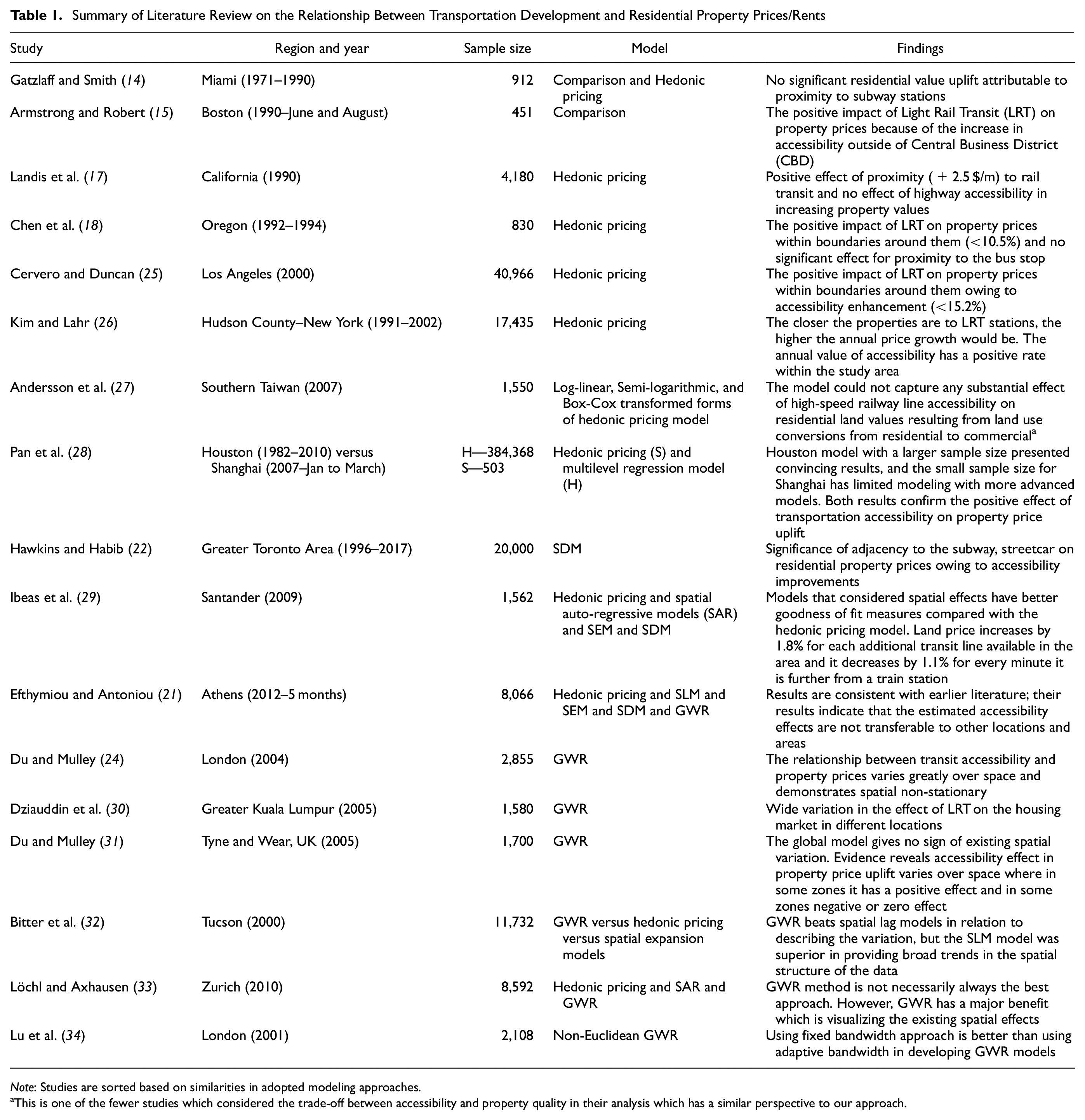
Note: Studies are sorted based on similarities in adopted modeling approaches.
This is one of the fewer studies which considered the trade-off between accessibility and property quality in their analysis which has a similar perspective to our approach.
In summary, several methodologies have been implemented in the literature to address the spatial effects in the dataset. The current study identifies the GWR method as the best fit for the purpose of this study for two main reasons. First, unlike other methods, the GWR model provides the spatial distribution of parameter estimations by the definition of local variables, which provides deeper spatial information on accessibility perception changes ( 35 ). Second, looking at studies that implement GWR and because GWR is based on moving regression windows, it is suggested that GWR performs better if applied to many data points ( 24 ). Yet, because Löchl and Axhausen reported that residuals in the GWR model for residential rents can still be correlated ( 33 ), we also control for spatial autocorrelation in residuals in the GWR model for residential land prices to test whether GWR has successfully captured the spatial effects in our dataset. The next section introduces the GWR and mixed GWR models (the version of the model used in this study).
Methods of Analysis
Global and Local Regressions
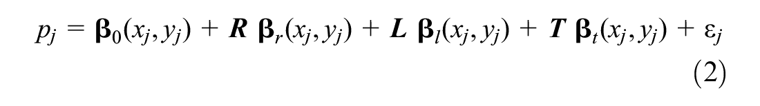
GWR is a modification of a hedonic pricing model with two primary objectives: (1) solving the spatial non-stationarity problem in global regression models and (2) creating a continuous model structure rather than having several local regressions. The starting point is also a global regression model with property price as a function of real estate characteristics and transportation-related variables

where
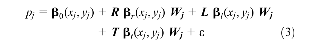
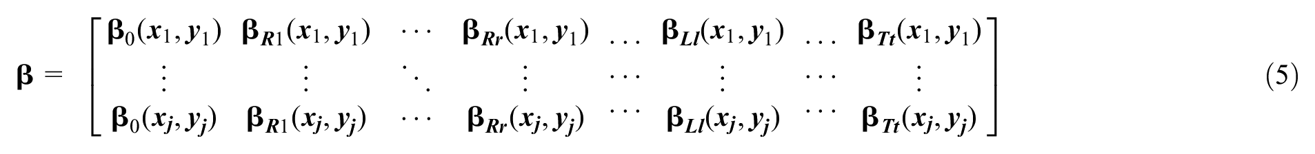
To address the autocorrelation issue and deal with spatial non-stationarity associated with assuming global parameters, GWR extends the global model to consider local regressions points individually. Thus, instead of having one coefficient for each independent variable, the model will produce a surface of coefficients according to the following equation.
where each j is a regression point, and the set of regression points can be a subset of i.
where
Now consider
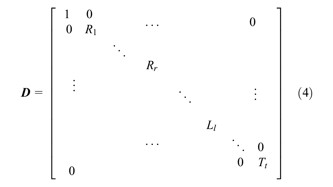
Therefore, considering

Accordingly, a weighted least squares method can be used to estimate the parameters. Equation 7 shows a single row of the

Mixed Geographically Weighted Regression
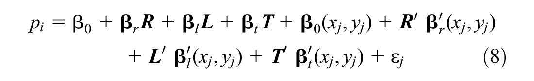
In relation to computation cost, it is more efficient if the model keeps independent variables global if they do not exhibit spatial variation. This is the objective of MGWR, which is a mixture of the global regression model and the original GWR model. The formulation of the MGWR model is demonstrated in Equation 8,
As it is unknown whether a variable should be modeled as global or local, this study uses a trial-and-error method to gain the best possible fit for the data. At the start, every variable is treated as global, and the model makes one variable from the global regression a local variable. If this change produces a better model—a lower Akaike Information Criterion (AIC)—the model keeps the change. Otherwise, it continues the procedure on the original model. After a variable is made local, the model reverses the process and switches variables from the local model to the global model, keeping changes if the AIC improves. The explained criterion for comparing model goodness of fit when a variable is defined as local or global was originally proposed by Nakaya et al. ( 36 ). The procedure continues until it has added and dropped every variable and found the best combination.
Another important decision for the model structure is choosing the weighting structure between regression points and observations. This study uses an adaptive Gaussian kernel type, which is the most flexible method. Adaptive kernels choose the optimum kernel for each regression window based on minimizing the AIC ( 13 ). Moreover, it is shown by Bidanset and Lombard that the Gaussian kernel weights the observations better than its rival bi-square kernel in the context of real estate modeling, and it produces a model with better goodness of fit ( 37 ).
We consider two aspects of the MGWR model: (1) the effect of sample size on the variation of individual parameters and (2) the predictive ability of the MGWR model. In the first instance, most studies do not have access to population data and follow the assumption of the Law of Large Numbers that sample results are representative of the population. In a traditional linear model, increasing the sample size will asymptotically reduce parameters’ standard errors. However, additional observations raise the number of regression points (individual effect models) with GWR, and the model does not necessarily obey asymptotic properties. In the second instance, GWR is usually applied to descriptive analysis in the literature. Given our access to the full population, we can estimate the model with a random sample and validate the model with several random samples.
Data Preparation Process
Real Estate Data Collection
The timeline of our dataset is from March 17, 2019, to March 16, 2020 (one year before Ontario entered the state of emergency) and March 17, 2020, to March 16, 2021 (a year during the COVID-19 pandemic). For 298 days through the first year of the pandemic, more than any other major city in the world ( 38 ), Toronto has been in various stages of the lockdown phase. For both time periods, this article uses combined real estate data from the Toronto Regional Real Estate Board (TRREB) and Information Technology Systems Ontario (ITSO) to acquire all transactions in the GTHA. After excluding incomplete entries, the sample size for the year before the pandemic the first year during the pandemic consists of 93,966 and 96,513 records, respectively. To the best of our knowledge, this is among the first studies to model disaggregate residential property prices at the population level. Variables included in the dataset are real estate-related variables, including; dwelling types, house area, construction type, front exposure, number of bedrooms, washrooms, parking spots, and maintenance fees and property tax.
Adding Transportation Accessibility Measurements Using Enhanced Points of Interest
We have used two other data sources to add the accessibility measurements to the property price dataset: (1) Open-source General Transit Feed Specification (GTFS) to identify a property’s access to public transit, and (2) enhanced points of interest from DMTI Spatial Inc. for 2019 ( 39 ) to acquire amenities around the residential properties. Then, using Geographical Information System processing, the isochrones-based accessibility measures are computed to count the number of opportunities within certain distances of each sold property. It is worth acknowledging that isochrones-based accessibility measures are one of the simpler methods for accessibility measurements ( 40 ). However, this is the limitation inherent in the nature of this study as land price data lack information on the household who purchase the property, which restricts the use of more complicated attraction-based and utility-based measurements.
Variables added to the dataset in this step can be defined in two categories. The number of amenities within a quarter quarter-mile of properties is added to the dataset in the first category. The number of grocery shops, retail stores, eating and drinking places, drugstores, medical clinics, and educational institutions are added in this category. It is worth mentioning that the dataset does not include information on the level of attractiveness of different amenities, and in our study we put the same weight on all amenities in each category. In the second category, the number of subway stations within a half-mile distance and the number of bus stops in quarter miles are added to the dataset. The second category comprises variables that are related to transportation and transit attributes. Lastly, as the TRREB real estate database uses imperial units, all distances are set in miles.
Results and Discussion
In GWR, the number of regression points can increase to the number of observations, and therefore, the computation cost can be high. Using MGWR further increases this computation cost as it introduces the global-to-local and local-to-global variable searches. To deal with this massive computation cost, we divide the estimation process into three steps. The process of MGWR estimation is summarized in Figure 1 and detailed in the subsequent subsections.
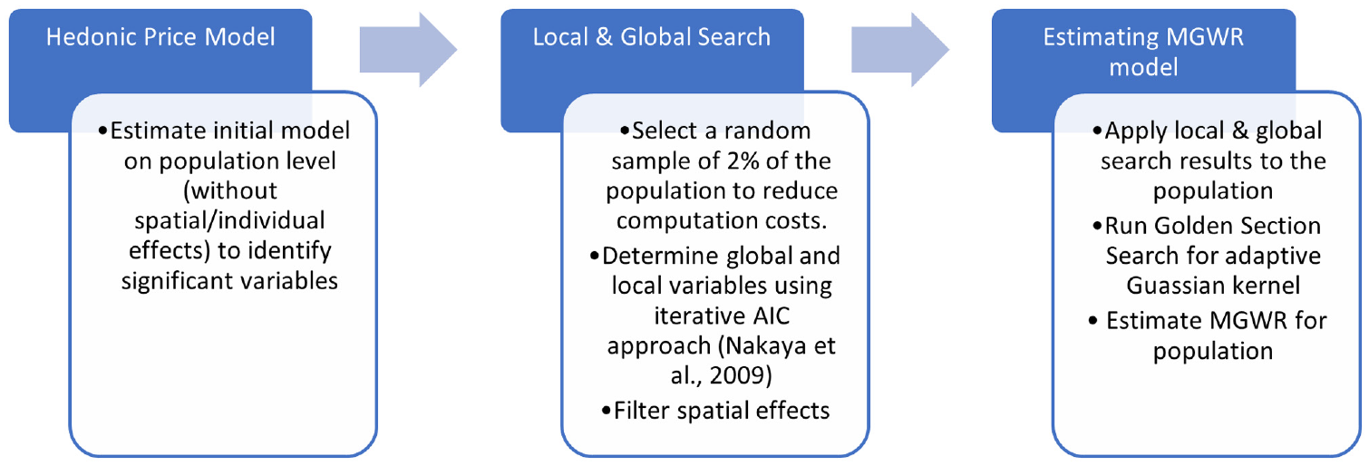
Estimation process.
Global Regression Results
The model estimation starts with a global regression model. This starting point helps the MGWR model in two ways. First, it produces a conventional hedonic pricing model, which can be useful in providing a bigger picture in relation to variable selections. Through this practice, we identify the significant variables and include them in the Local and Global search algorithm. Second, the hedonic price model can be a reference for testing the spatial heterogeneity in the GWR model. The results of the global model are presented in Table 2. We note that some insignificant variables in the hedonic price model may become significant at the local level when applied in the GWR model. However, carrying the variable selection process through to the final model has a high time cost. Also, our objective is to compare models with a hedonic price model with significant parameters, which would be included in a model used for prediction.
Global Regression Results a (Hedonic Price Models)
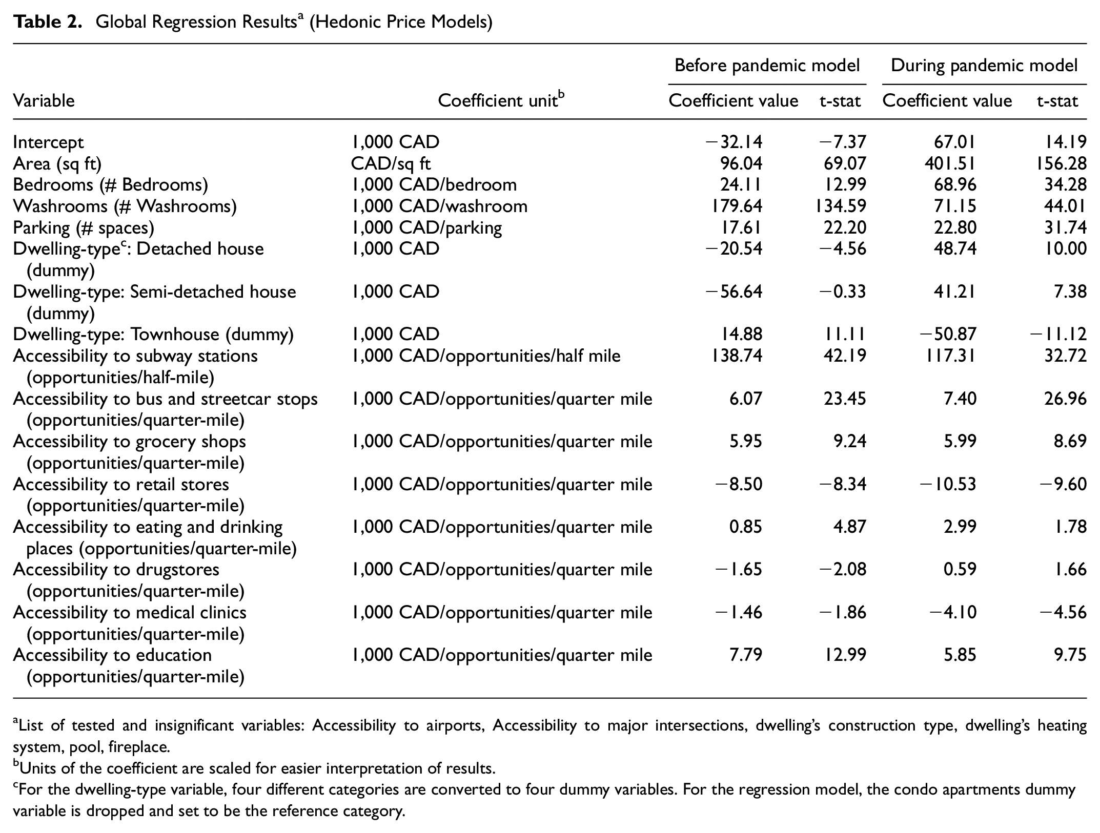
List of tested and insignificant variables: Accessibility to airports, Accessibility to major intersections, dwelling’s construction type, dwelling’s heating system, pool, fireplace.
Units of the coefficient are scaled for easier interpretation of results.
For the dwelling-type variable, four different categories are converted to four dummy variables. For the regression model, the condo apartments dummy variable is dropped and set to be the reference category.
As mentioned, the results in Table 2 represent a hedonic pricing model, and it likely contains spatial autocorrelation. To test this hypothesis and justify the need for a more sophisticated modeling approach for our dataset, we performed a Moran’s I test ( 41 ) on the dataset with a null hypothesis that the land price is randomly distributed across the study area. The result of the tests on both models led to a p-value smaller than 0.001, which rejects the null hypothesis and indicates that autocorrelation exists in the dataset. Besides autocorrelation in the dataset, the fluctuation in sign and magnitude of coefficients across the two suggests spatial non-stationary in the dataset. For instance, the “Area” coefficients which have a unit of (Canadian dollars/sq ft), represent the land value of one square foot in the GTHA. Evidently, the land value varies across different neighborhoods in the region. If only one coefficient is estimated to represent the land value, the estimation will strongly bias the portion of transactions that are more frequent in the dataset. Estimated hedonic price models demonstrate the spatial autocorrelation and non-stationary in our dataset, and show the need for a methodology that addresses the spatial aspects in the dataset. Table 2 simply demonstrates that the application of the hedonic price model on a large dataset will cause a lack of consideration for the spatial autocorrelation and non-stationarity in the dataset. Consequently, it will result in a model into a data fitting practice which results in a model with unintuitive coefficients (Table 2). Although the lack of spatial aspects in estimated hedonic pricing models makes the interpretation of coefficients in these two estimated models redundant, it still suggests the overall change in transaction patterns in GTHA; as the signature of dwelling types is reversed in the model some coefficient values are changed significantly. We move to more advanced MGWR modeling to investigate spatial changes in more detail for the rest of the paper.
Identifying Local and Global Variables
We begin by taking a random sample of 2% of the population and testing if they are randomly distributed in space in a way that appears to represent the population distribution. The hedonic price model is taken as a reference (AIC = 34,711). We apply the method by Nakaya et al. ( 36 ) built-in with the GWR 4 software package. This global–local search approach decreases the AIC of the model to 31,903. The final set of local parameters are as follows:
Intercept
Number of subway stations in half-mile
Number of grocery shops in quarter-mile
Number of drugstores in quarter-mile
Number of dining and drinking places in quarter-mile
Area
Number of bus stops in quarter-mile
Number of retail stores in quarter-mile
Number of clinics in quarter-mile
Number of educational institutions in quarter-mile
and the global variables are as follows:
Dwelling-type: Detached
Dwelling-type: Townhouse
Number of bedrooms
Dwelling-type: Semi-detached
Number of parking spots
Number of washrooms
One can interpret the results of the local GWR parameters as surfaces. If a surface is flat, there is little variation in the parameters across space; the effect of the variable on price can be considered independent of location. For example, “the number of parking spots” being global means that each extra parking spot, regardless of the neighbourhood, adds roughly the same value to the overall price. The inclusion of “Area” as a local variable will aid the model in capturing spatial non-stationary of land value. Accessibility parameters turn out to be more efficient than local parameters, helping us capture accessibility non-stationary across different regions of the GTHA.
MGWR Model
Having set the local and global variables arrangement, we ran the model with 80% of the dataset and using an adaptive Gaussian kernel. We present the global parameters in Table 3 and local parameter coefficients using heatmaps in Figures 3 to 7.
Mixed Geographically Weighted Regression Global Model Results
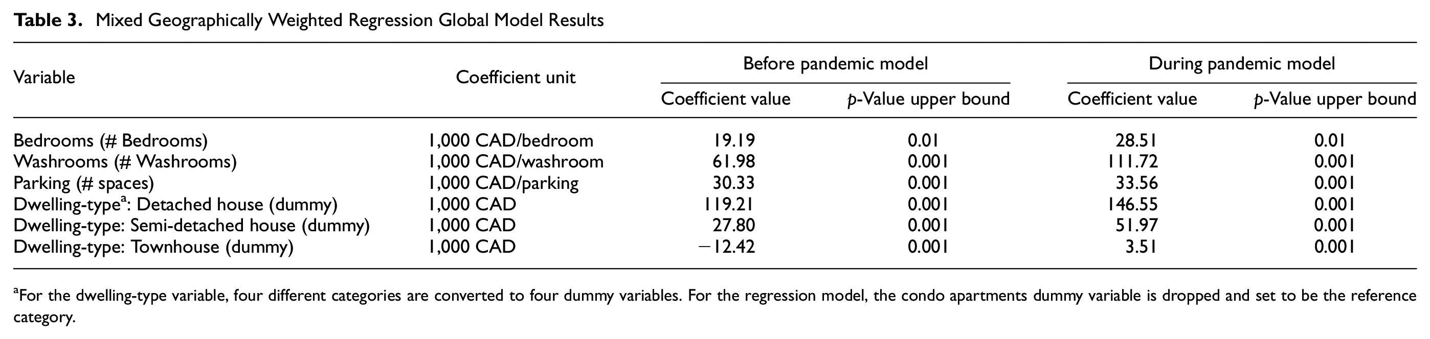
For the dwelling-type variable, four different categories are converted to four dummy variables. For the regression model, the condo apartments dummy variable is dropped and set to be the reference category.
In relation to global results presented in Table 3, a comparison between Tables 2 and 3 reveals that global regression results of the MGWR do not possess the inconsistency of results inherent with the hedonic pricing model. The gained consistency in coefficients is perhaps because of the successful capturing of the dataset’s spatial effects by the MGWR approach. Therefore, unlike the hedonic results in Table 2, the coefficients related to “before the pandemic” and “during the pandemic” are now comparable. Global results suggest an increased interest in purchasing single units compared with multi-unit dwelling types. This finding is consistent with our discussion above, indicating more market activity in suburban areas than urbanized areas. Besides dwelling-type outcomes, dwelling attributes show more weight in buyers’ perceived utility during the pandemic than the previous year.
At the local level, for brevity, not every variable is discussed in this section. In Figures 3 to 7, we discuss variables that demonstrated more spatial variation. Figures which present the results of the other local variables are available on request. Each figure contains two heatmaps; the left heatmap is related to the model fitted on the year before the pandemic dataset. The right figure is related to the pandemic year model. Heatmaps for the same local variables are represented side by side with identical intervals to facilitate the comparison. Figures 3 to 7 show that darker colors in heatmaps indicate larger coefficients, and white circles represent regression points where that local parameter is statistically insignificant. An overall review of Figures 3 to 7 shows suburbanization patterns as more suburban property transactions in the pandemic year than the year before. This pattern could be temporary or lasting depending on the future status of the pandemic and the scale it would affect future daily activities.
Before starting the discussion of the results, we performed another Moran’s I test on the residuals of the MGWR models to ensure this model addresses the spatial autocorrelation in both models. The Moran’s I test on the residuals gave a p-value of 0.376 and 0.230 for the models (before and during the pandemic, respectively), which indicates we cannot reject the null hypothesis of Moran’s I test and that the residuals do not exhibit spatial autocorrelation.
The remainder of this section presents and discusses the estimations of the local parameters. As in the MGWR model, each observation is a regression point, the spatial distributions of parameters are reported in Figures 3 to 7. Therefore, local parameters’ interpretations will be based on the spatial characteristics of the region in relation to the geography of urban form and the transit system. Figure 2 is presented to provide readers with a proper understanding of the geography of the region. In Figure 2, part a, the dwelling densities of the region are provided as a representation of the urban form (Census 2016). In part b of Figure 2, the major transit lines in GTHA regions are demonstrated. The transit network presented in this paper for the GTHA is as follows:
Toronto’s subway system is colored in red (Toronto Transit Commissions subway).
The regional transit system is colored in green (Metrolinx GO transit).
For the rest of the region, on-street transit lines possessing the first quartile transit ridership in the York region (Viva), Mississauga region (MiWay), Hamilton city (HSR) are colored in purple, orange, and blue, respectively.
We start the interpretation of the local parameters with accessibility to regional subway and inter-regional rail transit (Figure 3). Transactions through the year of the pandemic show that proximity to public transit still adds to the value of the dwelling. However, compared with the year before, the value added has noticeably declined, and in some neighbourhoods, the drop is close to 80,000 CAD per subway station within a half-mile. We identify two potential reasons for the observed value decline. The first is the substantial reduction in mobility in the GTA, where the average household trip rate declined from 5.2 to 2.0 ( 42 ). The second is the modal shift from transit to the private car and active modes in the region, which resulted in a sizable drop in transit share from 17.3% to 8% ( 42 ). The drop in the value of accessibility to the subway (i.e., drop in demand for subway proximity) is an immediate effect of mobility changes during the pandemic, and it may have long-term feedback on mobility.
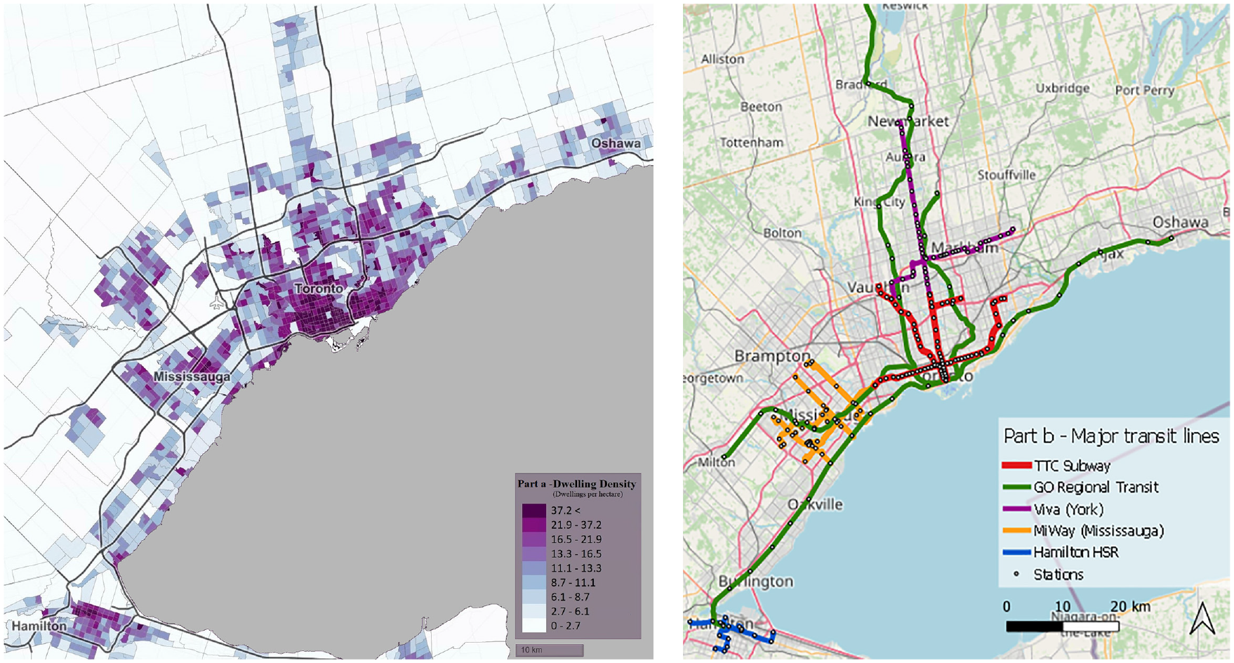
Dwelling densities and major transit lines of the Greater Toronto Hamilton Area.
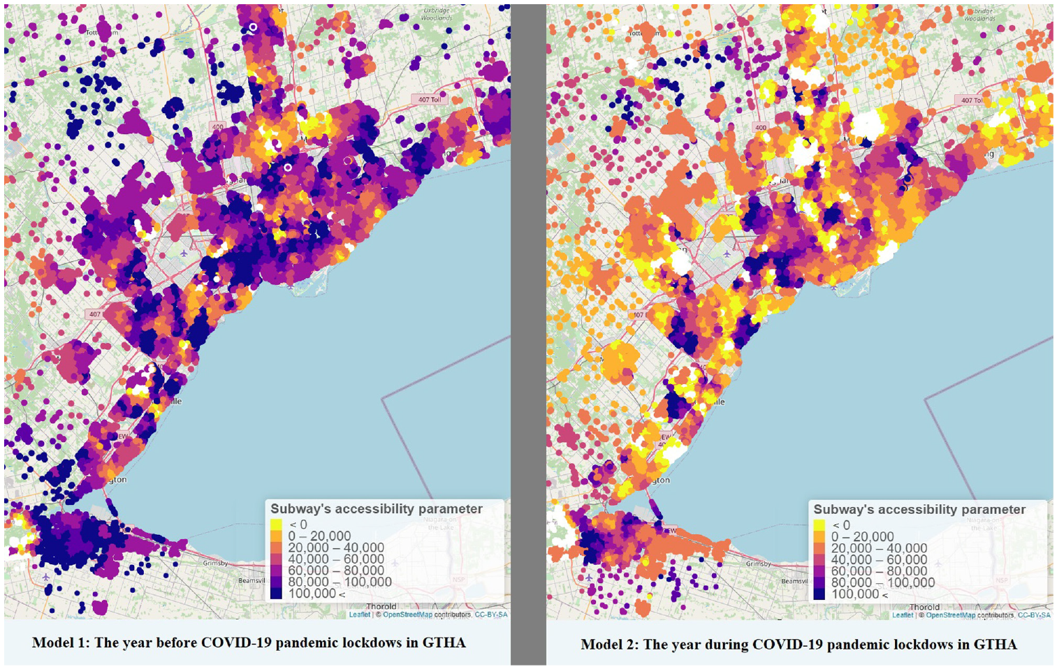
Effect of accessibility to rail transit on residential property values before and during the pandemic.
After all, today’s reduced demand for subway accessibility is tomorrow’s increased demand for non-transit travel modes. Depending on the households’ future adoption rate of ICT choices to substitute their daily activities, the observed suburbanization trend could lead to more driving modes. Our findings for the effect of accessibility to bus and streetcar transit in the region are not like subway accessibility. There are no identifiable patterns in spatial changes in the coefficient of the parameter. We believe that is because most of the properties have immediate access to a bus or streetcar stop in the GTHA area.
Grocery shops are one of the places that did not experience pandemic closures. We were curious to know whether proximity to grocery shops has gained any weight in property demand. As can be seen in Figure 4, the effect of grocery accessibility either before the pandemic or during the pandemic is uncertain. In some cases, the sign of the parameter is positive and, in some cases, negative. No discernable spatial pattern was found for this local variable, and proximity to grocery shops appears to have no bearing on households’ residential preferences. Our findings for accessibility to drugstores are like groceries shops, and households show insensitivity to that factor.
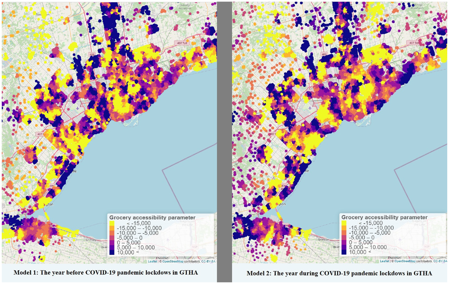
Effect of accessibility to grocery shops on residential property values before and during the pandemic.
Figure 5 shows the spatial distribution of the lot land area local parameter. The unit of area for the coefficient is CAD per square foot of lot area, which can represent the land value. It is essential to check whether there are land value changes in any neighborhood resulting from unobserved factors. For instance, if a neighborhood shows a significant land value change, it is likely that a factor that is not included in our model is causing this change. Having no significant drops or uplifts in land value in Figure 5 is encouraging, as any changes in property price are mostly captured by other variables in both periods.
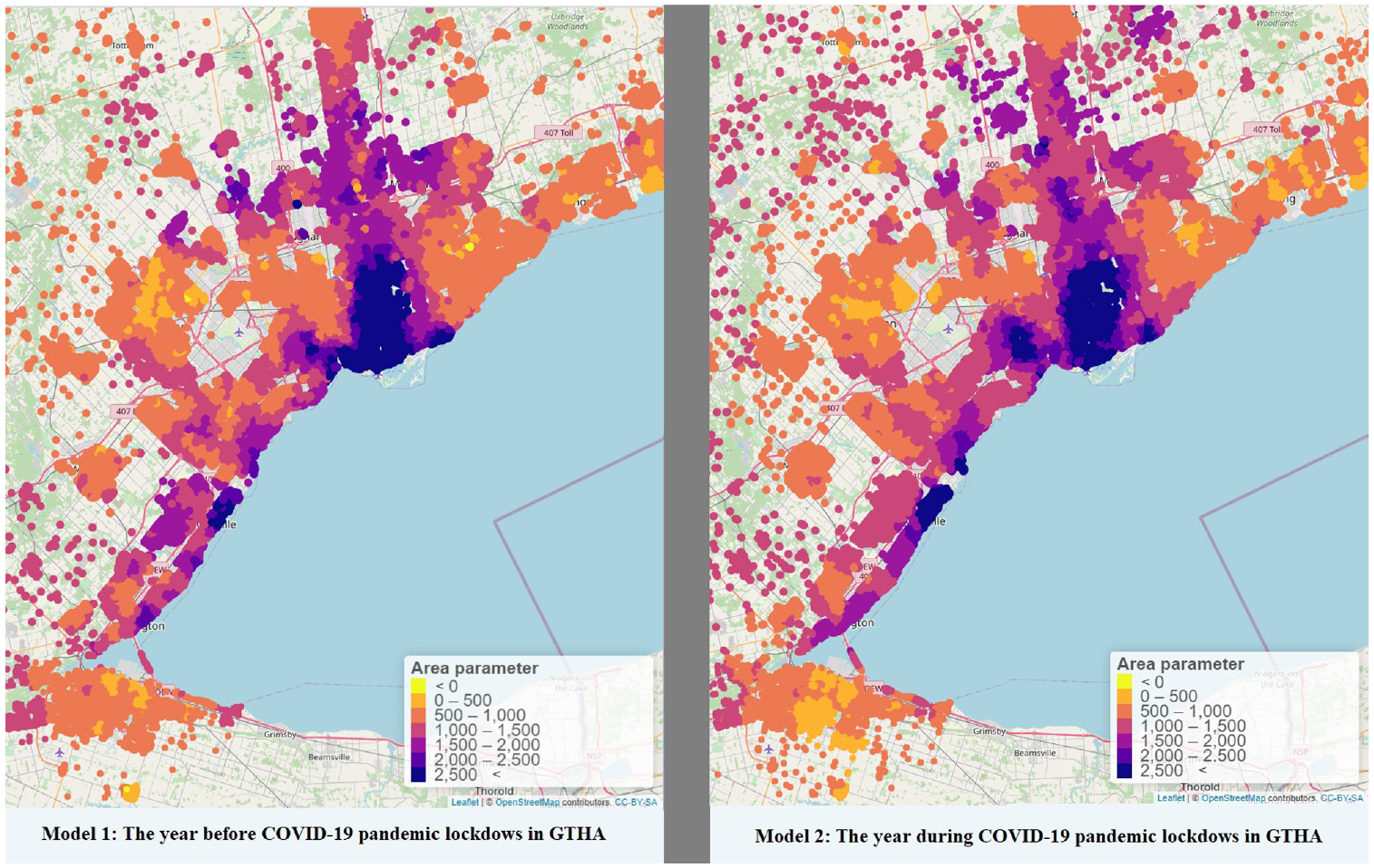
Residential property values before and during the pandemic (CAD per lot sq ft).
Among the most impacted businesses in the GTHA during the pandemic were eating and drinking places. It has been reported that since March 2020, around 205,800 have left the accommodation and food industry because of a lack of job security caused by the pandemic lockdowns ( 43 ). Based on Statistics Canada’s survey, the food and dining industry has been the most affected low-wage industry since the beginning of the pandemic ( 44 ). To answer whether being out of business for most days in the year has any changes in households’ desire for accessibility to those places, and as Figure 6 indicates, the negative impact is minimal in most neighbourhoods. Spatial non-stationary in Figure 6 is more identifiable than any other figure in the paper, which indicates in some regions, households’ accessibility factor to eating and drinking places is different between before and during the COVID-19 pandemic.

Effect of accessibility to drinking and dining places on residential property values before and during the pandemic.
The final variable analyzed in this paper is accessibility to medical clinics (Figure 7). This local parameter is the only parameter that often has a change in sign between years. In some areas, the year before the pandemic, proximity to medical clinics was a bonus and caused value uplift of the property. However, during the pandemic, transactions in the same neighbourhoods negatively affect medical clinic accessibility. Most COVID-19 testing centers in the GTHA are located at hospitals. It is plausible that the previously positive effect of proximity to a medical facility became negative because of a negative association arising from the pandemic.
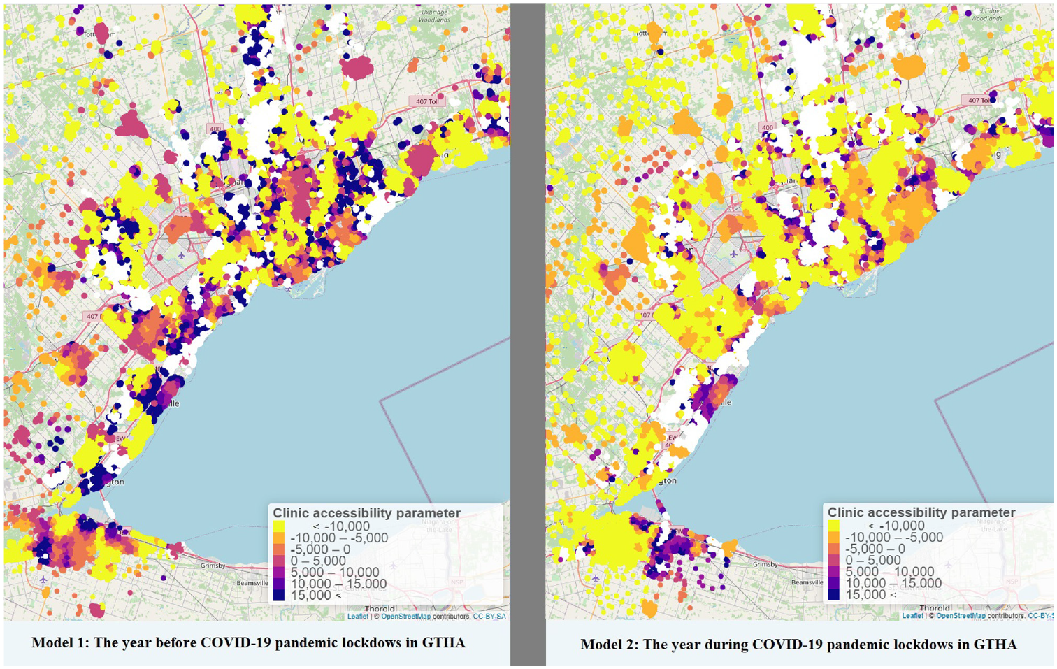
Effect of accessibility to medical clinics on residential property values before and during the pandemic.
Validation of the MGWR Model
After fitting the model on the GTHA dataset, we validated the models estimated using 80% of the population dataset using the remaining 20% of the dataset by analyzing prediction errors.
Sample Size and Prediction Analysis and Goodness of Fit
Previous sections demonstrated how the MGWR model provides better performance to the model’s coefficients descriptive analysis by addressing spatial autocorrelation and spatial non-stationary. In this section, we want to answer whether using MGWR in property accessibility analysis is superior to the simpler hedonic price model in relation to prediction accuracy. We take seven different random samples of 1,000 observations to compare them with a conventional hedonic pricing model to answer this question. For examining the MGWR model goodness of fit and hedonic pricing, we compared the adjusted R-squared for samples and the hedonic pricing model. On average, the R-squared for MGWR models is 0.833, and for the hedonic pricing model, it is 0.616. The average AIC of the MGWR samples is 27,154, and the AIC of the hedonic price model is 27,899 for the same sample size. As shown in Figure 8, results are consistent, and error terms are close to zero. However, in relation to prediction error, the MGWR model for a sample of 1,000 observations does not produce a significant improvement over a hedonic price model. We also include the prediction error for the population-based model, which offers a significant improvement in average prediction error over the sample models.
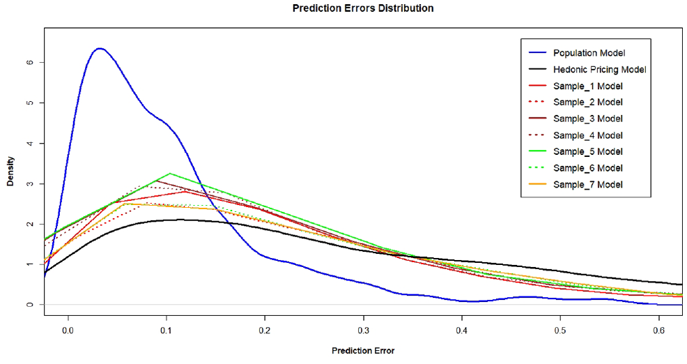
Absolute prediction error comparison between population mixed geographically weighted regression (MGWR), sample MGWR, and conventional hedonic pricing.
The improvement found using the population model raises the question of the relationship between sample size and average prediction error. Figure 9 examines the sensitivity of the MGWR model to sample size. Before discussing the results, it is essential to remind that prediction error density distribution for the hedonic pricing model is similar to that presented in Figure 8, regardless of the sample size. Therefore, the hedonic pricing model is not data sensitive and has greater prediction error because it fails to address spatial effects. Figure 9 shows the MGWR data sensitivity to different sample sizes, thereby reducing the sample size, the prediction accuracy of the model depletes significantly. For our case, around the sample size of 5%, it reaches the performance of the traditional hedonic pricing model. This result suggests that MGWR is not the perfect tool for datasets with smaller sample sizes as the number of regression points will be fewer and reduce the predictive capacity of the MGWR model.
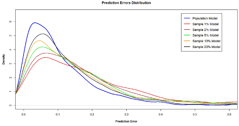
Sample size sensitivity of the mixed geographically weighted regression model.
Conclusions and Future Work
We founded our study on the hypothesis that the budget property purchasers spend for purchasing a residence compensates the utilities they receive from the accessibility the property provides to their activities and dwelling characteristics. We compared MGWR models fitted on data from a year before lockdown restrictions affected GTHA versus the year during the pandemic. Our results show a new balance between the trade-off of dwelling characteristics and accessibility. During the pandemic period, accessibility to subway stations and bus stops added less value to units compared with the year before the pandemic. However, proximity to public transit continues to be perceived as a benefit and increases property value.
In relation to the accessibility to non-transportation points of interest, the results are more nuanced. Some factors such as accessibility to grocery shops and drugstores show a stronger effect on value uplift than the year before the pandemic. On the other hand, some show a change in what factors determine a property’s accessibility in households’ perception. Whether these changes will stay or change once the pandemic is globally over is a research question that requires more data and time to be answered.
A significant shift has occurred in the housing market in relation to increased detached units’ values and reduced condo and townhouses values. This indicates an increase in demand for single-unit residences in contrast to multi-unit residences through the pandemic year. Our finding is consistent with the recent report on vacancy rates in the region, which indicates that vacancy rates of central areas have increased despite the decreasing rates in suburban areas ( 45 ). The current housing market behaviour is contrary to compact urban development goals in the region. Still, the housing market may go back to its previous trend once the pandemic is over, but this should be considered an initial warning for the region.
The new ICT-oriented pandemic lifestyle’s footprint is also trackable in the housing market. Households’ perception of the utility of dwelling characteristics shows more weight compared with accessibility measures in the model during the pandemic. Perhaps this change is because nowadays households spend more time in their residence and have a higher demand for better quality, but potentially less accessible, dwellings relative to the pattern found in the model of the pre-pandemic year.
The MGWR model captured all existing spatial effects in our datasets and vividly described the relations between transportation accessibility and dwellings’ characteristics. In relation to the predictive capacity of the chosen methodology, because of the number of regressions for estimation, MGWR is very data-intensive, and prediction accuracy is mainly dependent on the sample size. Although MGWR is very good at handling spatial effects in the dataset, it is not recommended for studies where the availability of the housing transaction dataset is limited or unreliable.
This study has limitations such as the lack of information on who purchased the properties, what other options they had in the market, and where the common destinations of households’ daily activities are. For future works, a complementary study can be devised to fuse the regional demographic and origin–destination dataset to the housing market dataset for a more comprehensive accessibility analysis. We do not recommend the use of MGWR methodologies for the studies that have access to less than 5% of the whole population as it does not demonstrate superiority to the traditional hedonic pricing model. It would also be useful to perform a similar exercise on sample size and repeated sampling using other spatial models to test their data intensiveness.
Footnotes
Author Contributions
The authors confirm contribution to the paper as follows: study conception and design: S. Shakib; data collection: S. Shakib; analysis and interpretation of results: S. Shakib, J. Hawkins, and K. M. N. Habib; draft manuscript preparation: S. Shakib, J. Hawkins, and K. M. N. Habib. All authors reviewed the results and approved the final version of the manuscript.
Declaration of Conflicting Interests
The author(s) declared no potential conflicts of interest with respect to the research, authorship, and/or publication of this article.
Funding
The author(s) disclosed receipt of the following financial support for the research, authorship, and/or publication of this article: The study was funded by an NSERC Discovery grant.
Data Accessibility Statement
Data analyzed in this study were a re-analysis of existing data, which are either publicly available or available from third parties. The General Transit Feed Specification (GTFS) dataset is publicly available through each municipality’s website. Other data sources implemented in this study are available from Toronto Regional Real Estate Board (TRREB), Information Technology Systems Ontario (ITSO), DMTI Spatial Company with permissions and/or license. Authors are unable to provide non-publicly available datasets used in this study because of third party restrictions.