Sage Journals: Discover world-class research

Abstract

Decision-makers in synchromodal transport (ST) have different preferences toward different objectives, such as cost, time, and emissions. To solve the conflicts among objectives and obtain preferred solutions, a preference-based multi-objective optimization model is developed. In ST, containers need to be transferred across modes, therefore the optimization problem is formulated as a pickup and delivery problem with transshipment. The preferences of decision-makers are usually expressed in linguistic terms, so weight intervals, that is, minimum and maximum weights, are assigned to objectives to represent such vague preferences. An adaptive large neighborhood search is developed and used to obtain non-dominated solutions to construct the Pareto frontier. Moreover, synchronization is an important feature of ST and it makes available resources fully utilized. Therefore, four synchronization cases are identified and studied to make outgoing vehicles cooperate with changes of incoming vehicles’ schedules at transshipment terminals. Case studies in the Rhine-Alpine corridor are designed and the results show that the proposed approach provides non-dominated solutions which are in line with preferences. Moreover, the mode share under different preferences is analyzed, which signals that different sustainability policies in transportation will influence the mode share.

Keywords

freight systems intermodal freight transport multimodal optimization planning and logistics container logistic

With the growth of international trade in recent decades, the use of intermodal transportation is increasing because of its positive impacts on economics and the environment ( 1 , 2 ). Intermodal transport means freight transported by at least two modes, for example, barge, train, and truck. Trucks are fast and flexible but with high carbon emissions, while trains are slow with low carbon emissions. Barges are also slow but are good with both low cost and low carbon emissions ( 3 ). Synchromodal transport (ST) is the newest concept in the conceptual evolution of intermodal transport, which optimally uses all kinds of available resources and selects transport routes/modes at any time based on the operational circumstances, customer requirements, or both ( 1 , 4 ).

In ST, carriers (operators of vehicles) have different preferences toward different objectives according to the requirements of shippers (owners or suppliers of containers). Typically, the primary objective of carriers is to minimize the transport cost. Transport time also plays an important role in transport route optimization because it influences both cost and reliability. Moreover, the government stimulates stakeholders to minimize the total $C O_{2}$ emissions. To achieve ST, it is necessary to consider multiple objectives and preferences and synthesize the best attributes of different modes in the optimization model for carriers. As shown in Figure 1, the carrier needs to find the most appropriate routes of multiple modes, including barges, trains, and trucks, according to their preferences. Moreover, as a distinct feature of ST, synchronization, that is, coordination of involved operations, is needed because transshipment makes vehicles dependent on each other ( 5 ). For example, when the carrier needs to transport perishable cargoes for shippers, the time objective is important and the proportion of fast modes (such as trains and trucks) in transport planning will be higher. However, in the ST literature, most scholars ignore the different objectives and preferences of carriers ( 6 , 7 ).

Figure 1.

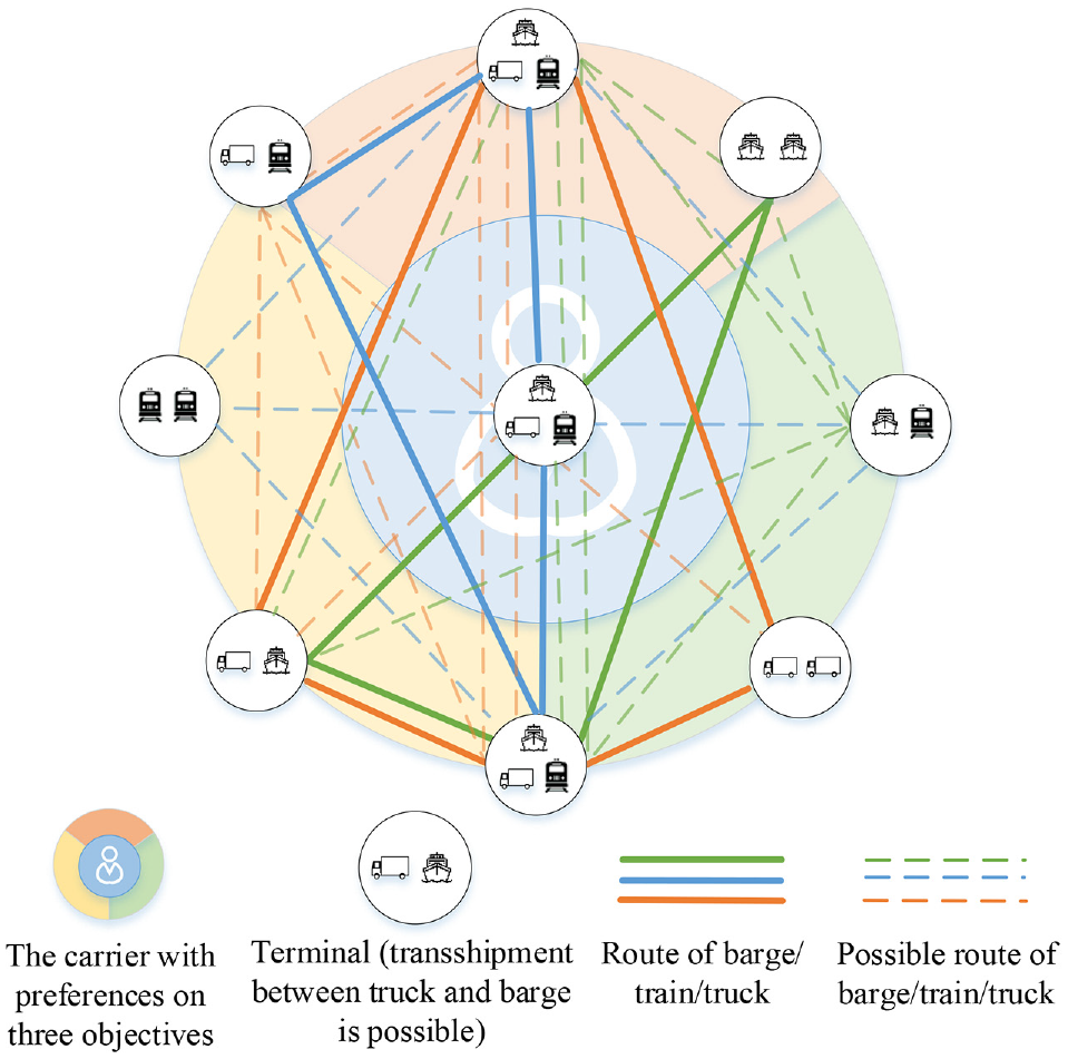
Vehicle routing for synchromodal transport considering preferences and synchronization.

To address the above gaps, this work introduces a preference-based multi-objective optimization model for ST. The optimization problem is formulated as a pickup and delivery problem with transshipment (PDPT), and an adaptive large neighborhood search (ALNS) is developed to solve it. The remainder of this paper is structured as follows. The second section presents a brief literature review which is followed by problem description and mathematical model. Next, the solution methodology is presented, after which experimental settings and results are provided. The final section concludes the paper and gives future research directions.

Literature Review

This paper studies transshipment, synchronization, and preferences-based multi-objective optimization in ST. Therefore, the presented literature review focuses on these three distinctive aspects as well as literature that studies multi-objective optimization for intermodal transport.

Transshipment

A distinctive feature of intermodal transport is the transshipment between modes/vehicles. To model transshipment, most scholars use the network flow (NF) model, in which commodity flows are covered by arcs and paths (a series of arcs) of the transport network rather than routes of vehicles ( 1 ). The type of vehicles used can be then ignored and containers can be transferred freely in nodes of the network. The advantage of this approach is that the computation time is relatively short. However, these studies lack a direct vehicle routing component ( 8 ). Compared with the NF model, optimizing both container and vehicle routing brings three benefits:

Capacity constraints and time constraints can be used on vehicles rather than services, which is more accurate.

In the NF model, containers can only be transported on the predefined arc. If the vehicle routing is considered, the containers can change routes on nodes of the arc, which is more flexible.

The optimization results can provide the routing plan to vehicles directly, which is more practical.

Transshipment between vehicles is also a common practice in other transportation operations and is considered in various modeling approaches, including vehicle routing problem with trailers and transshipment ( 9 ), vehicle routing problem with cross-docking ( 10 ), and PDPT ( 11 ). PDPT is suitable for ST. Thus this research studies PDPT for ST, considering both container routing and vehicle routing.

In a previous paper ( 12 ), the authors proposed an optimization model for PDPT in inland waterway transport. There are three main differences between Zhang et al. ( 12 ) and this paper: (a) Zhang et al. ( 12 ) only optimized the routing of barges, while this paper considers multiple modes; (b) this paper takes preferences into account, which is not considered by Zhang et al. ( 12 ); (c) specific synchronization cases are presented in this paper, and they are not illustrated in Zhang et al. ( 12 ).

Synchronization

To use the available resources optimally, synchronization is a key factor in optimization for ST ( 5 ). In the standard vehicle routing problem (VRP), vehicles are independent of one another. For example, removing a request from one route does not affect any other route before this request is inserted into routes again. In ST, by contrast, a change in one route may have effects on other routes even though no request is removed or added. For example, removing request 1 from a route of vehicle $k$ means that vehicle $k$ will deliver request 2 at the transshipment terminal earlier than the scheduled time, but vehicle $l$ , which will pick up request 2 at the transshipment terminal, has not arrived. Therefore, vehicle $l$ needs to change its route to adapt to the new situation, otherwise request 2 needs to be stored at the transshipment terminal with a storage fee. In the worst case, a change in one route may render all other routes infeasible. This is called the interdependence problem ( 8 ). Therefore the synchronization among vehicles is crucial for the optimization of ST. Behdani et al. ( 13 ) also point out that including synchronization in the optimization process could improve transportation performance.

Synchronization in VRP has been studied in the literature. According to Drexl ( 8 ), the following types of problems need to consider synchronization:

Pickup and delivery problem with split loads ( 14 ).

VRP with transshipment of loads or transfer of persons ( 15 ).

The requirement of simultaneous presence of vehicles at a location to render a service ( 16 ).

The existence of nonautonomous vehicles ( 17 ).

The problem in this research belongs to the second type: VRP with transshipment of loads. Although many studies have contributed to synchronization in VRP, to the best of the authors’ knowledge, synchronization has not been studied fully in ST ( 5 ).

Preference-Based Multi-Objective Optimization

Wang et al. ( 18 ) provide a summary of methods on how to incorporate preferences into multi-objective optimization (MOO), such as weight sum method, reference point, reference direction, utility function, and so forth. According to Coello et al. ( 19 ), preference-based MOO approaches are divided into three categories: priori ( 20 , 21 ), progressive ( 22 , 23 ), and posteriori ( 24 ) preference articulations, which mean making decisions before, during, and after search, respectively. In ST, it may be impractical for a decision-maker (DM) to specify their preferences completely before any alternatives are known. However, the DM has at least a rough idea about the reasonable trade-offs between different objectives, which is termed vague preferences. For example, Szlapczynska and Szlapczynski ( 20 ) propose a MOO model in ship weather routing, considering vague preferences of DMs in the form of weight intervals. Therefore, the priori preference articulations approach is used in this paper and Pareto optimal solutions are obtained according to preferences.

The $ε$ -constraint method is often used for multi-objective problems; it is based on minimizing/maximizing one of the objectives and restricting the rest of the objectives within predefined values ( 3 ). For heuristic approaches, evolutionary algorithms, such as NSGA-2 (Nondominated Sorting Genetic Algorithm II) ( 25 ), are often used in MOO problems. Besides evolutionary algorithms, ALNS can also be used to solve the MOO problem. ALNS is more suitable for this study because it has been successfully applied to VRP and performs robustly on different instances because of its adaptive nature ( 11 ).

MOO for Intermodal Transport

Two types of problems are considered in the literature. The service network design problem relates to choosing services and optimizing vehicle frequencies in the transport network. Route optimization involves the planning decisions of routes and modes. The methods for solving MOO used in different studies are different. Table 1 provides a summary of models in the literature to position the present work. As mentioned above, the vehicle routing component has many benefits; taking synchronization into account is conducive to making full use of limited resources, and considering preferences is important to solve the conflicts among objectives. However, vehicle routing, synchronization, and preferences are rarely considered in the literature and these are the core contributions of this paper. Furthermore, an ALNS algorithm is used to solve the problem, and the procedures within ALNS are tailored to be specific to the synchromodal case which is another distinction of this paper.

Table 1.

Comparison of Models in the Literature

Article	Problem definition	Objectives	Vehicle routing	Synchronization	Preferences	Solution method
Kalinina et al. ( 3 )	SND	c, e, t	×	×	×	$ε$
Xiong and Wang ( 26 )	RO	c, t	×	×	×	GA
Baykasoglu and Subulan ( 27 )	SND	c, e, t	×	×	✓	CP, FGP
Ji and Luo ( 28 )	SND	c, t	×	×	×	HEDA
Mnif and Bouamama ( 29 )	SND	c, t	×	×	×	FA
Chen et al. ( 30 )	RO	c, t, cc	×	×	×	NNCM
This paper	RO	c, e, t	✓	✓	✓	ALNS

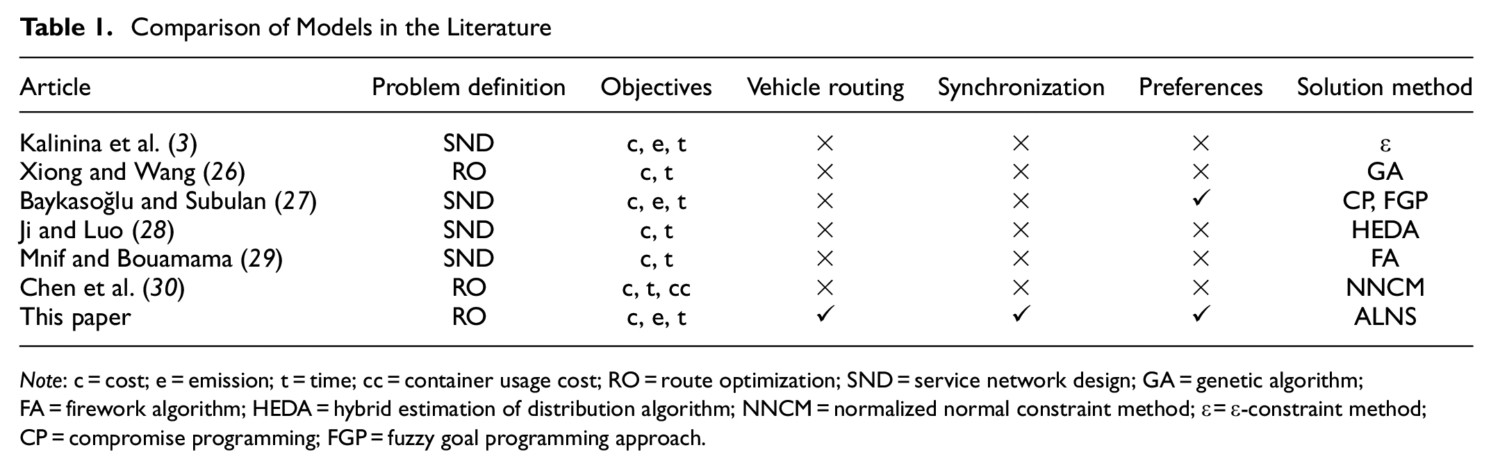
Note: c = cost; e = emission; t = time; cc = container usage cost; RO = route optimization; SND = service network design; GA = genetic algorithm; FA = firework algorithm; HEDA = hybrid estimation of distribution algorithm; NNCM = normalized normal constraint method; $ε$ = $ε$ -constraint method; CP = compromise programming; FGP = fuzzy goal programming approach.

Problem Description

The main research question of this study is: How can ST be optimized according to the preferences of the carrier? To answer this research question, three key research problems need to be solved, as shown in Figure 2:

Compared with unimodal transport, ST is more complex because multiple modes are used and transshipment is needed between modes/vehicles. As illustrated in the literature review, considering both container routing and vehicle routing in transshipment modeling makes the optimization more accurate, more flexible, and more practical. To add vehicle routing into the model, the following research questions need to be answered: How to optimize container routing and vehicle routing simultaneously? How to model the transshipment with both vehicle and container constraints?

Compared with intermodal transport, synchronization should be taken into account because of the synchromodality requirements in ST. Because of the transshipment, the route planning of a vehicle in ST may depend on the route planning of other vehicles. With regard to the optimization problem, a PDPT only makes the transshipment possible, but does not make full use of transshipment because many solutions are infeasible without synchronization. By coordinating vehicles, synchronization takes full advantage of serving a request by multiple vehicles/modes in ST. The following research questions need to be considered in the synchronization: Is the vehicle dependent on one vehicle or multiple vehicles? How do the vehicles coordinate when they are dependent on each other? Is there an infeasible solution no matter how the vehicles are coordinated?

Compared with single-objective optimization, conflicts between objectives need to be considered in the MOO. By taking preferences into account, the problem may be addressed. As mentioned above, in ST DMs usually cannot provide accurate preferences. Therefore, we should consider first how to represent the vague preferences of DMs. Then, how to incorporate preferences into the optimization model is another problem to consider.

Solving Problem 1 (P1) is the basis for solving Problem 2 (P2) and Problem 3 (P3). All methods for these problems are used to establish the preference-based MOO model for ST, which will be used to obtain attractive solutions for DMs.

Figure 2.

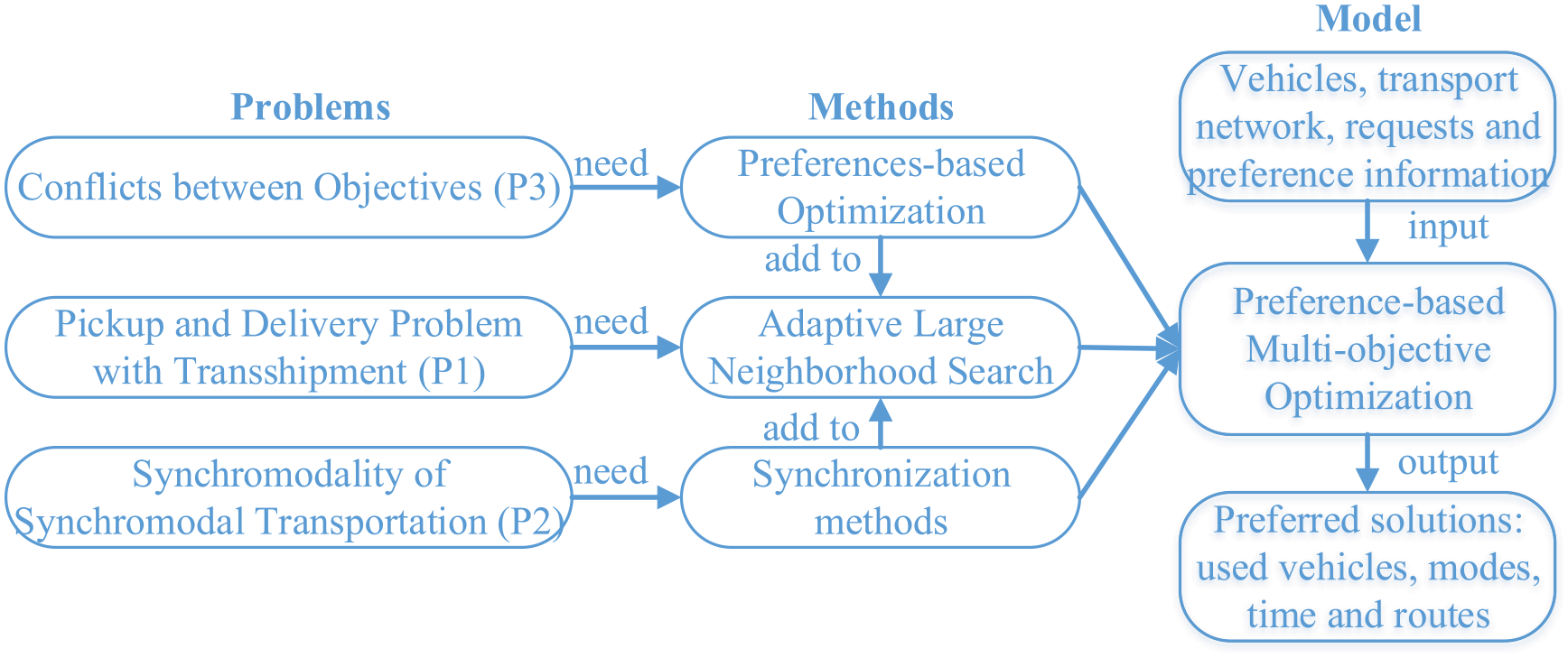
Key research problems in this study.

Mathematical Model

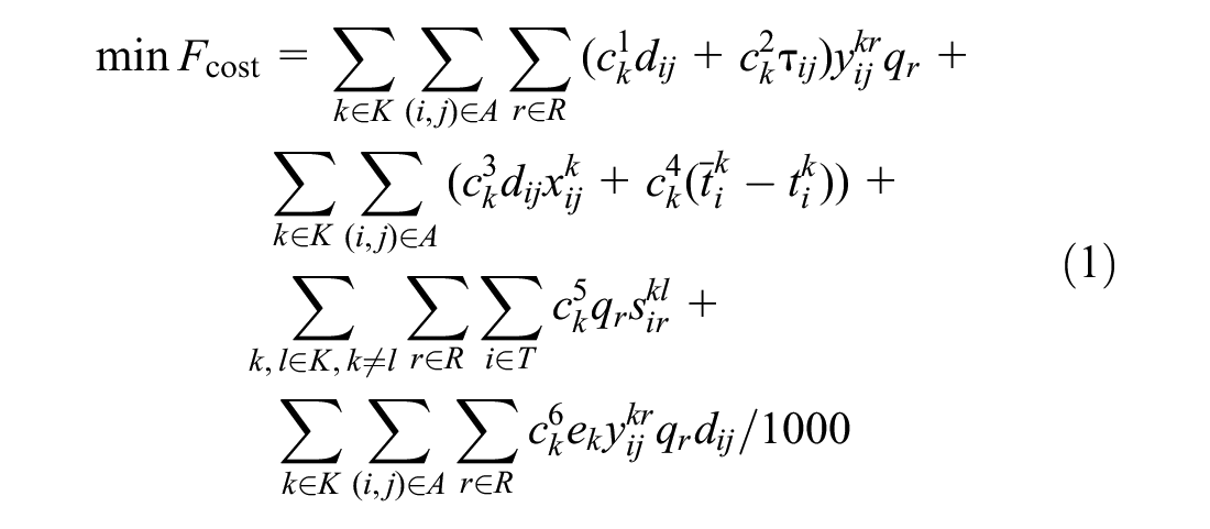
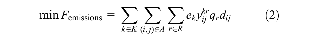
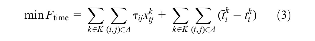
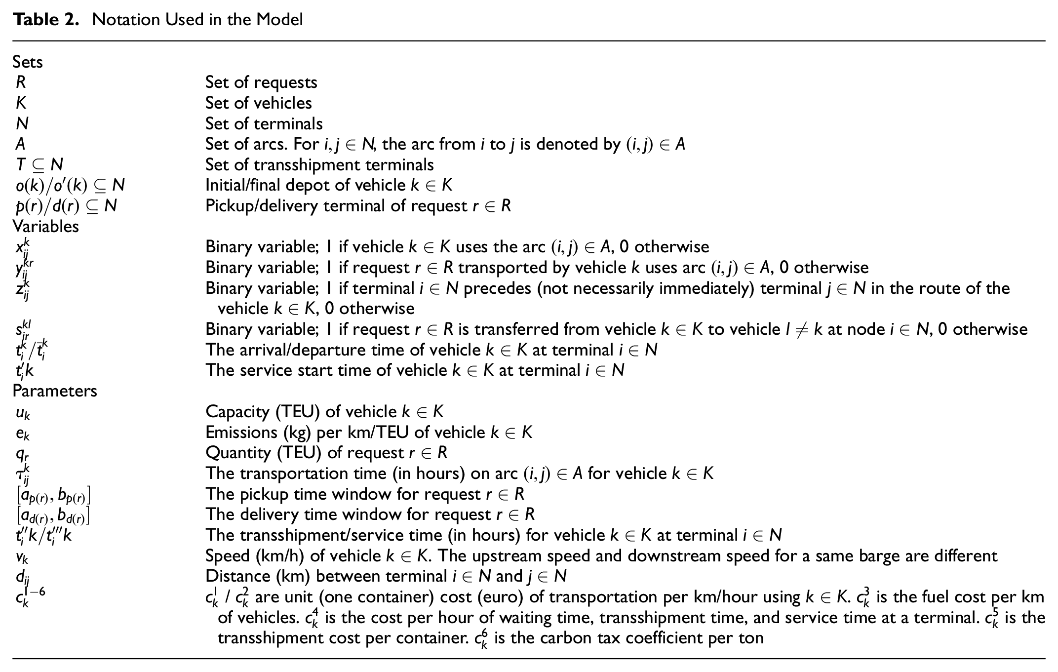
The notations of the mathematical model are given in Table 2. A MOO model for the PDPT in ST is given by Equations 1–32 as described below. Three objectives, that is, minimizing cost, emissions, and time, are considered, as Equations 1–3 show. The cost objective consists of transportation cost of containers, fuel cost, transshipment cost, and cost associated with waiting, service, and transshipment time. “Emissions” in this paper refers to CO₂ emissions. There are different ways to calculate such emissions in the literature ( 31 ), and the activity-based method is one of the popular methods because activity data is easier to obtain compared with other methods ( 32 , 33 ). Therefore this work uses the activity-based method and calculation of CO₂ emissions based on vehicle type, distance, and amount of containers ( 34 ). For different modes the emissions factor $e_{k}$ is different and detailed data are shown in the Case Study section. The time objective includes the time on the route and waiting time at terminals. Because this paper considers vehicle, container routing, and transshipment, both vehicle and container flows are modeled and transshipment constraints are designed, which are illustrated in detail in Equations 4–32.

\begin{matrix} \min F_{cost} = \sum_{k \in K} \sum_{(i, j) \in A} \sum_{r \in R} (c_{k}^{1} d_{ij} + c_{k}^{2} τ_{ij}) y_{ij}^{kr} q_{r} + \\ \sum_{k \in K} \sum_{(i, j) \in A} (c_{k}^{3} d_{ij} x_{ij}^{k} + c_{k}^{4} ({\bar{t}}_{i}^{k} - t_{i}^{k})) + \\ \sum_{k, l \in K, k \neq l} \sum_{r \in R} \sum_{i \in T} c_{k}^{5} q_{r} s_{ir}^{kl} + \\ \sum_{k \in K} \sum_{(i, j) \in A} \sum_{r \in R} c_{k}^{6} e_{k} y_{ij}^{kr} q_{r} d_{ij} / 1000 \end{matrix}

(1)

\min F_{emissions} = \sum_{k \in K} \sum_{(i, j) \in A} \sum_{r \in R} e_{k} y_{ij}^{kr} q_{r} d_{ij}

(2)

\min F_{time} = \sum_{k \in K} \sum_{(i, j) \in A} τ_{ij} x_{ij}^{k} + \sum_{k \in K} \sum_{(i, j) \in A} ({\bar{t}}_{i}^{k} - t_{i}^{k})

(3)

Table 2.

Notation Used in the Model

Sets
$R$	Set of requests
$K$	Set of vehicles
$N$	Set of terminals
$A$	Set of arcs. For $i, j \in N$ , the arc from $i$ to $j$ is denoted by $(i, j) \in A$
$T \subseteq N$	Set of transshipment terminals
$o (k) / o' (k) \subseteq N$	Initial/final depot of vehicle $k \in K$
$p (r) / d (r) \subseteq N$	Pickup/delivery terminal of request $r \in R$
Variables
$x_{ij}^{k}$	Binary variable; 1 if vehicle $k \in K$ uses the arc $(i, j) \in A$ , 0 otherwise
$y_{ij}^{kr}$	Binary variable; 1 if request $r \in R$ transported by vehicle $k$ uses arc $(i, j) \in A$ , 0 otherwise
$z_{ij}^{k}$	Binary variable; 1 if terminal $i \in N$ precedes (not necessarily immediately) terminal $j \in N$ in the route of the vehicle $k \in K$ , 0 otherwise
$s_{ir}^{kl}$	Binary variable; 1 if request $r \in R$ is transferred from vehicle $k \in K$ to vehicle $l \neq k$ at node $i \in N$ , 0 otherwise
$t_{i}^{k} / {\bar{t}}_{i}^{k}$	The arrival/departure time of vehicle $k \in K$ at terminal $i \in N$
$t'_{i}^{k}$	The service start time of vehicle $k \in K$ at terminal $i \in N$
Parameters
$u_{k}$	Capacity (TEU) of vehicle $k \in K$
$e_{k}$	Emissions (kg) per km/TEU of vehicle $k \in K$
$q_{r}$	Quantity (TEU) of request $r \in R$
$τ_{ij}^{k}$	The transportation time (in hours) on arc $(i, j) \in A$ for vehicle $k \in K$
$[a_{p (r)}, b_{p (r)}]$	The pickup time window for request $r \in R$
$[a_{d (r)}, b_{d (r)}]$	The delivery time window for request $r \in R$
${t^{″}}_{i}^{k} / {t^{'″}}_{i}^{k}$	The transshipment/service time (in hours) for vehicle $k \in K$ at terminal $i \in N$
$v_{k}$	Speed (km/h) of vehicle $k \in K$ . The upstream speed and downstream speed for a same barge are different
$d_{ij}$	Distance (km) between terminal $i \in N$ and $j \in N$
$c_{k}^{1 - 6}$	$c_{k}^{1}$ / $c_{k}^{2}$ are unit (one container) cost (euro) of transportation per km/hour using $k \in K$ . $c_{k}^{3}$ is the fuel cost per km of vehicles. $c_{k}^{4}$ is the cost per hour of waiting time, transshipment time, and service time at a terminal. $c_{k}^{5}$ is the transshipment cost per container. $c_{k}^{6}$ is the carbon tax coefficient per ton

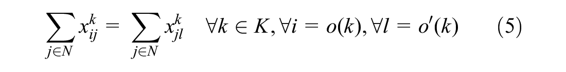
Constraints (4)–(21) are the spatial constraints. Constraints (4)–(11) are typical constraints in PDP. Constraints (4) and (5) ensure that a vehicle begins and ends at its begin and end depot, respectively. Constraints (6) and (7) ensure that containers for each request must be picked and delivered at its pick up and delivery terminal, respectively. Constraints (8)–(10) are the subtour elimination constraints, which provide tight bounds among several polynomial-size versions of subtour elimination constraints ( 35 ). Constraint (11) is the capacity constraint.

\sum_{j \in N} x_{ij}^{k} \leq 1 \forall k \in K, \forall i = o (k)

(4)

\sum_{j \in N} x_{ij}^{k} = \sum_{j \in N} x_{jl}^{k} \forall k \in K, \forall i = o (k), \forall l = o' (k)

(5)

\sum_{k \in K} \sum_{j \in N} y_{ij}^{kr} = 1 \forall r \in R, \forall i = p (r)

(6)

\sum_{k \in K} \sum_{j \in N} y_{ji}^{kr} = 1 \forall r \in R, \forall i = d (r)

(7)

x_{ij}^{k} \leq z_{ij}^{k} \forall i, j \in N, \forall k \in K

(8)

z_{ij}^{k} + z_{ji}^{k} = 1 \forall i, j \in N, \forall k \in K

(9)

z_{ij}^{k} + z_{jl}^{k} + z_{li}^{k} \leq 2 \forall i, j, l \in N, \forall k \in K

(10)

\sum_{r \in R} q_{r} y_{ij}^{kr} \leq u_{k} x_{ij}^{k} \forall (i, j) \in A, \forall k \in K

(11)

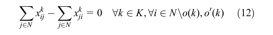
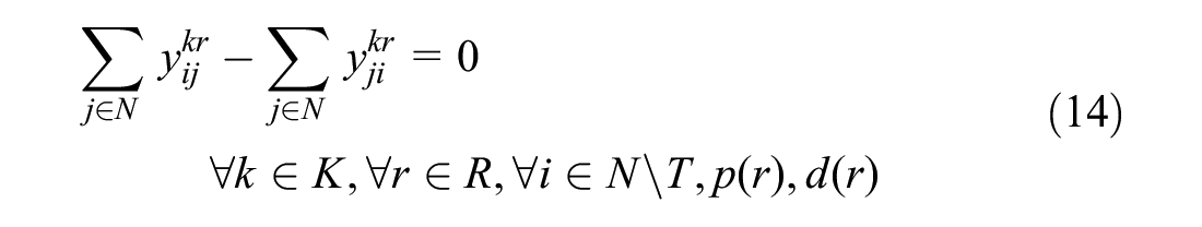
Flow conservation constraints of both vehicles and requests are handled by Constraints (12)–(15). Constraint (12) represents flow conservation for vehicle flow and (13)–(14) represent flow conservation for request flow. Constraint (13) is for transshipment terminals, and Constraint (14) is for regular terminals. Constraint (15) links $y$ and $x$ variables to guarantee that, for a request to be transported by a vehicle, that vehicle needs to be traversing the associated arc.

\sum_{j \in N} x_{ij}^{k} - \sum_{j \in N} x_{ji}^{k} = 0 \forall k \in K, \forall i \in N \ o (k), o' (k)

(12)

\begin{matrix} \sum_{k \in K} \sum_{j \in N} y_{ij}^{kr} - \sum_{k \in K} \sum_{j \in N} y_{ji}^{kr} = 0 \\ \forall r \in R, \forall i \in T \ p (r), d (r) \end{matrix}

(13)

\begin{matrix} \sum_{j \in N} y_{ij}^{kr} - \sum_{j \in N} y_{ji}^{kr} = 0 \\ \forall k \in K, \forall r \in R, \forall i \in N \ T, p (r), d (r) \end{matrix}

(14)

y_{ij}^{kr} \leq x_{ij}^{k} \forall (i, j) \in A, \forall k \in K, \forall r \in R

(15)

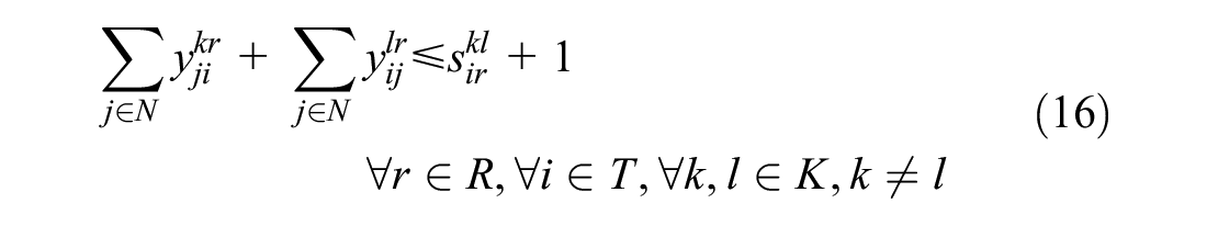
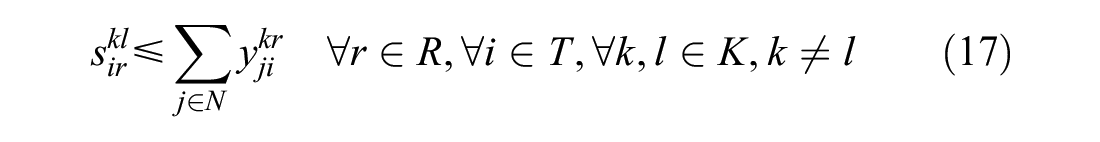
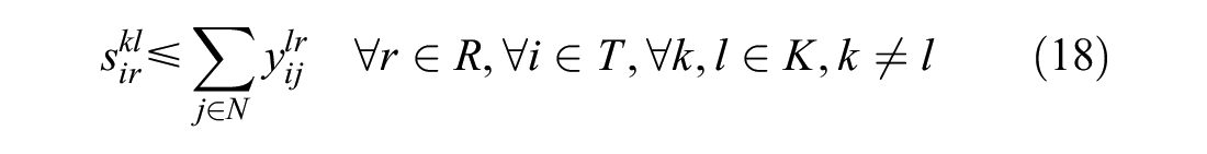
Constraints (16)–(18) facilitate transshipment. Constraint (16) ensures that the transshipment occurs only once in the transshipment terminal. Furthermore, Constraints (17) and (18) allow the transshipment only when the request is transported by both vehicles $k$ and $l$ .

\begin{matrix} \sum_{j \in N} y_{ji}^{kr} + \sum_{j \in N} y_{ij}^{lr} \leq s_{ir}^{kl} + 1 \\ \forall r \in R, \forall i \in T, \forall k, l \in K, k \neq l \end{matrix}

(16)

s_{ir}^{kl} \leq \sum_{j \in N} y_{ji}^{kr} \forall r \in R, \forall i \in T, \forall k, l \in K, k \neq l

(17)

s_{ir}^{kl} \leq \sum_{j \in N} y_{ij}^{lr} \forall r \in R, \forall i \in T, \forall k, l \in K, k \neq l

(18)

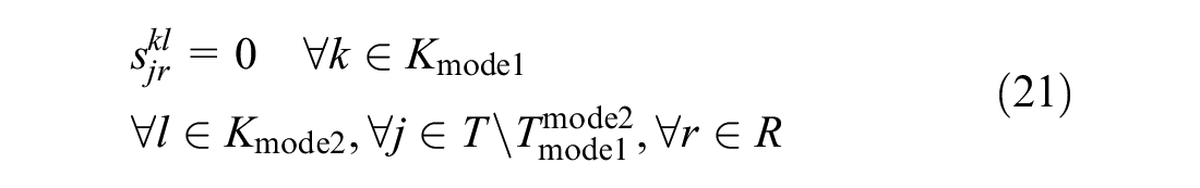
Characteristics of ST are considered in Constraints (19)–(21). Constraint (19) avoids vehicles running on unsuitable routes, for example, trucks cannot run on inland waterways. Constraint (20) takes care of predefined routes for certain vehicles, for example, trains have fixed routes and terminals. Constraint (21) ensures the transshipment occurs in the right transshipment terminal, because some transshipment terminals only allow the transshipment between two specific modes. When containers need to be transferred from barges to trucks, terminals that only allow transshipment between barges and trains will not be considered.

x_{ij}^{k} = 0 \forall k \in K_{mode} \forall (i, j) \in A \ A_{mode}

(19)

x_{ij}^{k} = 0 \forall k \in K_{certain} \forall (i, j) \in A \ A_{predefined}

(20)

\begin{matrix} s_{jr}^{kl} = 0 \forall k \in K_{mode 1} \\ \forall l \in K_{mode 2}, \forall j \in T \ T_{mode 1}^{mode 2}, \forall r \in R \end{matrix}

(21)

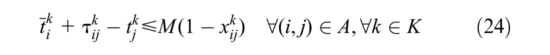
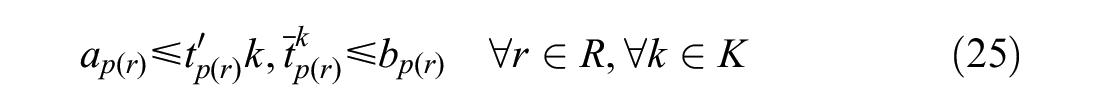
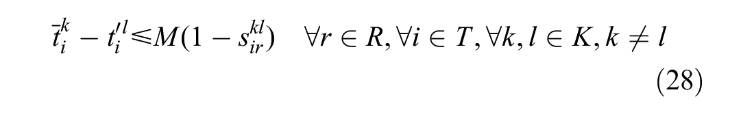
Constraints (22)–(30) are the temporal constraints. Constraint (22) guarantees that the arrival time of vehicle is earlier than the service start time. Constraint (23) maintains that the departure happens only after the service is completed. Constraint (24) ensures that the time on the route is consistent with the distance traveled and speed, and that $M$ is a large enough positive number. Constraints (25) and (26) take care of the time windows. These constraints give the possibility of waiting at terminals when a vehicle arrives earlier. Constraint (27) adds the service time of pickup and delivery.

t_{i}^{k} \leq t'_{i}^{k} \forall i \in N, \forall k \in K

(22)

t'_{i}^{k} \leq {\bar{t}}_{i}^{k} \forall i \in N, \forall k \in K

(23)

{\bar{t}}_{i}^{k} + τ_{ij}^{k} - t_{j}^{k} \leq M (1 - x_{ij}^{k}) \forall (i, j) \in A, \forall k \in K

(24)

a_{p (r)} \leq t'_{p (r)}^{k}, {\bar{t}}_{p (r)}^{k} \leq b_{p (r)} \forall r \in R, \forall k \in K

(25)

a_{d (r)} \leq t'_{d (r)}^{k}, {\bar{t}}_{d (r)}^{k} \leq b_{d (r)} \forall r \in R, \forall k \in K

(26)

t'_{p (r) / d (r)}^{k} + t ″'_{p (r) / d (r)}^{k} = {\bar{t}}_{p (r) / d (r)}^{k} \forall r \in R, \forall k \in K

(27)

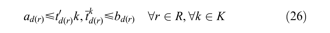
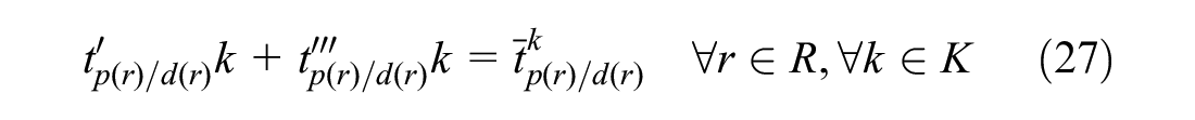
Constraints (28)–(30) include time constraints for transshipment. If there is a transshipment from vehicle $k$ to vehicle $l$ , but vehicle $l$ arrives before vehicle $k$ departs, then Constraint (28) allows vehicle $l$ to wait until vehicle $k$ completes its unloading. Constraints (29) and (30) add transshipment time at the transshipment terminal.

{\bar{t}}_{i}^{k} - {t^{'}}_{i}^{l} \leq M (1 - s_{ir}^{kl}) \forall r \in R, \forall i \in T, \forall k, l \in K, k \neq l

(28)

{\bar{t}}_{i}^{k} - {t^{'}}_{i}^{k} = {t^{″}}_{i}^{k} s_{ir}^{kl} \forall r \in R, \forall i \in T, \forall k, l \in K, k \neq l

(29)

{\bar{t}}_{i}^{l} - {t^{'}}_{i}^{l} = {t^{″}}_{i}^{l} s_{ir}^{kl} \forall r \in R, \forall i \in T, \forall k, l \in K, k \neq l

(30)

Constraints (31) and (32) set variables $x$ and $y$ as binary variables.

x_{ij}^{k} \in {0, 1} \forall (i, j) \in A, \forall k \in K

(31)

y_{ij}^{kr} \in {0, 1} \forall (i, j) \in A, \forall k \in K, \forall r \in R

(32)

With regard to complexity, there are a total of $| N |^{2} | K |$ $x$ -variables and $| N |^{2} | K | | R |$ $y$ -variables. In the worst case, $| R |$ is bounded by $| N |^{2}$ . The total number of variables is bounded by $O (| N |^{4} | K |)$ .

Solution Methodology

This section solves the research problems one by one. First, to solve the PDPT, an ALNS approach is developed and the ALNS structure is described. Next, to make full use of available resources, the synchronization methods between vehicles/modes are proposed. Finally, to solve the conflicts between objectives and obtain preferred solutions, the weight interval method proposed by Szlapczynska and Szlapczynski ( 20 ) is used to add vague preferences to the MOO model. Note that both preferences and synchronization are incorporated into ALNS.

ALNS Algorithm

Solving the MOO problem to optimality by the exact approach often needs multiple runs for different objectives and a long computation time. In the authors’ previous work ( 12 ), Gurobi was used to solve a similar PDPT in inland waterway transport, and the results showed that it took more than 12 h when there were more than six requests. Therefore, heuristics are needed to solve MOO. ALNS has already been used for VRP successfully and it performs well on large-scale instances ( 11 , 14 , 16 ). The adaptive nature of ALNS, that is, choosing operators according to their past performances, is a significant advantage over other approaches. Therefore, ALNS is chosen for solving the optimization problem in this study.

ALNS was proposed in 2006 based on an extension of the large neighborhood search heuristic ( 36 ), and ALNS adopted an adaptive mechanism to make it robust in different scenarios. To solve the MOO problem and reduce the computation time, a preference-based ALNS is proposed, as shown in Algorithm 1. The input of the algorithm is vehicles information $K$ and request information $R$ , and the output is the non-dominated solution set $X_{nd}$ . $R_{pool}$ is a set of active requests that need to be inserted to routes. ALNS finds (near) optimal solutions by using removal and insertion operators. In the beginning, an initial solution $X_{initial}$ constructed by an insertion operator (such as Greedy Insertion used in this paper) is needed for the following iterations. If there are still active requests in $R_{pool}$ after using the Greedy Insertion operator, Random Removal and Greedy Insertion operators will be used alternately until $R_{pool}$ is empty. Then, ALNS searches solutions in a predefined number of iterations guided by objectives. At the beginning of every $s$ iterations, the weights, that is, scores of past performance, of operators are refreshed and operators used in the next $s$ iterations are chosen based on the weights. In each iteration, routes will be destroyed and repaired alternately until all requests are served, that is, a feasible solution is found. It is worth noting that the initial solution is obtained by using two operators, while the solutions in the following iterations are obtained using all operators with an adaptive mechanism.

Algorithm 1: ALNS algorithm for preference-based MOO
Input: $K$ , $R$ ; Output: $X_{nd}$ set $X_{initial}$ as empty routes of $K$ ; set $X$ and $X_{nd}$ as empty sets; $R_{pool} = R$ ;[ $X_{initial}, R_{pool}$ ] = $GreedyInsertion (X_{initial}, R_{pool})$ ;while $R_{pool}$ is not empty do [ $X_{initial}, R_{pool}$ ] = $RandomRemoval (X_{initial})$ ; [ $X_{initial}, R_{pool}$ ] = $GreedyInsertion (X_{initial}, R_{pool})$ ;end $X_{last} \leftarrow X_{initial}$ ; Add $X_{last}$ to $X$ ;repeat refresh weights and choose operators at the beginning of every $s$ iterations; $X_{current} \leftarrow X_{last}$ ; [ $X_{current}, R_{pool}$ ] = $RemovalOperator (X_{current})$ ; $flag = False$ ; While $R_{pool}$ is not empty do if $flag = = True$ then [ $X_{current}, R_{pool}$ ] = $RemovalOperator (X_{current})$ else $flag = True$ end [ $X_{current}, R_{pool}$ ] = $InsertionOperator (X_{current}, R_{pool})$ ; end if $\sum_{i = 1}^{n} G_{i} (X_{current}, X_{last}) > 0$ then $X_{last} \leftarrow X_{current}$ else $X_{last} \leftarrow X_{current}$ with probability $p$ ; end Add $X_{last}$ to $X$ ;Untila predefined number;for $X$ in $X$ do $nd = 1$ // the solution is non-dominated solution when for $X'$ in $X_{- X}$ do if $\sum_{i = 1}^{n} G_{i} (X', X) > 0$ then $nd = 0$ ; break; // X is dominated by X’, break current loop end end if $nd = = 1$ then Add $X$ to $X_{nd}$ ; endend

Algorithm 1: ALNS algorithm for preference-based MOO

Input:

K

R

; Output:

X_{nd}

set

X_{initial}

as empty routes of

K

; set

X

and

X_{nd}

as empty sets;

R_{pool} = R

;[

X_{initial}, R_{pool}

] =

GreedyInsertion (X_{initial}, R_{pool})

;while

R_{pool}

is not empty do [

X_{initial}, R_{pool}

] =

RandomRemoval (X_{initial})

; [

X_{initial}, R_{pool}

] =

GreedyInsertion (X_{initial}, R_{pool})

;end

X_{last} \leftarrow X_{initial}

; Add

X_{last}

X

;repeat refresh weights and choose operators at the beginning of every

s

iterations;

X_{current} \leftarrow X_{last}

; [

X_{current}, R_{pool}

] =

RemovalOperator (X_{current})

;

flag = False

; While

R_{pool}

is not empty do if

flag = = True

then [

X_{current}, R_{pool}

] =

RemovalOperator (X_{current})

else

flag = True

end [

X_{current}, R_{pool}

] =

InsertionOperator (X_{current}, R_{pool})

; end if

\sum_{i = 1}^{n} G_{i} (X_{current}, X_{last}) > 0

then

X_{last} \leftarrow X_{current}

else

X_{last} \leftarrow X_{current}

with probability

p

; end Add

X_{last}

X

;Untila predefined number;for

X

X

nd = 1

// the solution is non-dominated solution when for

X'

X_{- X}

do if

\sum_{i = 1}^{n} G_{i} (X', X) > 0

then

nd = 0

; break; // X is dominated by X’, break current loop end end if

nd = = 1

then Add

X

X_{nd}

; endend

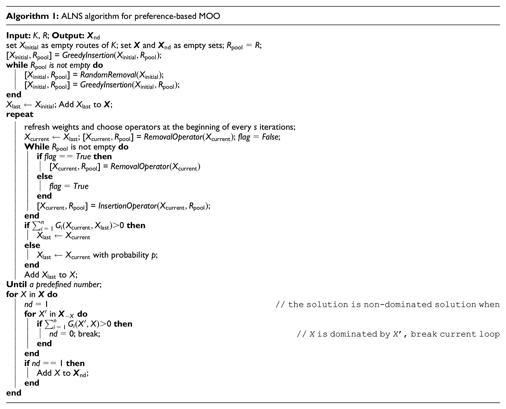
At the end of the iteration, a decision is made whether to accept current solution $X_{current}$ obtained in this iteration by comparing it with the last solution $X_{last}$ obtained in the last iteration. If the current solution is worse than the last solution, it will be accepted with a probability $p$ to avoid local optima more easily. Simulated annealing idea is used and probability $p$ gradually declines to avoid local optima ( 36 ), as the following equation shows:

p = e^{\frac{\sum_{i = 1}^{n} G_{i} (X_{current}, X_{last}) \cdot \sum_{n = 1}^{n} F_{i} (X_{current})}{T}},

(33)

where $T > 0$ is the temperature which starts from an initial temperature and gradually decreases in every iteration by cooling rate, $c$ , where $0 < c < 1$ . $n$ is the number of objectives and $F_{i} (X_{current})$ is the $i_{th}$ objective of $X_{current}$ . $\sum_{i = 1}^{n} G_{i} (X_{current}, X_{last})$ represents the dominance degree between $X_{current}$ and $X_{last}$ , which will be defined in Equation 38 when introducing the weight interval method.

After all solutions are obtained and stored in the solution set $X$ , $X_{nd}$ is obtained by comparing all solutions through the dominance rule. $X_{- X}$ means the solution set without $X$ .

The design of different operators is widely discussed in the literature ( 11 , 36 – 39 ) as well as the authors’ previous paper ( 12 ). Besides traditional operators, including Greedy Insertion, Transshipment Insertion, Random Insertion, Worst Removal, and Random Removal operators, this work designs two customized operators, that is, Route Removal and Node Removal operators. The following introduces the customized operators in detail and the others are introduced briefly.

Greedy Insertion operator tries all possible solutions using one vehicle and more than one vehicle and inserts the request into the best route(s) ( 38 , 39 ).

Transshipment Insertion operator also inserts requests greedily, but it only tries solutions using more than one vehicle and transshipment ( 11 , 39 ).

Random Insertion operator chooses vehicles and positions randomly and inserts the request once the solution is feasible ( 37 , 40 ).

Worst Removal operator removes the requests with the highest cost in each route ( 38 , 39 ).

Random Removal operator selects part of vehicles and removes one request from each vehicle randomly ( 37 , 40 ).

Route Removal: because of the interdependence of vehicles in ST, insertion operators may not be able to find feasible solutions based on a few removals in a short time. In this case, the route needs to be cleared, which means all requests in a route are removed to the request pool. Another idea behind this operator is to guide the search in the direction of minimizing the number of used vehicles and making full use of capacity. First, this operator obtains a random number $n$ with a given numerical distribution $[x_{1}, x_{2}, . . ., x_{3}]$ for $[1, 2, . . ., m]$ , where $m$ is the number of routes which served requests, $x_{1} = 1 / ξ$ and $x_{i} = x_{i - 1} / ξ$ when $i > 1$ . Then, it chooses $n$ vehicles according to a probability $ψ = u_{k}^{ava} / (\sum_{k \in K_{2 serve}} u_{k}^{ava})$ , where $u_{k}^{2 ava}$ is available capacity and $K_{serve}$ is a set of vehicles which have served requests. The vehicle whose capacity has not been fully made use of will have a higher probability of being cleared. In an extreme case, all routes will be cleared and all requests fill the request pool. In this case, this operator may change the search direction from the beginning and thus provide a larger neighborhood for insertion operators.

Node Removal: most of the time, barges and trains in ST carry multiple requests, therefore removing part of the requests may not change the routes of vehicles. However, the cost savings are usually obtained from minimizing distance, that is, changing the routes of vehicles. To obtain better solutions quicker, the Node Removal operator is designed, which deletes visited terminals from the routes. Similar to the Route Removal operator, this operator chooses $n$ vehicles based on a distribution and probability $ψ$ . One terminal of each route is randomly chosen and all requests which visit this terminal will be removed.

Synchronization Between Vehicles

This work studies the synchronization among vehicles, which means that vehicles can cooperate to get the best solution when a vehicle influences other vehicles (especially when there is transshipment between vehicles/modes). For example, in the transshipment terminal, if the delivery vehicle arrives later than the planned time, the route plan of the pickup vehicle needs to be synchronized to find a suitable arrival time. Synchronization is considered after ALNS operators are used. If the current solution violates constraints, such as time constraints, the synchronization procedure will start and make other vehicles cooperate with the insertion/removal. After the synchronization, the feasibility of the solution will be rechecked.

Four cases are listed below to illustrate the synchronization among vehicles in ST.

Synchronization Case 1

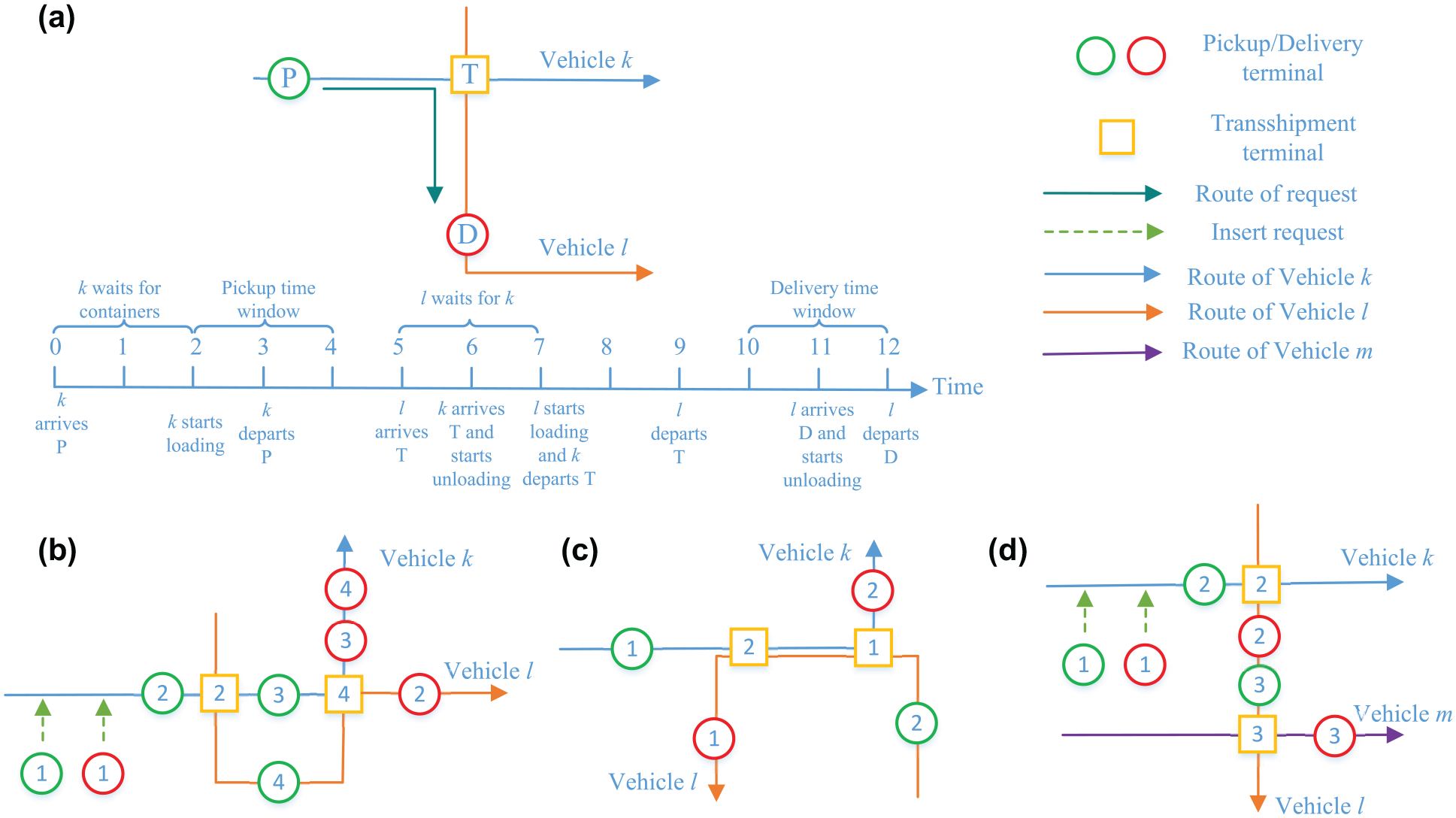
When a request is transported by more than one vehicle, the time between these vehicles is synchronized, as shown in Figure 3a. The time from the arrival time till the service start time is the waiting time, and departure happens after service time or transshipment time is completed. In Figure 3a, the request is first transported by vehicle $k$ and then transferred to vehicle $l$ . At the transshipment terminal, vehicle $k$ should arrive earlier than vehicle $l$ . However, vehicle $k$ arrives at transshipment terminal before vehicle $l$ completes the unloading, therefore vehicle $l$ waits for vehicle $k$ .

Figure 3.

Synchronization cases: (a) case 1: time synchronization in the transshipment terminal, (b) case 2: complex transshipment situation, (c) case 3: synchronization with cross requests, and (d) case 4: synchronization of relevant routes.

Synchronization Case 2

Extended from case 1, a more complex situation is considered, as shown in Figure 3b. When request 1 is inserted in vehicle $l$ , the pickup time of requests 3 and 4 will be influenced. If the waiting time for request 3 and 4 is changed, then the delivery time for requests 2, 3, and 4 need to be calculated based on both changes from insertion of request 1 and waiting time of request 3 and 4.

Synchronization Case 3

After the insertion, when there are cross requests, as shown in Figure 3c, the solution is infeasible. According to the time constraints, we have the following equations:

t_{Tp 2} < t_{Td 1},

(34a)

t_{Td 2} > t_{Tp 1},

(34b)

t_{Tp 2} > t_{Td 2},

(34c)

t_{Tp 1} > t_{Td 1},

(34d)

where $t_{Tp}$ means pickup time at transshipment terminal and $t_{Td}$ means delivery time at transshipment terminal. From Equation 34, we can get:

t_{Tp 1} > t_{Td 2},

(35)

which violates Equation 34b, therefore this solution is infeasible.

Synchronization Case 4

The synchronization for relevant vehicles is considered. Except for the situation described above, other vehicles may be influenced by the transshipment when one request is inserted or removed. As shown in Figure 3d, request 1 is inserted into the route of vehicle $l$ , and then vehicle $l$ is influenced by the transshipment of requests 2. Since the request 3 is transferred from vehicle $l$ to vehicle $m$ , the vehicle $m$ (such vehicles called relevant vehicles) is also influenced. In this research, these relevant vehicles can cooperate with changes by extending or shortening the waiting time.

Weight Interval Method

MOO aims to yield a set of non-dominated solutions presenting the optimal trade-offs between different objectives. These solutions are obtained by the Pareto improvement, which means a change to a different solution that makes at least one objective better off without making any other objective worse off. Figure 4 gives the Pareto frontier of bi-objective optimization for ST, where different DMs have different preferred solutions. As shown in Figure 4, preferred solutions are non-dominated solutions, which are in line with DMs’ preferences. DM A mainly wants to minimize the cost, DM C prefers to reduce the transport time, and DM B wants to balance cost and time. Based on their preferences, they will choose their preferred solutions in the Pareto frontier. Therefore, it is important to consider DMs’ preferences in MOO. Integrating preferences into the MOO approach and guiding the search toward solutions that are considered relevant by the DM may yield two important advantages:

Instead of a diverse set of solutions, many of them clearly irrelevant to the DM, a search guided toward the DM’s preferences will yield a more fine-grained and suitable selection of alternatives.

By focusing the search onto the relevant part of the search space, the objective space and the computation time can be reduced, especially when solving real-life MOO problems ( 20 , 41 ).

Using the weight interval method proposed by Szlapczynska and Szlapczynski ( 20 ), the vague preferences are added to ALNS. The weight interval which is assigned to the $i_{th}$ objective is:

w_{i} \in (w_{i}^{\min}, w_{i}^{\max}),

(36)

where $0 \leq w_{i}^{\min} < 1$ , $0 < w_{i}^{\max} \leq 1$ , and $w_{i}^{\min} \leq w_{i}^{\max}$ . The weight interval can represent vague preferences, such as linguistic terms.

Figure 4.

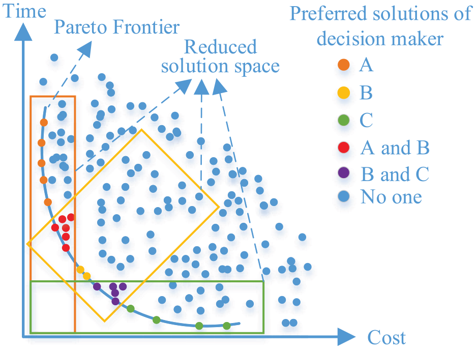
The Pareto frontier of bi-objective optimization for synchromodal transport.

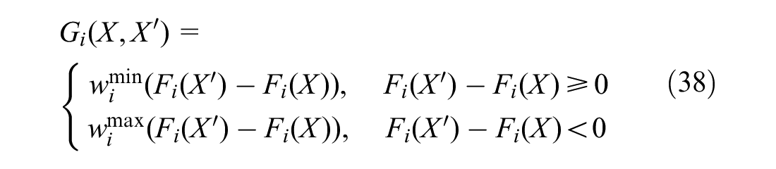
Under the vague preferences, the Pareto dominance rule is extended from traditional Pareto dominance ( 20 ). In this paper, solution $X$ dominates $X'$ when:

\sum_{i = 1}^{n} G_{i} (X, X') > 0,

(37)

where

\begin{matrix} G_{i} (X, X') = \\ {\begin{matrix} w_{i}^{\min} (F_{i} (X') - F_{i} (X)), & F_{i} (X') - F_{i} (X) \geq 0 \\ w_{i}^{\max} (F_{i} (X') - F_{i} (X)), & F_{i} (X') - F_{i} (X) < 0 \end{matrix} \end{matrix}

(38)

and $n$ is the number of objectives.

In ALNS, vague preferences are considered when comparing solutions. Before comparison, all objectives are normalized.

Case Study

The proposed model is applied to a ST network in the Rhine-Alpine corridor, which runs from Rotterdam to Genoa along the Rhine River through Europe’s industrial heart. All experiments are implemented in Python 3.7 and run with 8 GB of memory and an Intel Core i7 CPU with two 1.90 GHz and 2.11 GHz cores.

We assume that shippers provide the request information (including pickup and delivery terminals, number of containers, and time windows), and carriers provide transport network information (including terminal location and type, distances among terminals, vehicle information, and cost data). The coefficients, such as carbon emission, loading/unloading time, and transshipment cost, are derived from Van Riessen et al. ( 6 ), Guo et al. ( 34 ), and Li et al. ( 42 ). The coefficients used are as follows: $c_{k}^{1}$ / $c_{k}^{2}$ / $e_{k}$ equal to 0.2758/30.98/0.8866, 0.0213/0.6122/0.2288, and 0.0635/7.54/0.3146 for trucks, barges, and trains, respectively. $c_{k}^{3}$ / $c_{k}^{4}$ / $c_{k}^{5}$ / $c_{k}^{6}$ / ${t^{″}}_{i}^{k} / {t^{'″}}_{i}^{k}$ equal to 10/1/24/8/0.5/0.5, and they are the same for different modes. The parameter $ξ$ in Route Removal and Node Removal operators is set as 1.3 in this paper. The instances used are available at a research data website (https://figshare.com/s/4f7f513488accd5ecddb).

The parameters in ALNS need to be tuned before the optimization. To do that, the Pareto frontiers need to be compared in MOO instead of solutions comparison in the parameter tuning of single-objective optimization. The average value of all non-dominated solutions’ objective function values represent the Pareto frontier in the frontiers comparison, as Equation 39 shows:

P = \frac{\sum_{j = 1}^{m} \sum_{i = 1}^{n} F_{i} (X_{j})}{m},

(39)

where $P$ is the value which represents the Pareto frontier, $m$ is the number of non-dominated solutions, $n$ is the number of objectives, and $F_{i} (X_{j})$ is the $i_{th}$ normalized objective value of non-dominated solution $X_{j}$ . The parameters which generate minimum value $P$ will be used in the optimization.

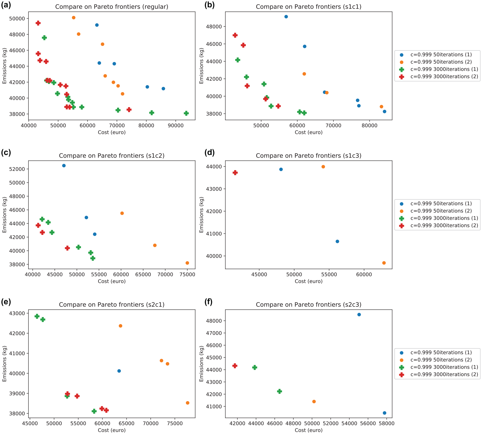
The parameters to be tuned include total iteration number, number of iterations for refreshing weights, initial temperature, and cooling rate. For example, the iteration number influences the quality of results, as shown in Figure 5, which shows Pareto frontiers for 10 requests and five vehicles under two objectives (cost and emission). Because $P_{3000 iterations}$ is less than $P_{50 iterations}$ , the Pareto frontiers with 3,000 iterations are better than frontiers with 50 iterations. It is worthy of note that these findings are only for this specific instance. Ideally, the parameters need to be tuned for each instance before the optimization.

Figure 5.

Pareto frontiers of bi-objective optimization under 50 iterations and 3,000 iterations: (a) regular Pareto frontier, (b) cost&emission: [0.1,0.9], (c) cost&emission: [0.25,0.75], (d) cost&emission: [0.33,0.66], (e) cost: [0.1,0.5], emission: [0.5,1.0], and (f) cost: [0.5,1.0], emission: [0.1,0.5].

The results for one of the experiments with five vehicles, 10 requests, and 10,000 iterations of ALNS are given in Figure 6. In this experiment, the objectives include cost and emissions. The requests and vehicles are randomly generated, and in total 19 terminals are used. The regular Pareto frontier, that is, Pareto frontier without preferences, is shown in Figure 6a. The other five figures compare the Pareto frontiers under different weight intervals with the regular Pareto frontier. Figure 6b to 6d, show the results when the weight interval narrows down from [0.1, 0.9] to [0.33, 0.66]. As the weight interval narrows down, the relative importance of cost and emissions is similar for both and therefore the trade-off between the objectives is more obvious. Figure 6e and 6f, show two opposite situations. In Figure 6e, the DM prefers to reduce emissions. In contrast, the DM favors reducing cost in Figure 6f.

Figure 6.

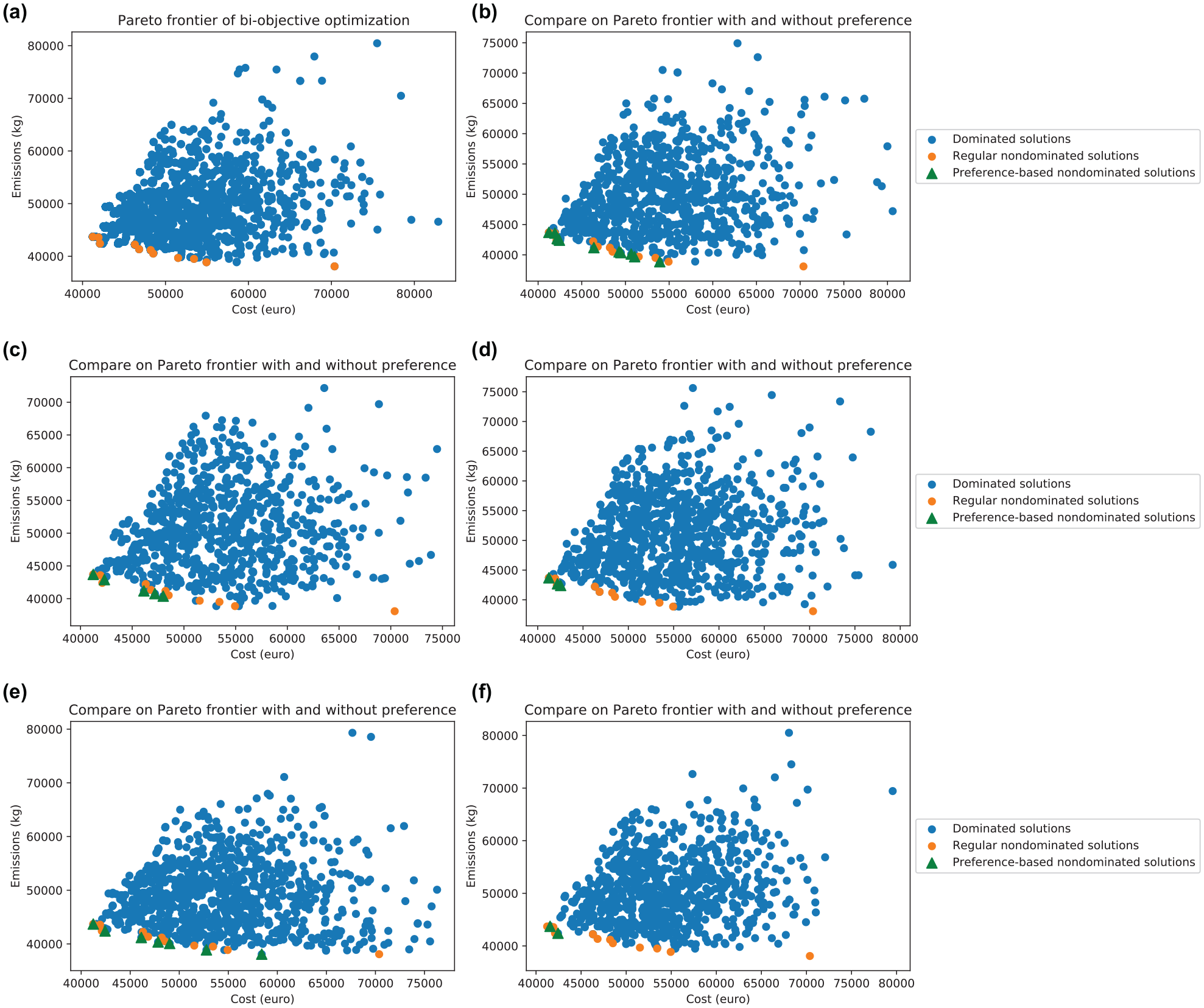
Pareto frontiers of bi-objective optimization: (a) regular Pareto frontier, (b) cost&emission: [0.1,0.9], (c) cost&emission: [0.25,0.75], (d) cost&emission: [0.33,0.66], (e) cost: [0.1,0.5], emission: [0.5,1.0], and (f) cost: [0.5,1.0], emission: [0.1,0.5].

It is interesting to investigate the following research question: What mode/route will the DMs with different preferences choose? To answer this research question, a case study is designed and five terminals are used, including two seaports (Rotterdam and Antwerp) and three inland terminals (Duisburg, Worth, and Basel). The transport network information is obtained from Contargo company (https://www.contargo.net/). Almost all modes can run between all terminals except for one situation: there is no train between Rotterdam and Antwerp. Table 3 shows the vehicle and request information. To guarantee that all modes have a similar chance to serve requests, different modes have the same number of vehicles, and there is no time window because vehicle speeds are different. Three objectives are considered: cost, emissions, and time.

Table 3.

Vehicle and Request Information

Vehicle	Capacity (TEU)	Speed (km/h)	Begin depot	Fixed route
Barge1	100	15	Antwerp	Free
Barge2	100	15	Rotterdam	Free
Truck1	50	75	Antwerp	Free
Truck2	50	75	Rotterdam	Free
Train1	75	45	Antwerp	Antwerp-Duisburg-Worth-Basel
Train2	75	45	Rotterdam	Rotterdam-Duisburg-Worth-Basel
Request	Pickup terminal	Delivery terminal	Time window	Load
0	Antwerp	Duisburg	Free	25
1	Rotterdam	Duisburg	Free	50
2	Antwerp	Worth	Free	25
3	Rotterdam	Worth	Free	50
4	Antwerp	Basel	Free	25
5	Rotterdam	Basel	Free	50
6	Duisburg	Worth	Free	25
7	Duisburg	Basel	Free	50
8	Worth	Basel	Free	25
9	Antwerp	Rotterdam	Free	50

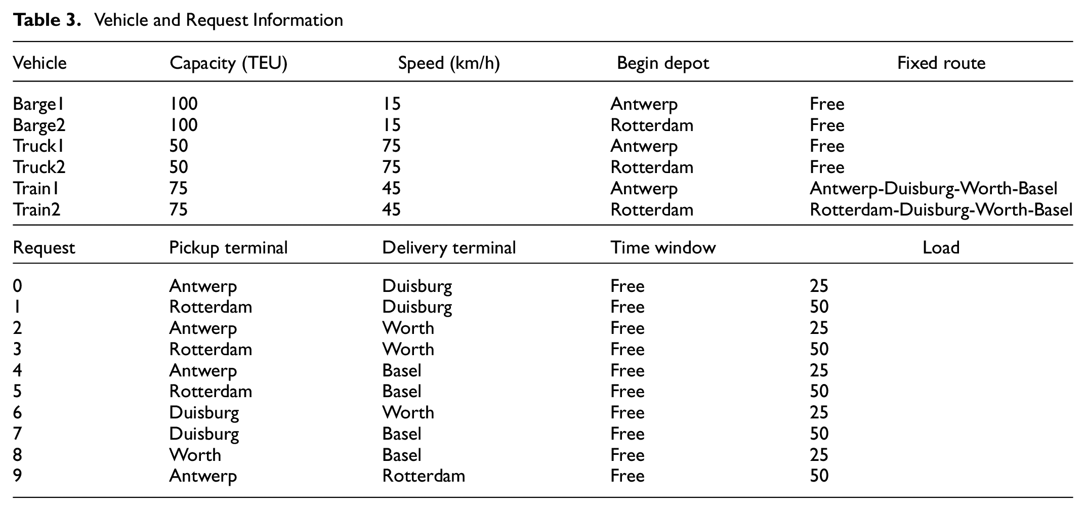
In this case, 10 instances are generated from 10 requests, that is, the ith instance includes $i$ request(s). For example, the fifth instance includes requests 0–4. The upper part of Table 4 shows regular (meaning no preferences) non-dominated solutions with request 1. Except for Truck1 in Solution 5, which is empty from Antwerp to Rotterdam, other vehicles transport request 1 on their routes. Solution 1 is also the best solution for cost minimization (single-objective optimization) and the barge is used in this solution. From these non-dominated solutions, we can see that different modes and routes are used after emission and time objectives are considered. This insight is useful to see the impact of different policies on transportation networks with regard to environmental considerations.

Table 4.

Regular Non-Dominated Solutions and Mode Shares of Different Cases

Solution	Cost (euro)	Time (h)	Emission (kg)	Vehicles and routes
1	4379.309	27.16	2158.728	Barge1: Antwerp → Duisburg
2	5979.755	10.387	2968.251	Train1: Antwerp → Duisburg
3	6756.684	15.831	2753.751	Barge1: Antwerp → Rotterdam;
				Train2: Rotterdam → Duisburg
4	6004.381	23.716	2373.228	Train1: Antwerp → Rotterdam;
				Barge2: Rotterdam → Duisburg
5	11394.345	10.254	6935.071	Truck1: Antwerp → Rotterdam → Duisburg;
				Train1: Antwerp → Rotterdam
6	10351.813	7.032	8365.071	Truck1: Antwerp → Duisburg
Name	Average cost (euro)	Average emission (kg)	Average time (h)	Share of barge (%)	Share of train (%)	Share of truck (%)
Regular	35710.5	31635.6	95.2	49.87	39.58	10.55
s1c1	30283.7	28549.2	96.0	64.93	33.97	1.1
s1c2	29628.0	28367.4	94.4	62.08	37.40	0.53
s1c3	27546.1	27457.4	98.6	73.37	26.16	0.48
s2c1	26966.5	27195.0	100.8	72.14	27.86	0
s2c2	28306.0	27068.6	103.0	72.13	27.39	0.48
s2c3	33250.9	30068.9	85.7	42.57	54.75	2.68
Average	30241.7	28620.3	96.3	62.44	35.30	2.26

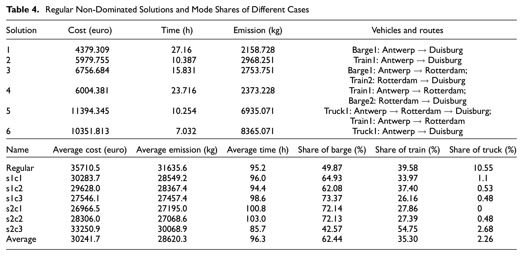
Besides the regular case, two scenarios (each scenario includes three cases) with preferences are designed. The weight intervals of three objectives in the first scenario are the same but narrow down from case s1c1 (meaning scenario 1 case 1) to s1c3. The weight intervals of s1c1, s1c2, and s1c3 are [0.1,0.9], [0.25,0.75], and [0.33,0.66], respectively. In the second scenario, each case prefers one objective. Cases s2c1, s2c2, and s2c3 prefer minimizing cost, emissions, and time, respectively. The weight interval of the preferred objective is [0.5,1.0], and weight intervals of the other two objectives are [0.1,0.5]. For example, the weight intervals of s2c1 are Cost: [0.5,1.0], Emission&Time: [0.1,0.5].

For each instance, there are seven cases and each case is repeated three times to obtain the average value. Therefore, a total of 210 experiments were performed. In each experiment, ALNS runs for 1,000 iterations and the computation time depends on instance size. For the instances with one request and 10 requests, the computation times are around 1 min and 15 min, respectively. The share of used modes is calculated for every case, as shown in the bottom part of Table 4. The results show that the solution tends to be better when the weight narrows down in the first scenario (s1c1, s1c2, and s1c3) as the cost, emissions, and time reduce. The share of the barge in s1c3 is larger than in s1c2 because s1c3 sacrifices time in exchange for better cost and emission, thus making the overall result better. In the second scenario, the minimum value of each objective is in line with preferences. The parameters used in this paper set the barge as having the lowest cost, emissions, and speed, and the truck is the fastest but has the highest cost and emissions. Therefore, the barge is used the most when costs or emissions are prioritized. Nevertheless, when time is minimized (s2c3) the train’s share becomes the highest because the barge speed is too low and truck’s cost and emissions are high. The results are sensitive to the cost, emissions, and time parameters. When the parameters change in reality, the share of modes may also change. In inland waterway transport, there are more uncertainties than other modes, such as long waiting times, lock/bridge open time, and changing water level. In the meantime, compared with other modes, there may be limited depth and inadequate air draft in inland waterway transport. Therefore, although the results in this paper show the advantages of barges and encourage DMs to choose barges, barges are not utilized as frequently in reality. The uncertainties and limitations of modes will be considered in the future to make the model more practical.

The proposed model is also compared with a recent paper ( 34 ), using the same instances. Guo et al. ( 34 ) solved a similar ST planning problem with us and minimized the transport cost, but they did not consider preferences. Guo et al. ( 34 )’s instances are based on a transport network operated by European Gateway Services, which contains 116 vehicles (49 barges, 33 trains, and 34 trucks) and 10 terminals (three deep-sea terminals and seven inland terminals, and all terminals could be used as transshipment terminals). In the following results, the same cost objective is used as in Guo et al. ( 34 ). Table 5 shows the results of instances with five, 10, 20, and 30 requests under two conflicting objectives, that is, minimizing cost and time. Under the same setting, the proposed model can find the same solution as Guo et al. ( 34 ), and the results are not repeated in Table 5. In instances with five and 10 requests, the transport cost is the same as in Guo et al. ( 34 ) when the DM prefers the cost objective because the latter solution dominates other solutions. In instances with 20 and 30 requests, the transport cost is slightly higher than in Guo et al. ( 34 ) and the transport time decreases because the transport time of that solution cannot satisfy the preferences on both cost and time objectives. When the DM prefers the Time objective, the transport time is reduced more, and the mode shares of trains and trucks increase. This comparison shows that the proposed methodology finds the optimal solutions when the objective is the same and that the solutions can be adapted to the preferences of the carrier with a multi-objective setting with preferences.

Table 5.

Comparison with Guo et al. ( 34 )

Number of requests	Average cost (euro)	Average time (h)	Share of barge (%)	Share of train (%)	Share of truck (%)
5 ☆	4386	29	60	0	40
5 ○	4386	29	60	0	40
5 ◇	4386	29	60	0	40
10 ☆	25988	151	50	29	21
10 ○	25988	151	50	29	21
10 ◇	36351	127	47	28	25
20 ◇	44198	236	57	18	25
20 ○	44858	212	54	19	27
20 ◇	58787	163	52	26	22
30 ☆	65126	329	50	11	39
30 ○	69824	326	49	12	39
30 ◇	85484	271	48	11	41

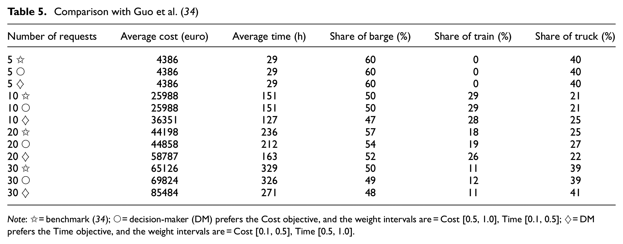
Note: ☆ = benchmark ( 34 ); ○ = decision-maker (DM) prefers the Cost objective, and the weight intervals are = Cost [0.5, 1.0], Time [0.1, 0.5]; ◇ = DM prefers the Time objective, and the weight intervals are = Cost [0.1, 0.5], Time [0.5, 1.0].

Conclusion and Future Studies

In this research, a preference-based MOO (PMOO) model is developed to address the conflicts among multiple objectives of carriers in ST. Compared with models in the literature ( 3 , 28 , 30 ), the contributions of this work are the considerations of vehicle routing, synchronization, and preferences in ST. The VRP is regarded as a PDPT, and both vehicle routing and container flow are modeled to achieve the transshipment in ST. Because of the requirements of ST, the synchronization between vehicles is considered, which makes the model more flexible. Based on the optimization model, which considers vehicle routing and synchronization, the weight interval is incorporated into ALNS to represent the vague preferences of DMs. The case study on the Rhine-Alpine corridor verified that the proposed model provides non-dominated solutions which reveal DM preferences. Under different preferences in this paper, the barge is the most popular transport mode because of its low cost and low emissions. When a DM prefers to minimize transport time, transport modes with higher speed are used more frequently. It is worth noticing that the mode used is dependent on the input parameters. When these parameters change in another instance, the mode share may be different.

The proposed model is able to target a selected part of the Pareto frontier based on a DM’s vague preferences. This is a significant advantage for carriers in ST because they can just enter their linguistic preferences and then obtain solutions which reveal their preferences. Using the proposed model, DMs do not need to struggle to solve conflicts between their objectives from many solutions with different modes and routes. Compared with MOO without preferences, this model not only reduces the number of alternatives but also chooses solutions which are preferred by DMs.

The proposed model can be encapsulated in a software application in the intermodal transport domain. DMs enter transport network information, requests, and preferences into the software and then they will obtain preferred solutions. The model is designed for intermodal container transport, but it can also be applied to other transport domains if the shipments are non-splittable, such as truck-load transport. Moreover, this work combined PMOO and PDPT in ST, which may be helpful for solving similar problems in the VRP domain.

Future research will focus on the following aspects:

A carrier usually transports containers for multiple shippers with heterogeneous preferences, such as low-cost, fast, sustainable, reliable, or low-risk transport. To improve the service quality and gain superiority in the business competition, the carrier needs to satisfy the expectations of shippers. Therefore, future research will study ST planning considering the heterogeneous preferences of shippers.

Collaborative planning among carriers is an interesting direction, which may reduce transport cost, time, and emissions. Shippers can also identify attractive bundles of requests and consolidate their cargo to help the carriers in reducing empty trips and making full use of the capacity of the vehicles ( 43 ). Conflicts between preferences also happen in collaborative planning among carriers and shippers. Therefore, the PMOO model for collaborative planning is a promising research direction.

Uncertainties are common in ST, such as delay (travel time uncertainty) and new requests from a spot market (demand uncertainty). Considering uncertainties in the proposed model is also an interesting direction. The current model assumes that all vehicles are available at their begin depot from time 0. In reality, vehicles are not always available because of travel time uncertainties, such as delay and bad weather. Therefore, an interesting future research direction is the incorporation of uncertainties both on the availability of the services and also on the demand side. For example, if serving a new request can make the DM more satisfied, the original plan can be changed.

Footnotes

Author Contributions

The authors confirm contribution to the paper as follows: study conception and design: Y. Zhang, B. Atasoy, R. R. Negenborn; data collection: Y. Zhang; analysis and interpretation of results: Y. Zhang, B. Atasoy; draft manuscript preparation: Y. Zhang, B. Atasoy. All authors reviewed the results and approved the final version of the manuscript.

Declaration of Conflicting Interests

The author(s) declared no potential conflicts of interest with respect to the research, authorship, and/or publication of this article.

Funding

The author(s) disclosed receipt of the following financial support for the research, authorship, and/or publication of this article: This research is supported by the China Scholarship Council under Grant 201906950085 and the project “Complexity Methods for Predictive Synchromodality” (project 439.16.120) of the Netherlands Organization for Scientific Research (NWO). This research is also supported by the project “Novel inland waterway transport concepts for moving freight effectively (NOVIMOVE)”. This project has received funding from the European Union’s Horizon 2020 research and innovation program under grant agreement No 858508.

ORCID iDs

Yimeng Zhang

Bilge Atasoy

Rudy R. Negenborn

References

SteadieSeifi

Dellaert

N. P.

Nuijten

Van Woensel

Raoufi

Multimodal Freight Transportation Planning: A Literature Review. European Journal of Operational Research, Vol. 233, No. 1, 2014, pp. 1–15.

Sun

S. X.

Dai

Intermodal Transportation Service Procurement with Transaction Costs Under Belt and Road Initiative. Transportation Research Part E: Logistics and Transportation Review, Vol. 127, 2019, pp. 31–48.

Kalinina

Olsson

Larsson

A Multi Objective Chance Constrained Programming Model for Intermodal Logistics with Uncertain Time. International Journal of Computer Science Issues, Vol. 10, No. 6, 2013, pp. 35–44.

Ambra

Caris

Macharis

Towards Freight Transport System Unification: Reviewing and Combining the Advancements in the Physical Internet and Synchromodal Transport Research. International Journal of Production Research, Vol. 57, No. 6, 2019, pp. 1606–1623.

Giusti

Manerba

Bruno

Tadei

Synchromodal Logistics: An Overview of Critical Success Factors, Enabling Technologies, and Open Research Issues. Transportation Research Part E: Logistics and Transportation Review, Vol. 129, 2019, pp. 92–110.

Van Riessen

Negenborn

R. R.

Dekker

Lodewijks

Service Network Design for an Intermodal Container Network with Fexible Transit Times and the Possibility of Using Subcontracted Transport. International Journal of Shipping and Transport Logistics, Vol. 7, No. 4, 2015, pp. 457–478.

Zhu

Crainic

T. G.

Gendreau

Scheduled Service Network Design for Freight Rail Transportation. Operations Research, Vol. 62, No. 2, 2014, pp. 383–400.

Drexl

Synchronization in Vehicle Routing: A Survey of VRPs with Multiple Synchronization Constraints. Transportation Science, Vol. 46, No. 3, 2012, pp. 297–316.

Drexl

Branch-and-Cut Algorithms for the Vehicle Routing Problem with Trailers and Transshipments. Networks, Vol. 63, No. 1, 2014, pp. 119–133.

10.

Grangier

Gendreau

Lehuédé

Rousseau

L.-M.

A Matheuristic Based on Large Neighborhood Search for the Vehicle Routing Problem with Cross-Docking. Computers & Operations Research, Vol. 84, 2017, pp. 116–126.

11.

Masson

Lehuédé

Péton

An Adaptive Large Neighborhood Search for the Pickup and Delivery Problem with Transfers. Transportation Science, Vol. 47, No. 3, 2013, pp. 344–355.

12.

Zhang

Atasoy

Souravlias

Negenborn

R. R.

Pickup and Delivery Problem with Transshipment for Inland Waterway Transport. In Proc., 11th International Conference on Computational Logistics ( Lalla-Ruiz

Mes

Voß

, eds.), Enschede, The Netherlands, September 28–30, 2020, Springer, Cham, pp. 18–35.

13.

Behdani

Fan

Wiegmans

Zuidwijk

Multimodal Schedule Design for Synchromodal Freight Transport Systems. European Journal of Transport and Infrastructure Research, Vol. 16, No. 3, 2014, pp. 424–444.

14.

Sarasola

Doerner

K. F.

Adaptive Large Neighborhood Search for the Vehicle Routing Problem with Synchronization Constraints at the Delivery Location. Networks, Vol. 75, No. 1, 2020, pp. 64–85.

15.

Masson

Lehuédé

Péton

The Dial-a-Ride Problem with Transfers. Computers & Operations Research, Vol. 41, 2014, pp. 12–23.

16.

Grangier

Gendreau

Lehuédé

Rousseau

L.-M.

An Adaptive Large Neighborhood Search for the Two-Echelon Multiple-Trip Vehicle Routing Problem with Satellite Synchronization. European Journal of Operational Research, Vol. 254, No. 1, 2016, pp. 80–91.

17.

Drexl

Applications of the Vehicle Routing Problem with Trailers and Transshipments. European Journal of Operational Research, Vol. 227, No. 2, 2013, pp. 275–283.

18.

Wang

Olhofer

Jin

A Mini-Review on Preference Modeling and Articulation in Multi-Objective Optimization: Current Status and Challenges. Complex & Intelligent Systems, Vol. 3, No. 4, 2017, pp. 233–245.

19.

Coello

C. A. C.

Lamont

G. B.

Van Veldhuizen

D. A.

Evolutionary Algorithms for Solving Multi-Objective Problems, Springer, Boston, MA, 2007.

20.

Szlapczynska

Szlapczynski

Preference-Based Evolutionary Multi-Objective Optimization in Ship Weather Routing. Applied Soft Computing, Vol. 84, 2019, p. 105742.

21.

Liu

H.-L.

Integrating Preference by Means of Desirability Function with Evolutionary Multi-Objective Optimization. Intelligent Automation & Soft Computing, Vol. 21, No. 2, 2015, pp. 197–209.

22.

Gören

Baccouche

Pierreval

A Framework to Incorporate Decision-Maker Preferences into Simulation Optimization to Support Collaborative Design. IEEE Transactions on Systems, Man, and Cybernetics: Systems, Vol. 47, No. 2, 2016, pp. 229–237.

23.

Battiti

Passerini

Brain–Computer Evolutionary Multiobjective Optimization: A Genetic Algorithm Adapting to the Decision Maker. IEEE Transactions on Evolutionary Computation, Vol. 14, No. 5, 2010, pp. 671–687.

24.

Ghodsi

S. H.

Kerachian

Zahmatkesh

A Multi-Stakeholder Framework for Urban Runoff Quality Management: Application of Social Choice and Bargaining Techniques. Science of the Total Environment, Vol. 550, 2016, pp. 574–585.

25.

Deb

Pratap

Agarwal

Meyarivan

A Fast and Elitist Multiobjective Genetic Algorithm: NSGA-II. IEEE Transactions on Evolutionary Computation, Vol. 6, No. 2, 2002, pp. 182–197.

26.

Xiong

Wang

Best Routes Selection in Multimodal Networks Using Multi-Objective Genetic Algorithm. Journal of Combinatorial Optimization, Vol. 28, No. 3, 2014, pp. 655–673.

27.

Baykasoğlu

Subulan

A Multi-Objective Sustainable Load Planning Model for Intermodal Transportation Networks with a Real-Life Application. Transportation Research Part E: Logistics and Transportation Review, Vol. 95, 2016, pp. 207–247.

28.

Luo

A Hybrid Estimation of Distribution Algorithm for Multi-Objective Multi-Sourcing Intermodal Transportation Network Design Problem Considering Carbon Emissions. Sustainability, Vol. 9, No. 7, 2017, p. 1133.

29.

Mnif

Bouamama

Firework Algorithm for Multi-Objective Optimization of a Multimodal Transportation Network Problem. Procedia Computer Science, Vol. 112, 2017, pp. 1670–1682.

30.

Chen

Zhang

Gao

Thompson

R. G.

Optimizing Multimodal Transportation Routes Considering Container Use. Sustainability, Vol. 11, No. 19, 2019, p. 5320.

31.

Waltho

Elhedhli

Gzara

Green Supply Chain Network Design: A Review Focused on Policy Adoption and Emission Quantification. International Journal of Production Economics, Vol. 208, 2019, pp. 305–318.

32.

Demir

Burgholzer

Hrušovský

Arıkan

Jammernegg

Van Woensel

A Green Intermodal Service Network Design Problem with Travel Time Uncertainty. Transportation Research Part B: Methodological, Vol. 93, 2016, pp. 789–807.

33.

Huang

Wen

Zhang

Zhou

Zhang

Yang

Dynamic Calculation of Ship Exhaust Emissions Based on Real-Time AIS Data. Transportation Research Part D: Transport and Environment, Vol. 80, 2020, p. 102277.

34.

Guo

Atasoy

Beelaerts van Blokland

W. W. A.

Negenborn

R. R.

A Dynamic Shipment Matching Problem in Hinterland Synchromodal Transportation. Decision Support Systems, Vol. 134, 2020, p. 113289.

35.

Öncan

Altınel

I. K.

Laporte

A Comparative Analysis of Several Asymmetric Traveling Salesman Problem Formulations. Computers & Operations Research, Vol. 36, No. 3, 2009, pp. 637–654.

36.

Ropke

Pisinger

An Adaptive Large Neighborhood Search Heuristic for the Pickup and Delivery Problem with Time Windows. Transportation Science, Vol. 40, No. 4, 2006, pp. 455–472.

37.

Bard

J. F.

A GRASP with Adaptive Large Neighborhood Search for Pickup and Delivery Problems with Transshipment. Computers & Operations Research, Vol. 39, No. 10, 2012, pp. 2439–2456.

38.

Ghilas

Demir

Van Woensel

An Adaptive Large Neighborhood Search Heuristic for the Pickup and Delivery Problem with Time Windows and Scheduled Lines. Computers & Operations Research, Vol. 72, 2016, pp. 12–30.

39.

Wolfinger

A Large Neighborhood Search for the Pickup and Delivery Problem with Time Windows, Split Loads and Transshipments. Computers & Operations Research, Vol. 126, 2021, p. 105110.

40.

Danloup

Allaoui

Goncalves

A Comparison of Two Meta-Heuristics for the Pickup and Delivery Problem with Transshipment. Computers & Operations Research, Vol. 100, 2018, pp. 155–171.

41.

Branke

Deb

Integrating User Preferences into Evolutionary Multi-Objective Optimization. In Knowledge Incorporation in Evolutionary Computation ( Yaochu

, ed.), Springer, Berlin, Heidelberg, 2005, pp. 461–477.

42.

Negenborn

R. R.

Lodewijks

Distributed Constraint Optimization for Addressing Vessel Rotation Planning Problems. Engineering Applications of Artificial Intelligence, Vol. 48, 2016, pp. 159–172.

43.

Chabot

Bouchard

Legault-Michaud

Renaud

Coelho

L. C.

Service Level, Cost and Environmental Optimization of Collaborative Transportation. Transportation Research Part E: Logistics and Transportation Review, Vol. 110, 2018, pp. 1–14.

Preference-Based Multi-Objective Optimization for Synchromodal Transport Using Adaptive Large Neighborhood Search

Abstract

Keywords

Literature Review

Transshipment

Synchronization

Preference-Based Multi-Objective Optimization

MOO for Intermodal Transport

Problem Description

Mathematical Model

Solution Methodology

ALNS Algorithm

Synchronization Between Vehicles

Synchronization Case 1

Synchronization Case 2

Synchronization Case 3

Synchronization Case 4

Weight Interval Method

Case Study

Conclusion and Future Studies

Footnotes

Author Contributions

Declaration of Conflicting Interests

Funding

ORCID iDs

References