Sage Journals: Discover world-class research

Abstract

Objective

The automatic detection of migraine states using electrophysiological recordings may play a key role in migraine diagnosis and early treatment. Migraineurs are characterized by a deficit of habituation in cortical information processing, causing abnormal changes of somatosensory evoked potentials. Here, we propose a machine learning approach to utilize somatosensory evoked potential-based biomarkers for migraine classification in a noninvasive setting.

Methods

Forty-two migraine patients, including 29 interictal and 13 ictal, were recruited and compared with 15 healthy volunteers of similar age and gender distribution. The right median nerve somatosensory evoked potentials were collected from all subjects. State-of-the-art machine learning algorithms including random forest, extreme gradient-boosting trees, support vector machines, K-nearest neighbors, multilayer perceptron, linear discriminant analysis, and logistic regression were used for classification and were built upon somatosensory evoked potential features in time and frequency domains. A feature selection method was employed to assess the contribution of features and compare it with previous clinical findings, and to build an optimal feature set by removing redundant features.

Results

Using a set of relevant features and different machine learning models, accuracies ranging from 51.2% to 72.4% were achieved for the healthy volunteers-ictal-interictal classification task. Following model and feature selection, we successfully separated the three groups of subjects with an accuracy of 89.7% for the healthy volunteers-ictal, 88.7% for healthy volunteers-interictal, 80.2% for ictal-interictal, and 73.3% for healthy volunteers-ictal-interictal classification tasks, respectively.

Conclusion

Our proposed model suggests the potential use of somatosensory evoked potentials as a prominent and reliable signal in migraine classification. This non-invasive somatosensory evoked potential-based classification system offers the potential to reliably separate migraine patients in ictal and interictal states from healthy controls.

Keywords

Migraine attack electrophysiological recording machine learning feature selection early detection

Introduction

Migraine is a disabling neurological disorder, characterized by recurrent headache attacks. Despite its high prevalence, migraine diagnosis is still mainly based on clinical interviews, patient diaries, and physical examinations. More advanced diagnostic methods are therefore desired for both clinical and research purposes and can potentially aid in early diagnosis and assessment of disease progression. Given the lack of consistent structural abnormalities, clinical neurophysiology methods are particularly suited to study the pathophysiology of migraine (1). The neurophysiological techniques have been recently used in assessing the clinical fluctuations in migraine (2), and the effectiveness of emerging neuromodulation therapies such as repetitive transcranial magnetic stimulation (3). Considering that early treatment of migraine headache is shown to be significantly more effective (4), it is important to predict migraine early in the course of attack, potentially with automated monitoring techniques. While wearable sensors and medical devices are increasingly being applied to the early diagnosis and treatment of neurological disorders, the field is relatively unexplored in migraine treatment. Such devices can detect the neurological abnormalities in real time and prompt patients to take preventive medications, monitor the progression of disease and effectiveness of medications, or trigger a therapy such as neuromodulation (5,6). Given the potential of noninvasive electrophysiological techniques recently shown in clinical migraine studies (2,7,8), particularly the somatosensory evoked cortical potentials, we aim at assessing their power in classifying various states of migraine and separating migraine patients from healthy controls. This approach could potentially be used for early diagnosis of migraine attacks in a wearable setting in future.

According to most electrophysiological studies, migraine patients are characterized by hyper-responsivity in both somatosensory and visual cortices (9), which can be measured by standard electrophysiological techniques such as somatosensory evoked potential (SSEP) and visual evoked potential (VEP). Given the ease of evoking SSEPs (e.g. using a wristband-type device), our approach is based on the former. The SSEP correlates of the migraine brain were first reported in 2005 (7). In particular, a lack of habituation in response to repetitive stimuli was found in migraine patients in the interictal state, both with (MA) or without aura (MO). The high-frequency oscillations (HFOs) superimposed on the median nerve SSEPs are widely reported as indicators of thalamo-cortical activation (10). More specifically, the early and late HFO bursts are thought to be generated by the thalamo-cortical afferents and inhibitory neurons in the parietal cortex, respectively. A reduction of early HFO between attacks and increase of late HFO during attacks have been previously reported in migraine patients (8,9). In addition to HFOs, some low-frequency components are also critical in characterizing various states of migraine. For instance, the increased N20-P25 amplitude of low-frequency SSEP has been associated with the migraine ictal group (8). Based on the altered SSEP signals in migraine patients, the associated HFO and low-frequency components could be used as potential features for our classification task. In other words, despite many unknowns in pathogenesis and underlying causes of migraine, the associated changes of SSEPs allow us to reliably differentiate between the ictal or interictal phases of migraine, as well as healthy controls.

Although the electroencephalogram (EEG)-based biomarkers have been widely used in other neurological fields of research, such as epilepsy (11), studies on SSEP features are very limited. The resting-state EEG complexity was recently shown to be higher in the migraine preictal compared to the interictal group. The variations of EEG complexity were subsequently used to classify the preictal and interictal states of migraine (12). In addition to complexity, other relevant biomarkers such as spectral power in different frequency bands and time-domain variance of EEG were extracted and tested using various machine learning models, such as support vector machines and neural networks (13,14). However, the EEG-based classification systems generally require multiple channels, which may add to the complexity of data acquisition and processing. Functional magnetic resonance imaging (fMRI) is another effective tool for migraine analysis, which was further used for classification of migraine from healthy controls (15). However, fMRI and other neuroimaging techniques are costly and cumbersome for routine use and are currently impossible to integrate into portable devices. The limited temporal resolution of fMRI and computational overhead of image classification are the other drawbacks of this approach.

Alternatively, we propose to employ SSEP as a practical diagnostic tool and a sensitive predictor for migraine classification. Our goal is to distinguish migraine patients in different phases (interictal or ictal) from healthy controls, using state-of-the-art machine learning models and SSEP biomarkers. The proposed system was trained and validated on a dataset of 57 subjects. We further analyzed the most discriminating features for each classification task. This approach is the first step toward early detection of migraine attacks, which could be used in a personalized headache monitoring device.

Materials and methods

The block diagram of the proposed migraine classification system is shown in Figure 1. The SSEP signals were recorded from healthy subjects and from migraineurs in the two phases of ictal and interictal. The raw signals are plotted as time series and their time-frequency distributions are further analyzed to find the dominant high-frequency components. From the time-frequency graph, we were able to identify two peaks in the high frequency range, which were later defined as early and late HFOs. We performed preprocessing on the raw data by removing artifacts and averaging over multiple SSEP trials. Several biomarkers were then extracted using Fourier transform and digital filtering. The evaluated feature set is composed of spectral power in different frequency bands, low-frequency (LF) features, and HFO-related biomarkers. A wrapper-based feature selection method was used to select the most discriminative features. Several machine learning models were then tested on the resulting feature set and their parameters were carefully optimized. Finally, we compared the classifier outputs with the actual labels to calculate the prediction accuracy.

Figure 1.

Block diagram of the proposed migraine state classification system. The SSEP signals were recorded using a CED 1401 device with electrical stimulation applied to the wrist. After artifact removal and averaging, migraine features were extracted in both time and frequency domains. A feature selection approach was employed to find the optimal feature set for each task. Various models and classifiers were further tested and optimized to achieve the best classification results.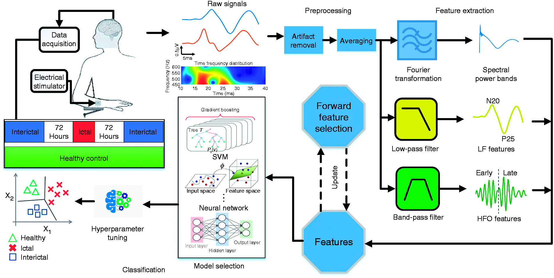

Participants

We initially enrolled 50 consecutive migraine patients who attended our headache clinic. Of the patients initially recorded, eight patients had an attack between 12 and 72 hours before or after the recording session, and their electrophysiological data were not included in the subsequent analysis. The final data set comprises a total number of 42 migraine patients, including 29 interictal (15 MA, 14 MO, 17 females, 12 males) and 13 ictal (four MA, nine MO, 11 females, two males). The subjects were recruited among the patients attending the headache clinic of Sapienza University of Rome and the demographic characteristics of the migraine patients are included in Supplemental Table 1. We excluded those patients who had taken medication regularly, except for the contraceptive pill. For comparison, we enrolled a group of 15 age-matched healthy volunteers recruited among medical school students and healthcare professionals. The patients and controls were examined at the same time of day, in the same laboratory and by the same investigators. Patients in the interictal state were recorded at least 72 hours before or after a migraine attack. The ictal group consisted of patients who had an interval of less than 12 hours between the recording time and a migraine attack. The study was approved by the Ethics Committee of the Faculty of Medicine, University of Rome. Informed consent was collected from all participants in this study.

Data acquisition

The SSEP signals were elicited by electrical stimulation of the median nerve and recorded using a CED 1401 device (Cambridge Electronic Design Ltd, Cambridge, UK). Subjects were asked to sit comfortably on a chair in an illuminated room and keep their eyes open, with their attention focused on the wrist movement. Electrical stimulation was applied to the right median nerve at the wrist with a constant-current square-wave pulse (0.2 ms width, cathode proximal). The stimulus intensity was set at twice the motor threshold with a repetition rate of 4.4 Hz. The SSEP signals were recorded over the contralateral parietal area. The ground electrode was placed on the right arm. A CED™ 1902 was used to amplify the evoked potentials. The sampling frequency was set to 5000 Hz and the post-stimulus signals were recorded for a duration of 40 ms. The high sampling rate allowed us to analyze a wide range of frequency bands in the subsequent feature extraction stage.

Data analysis and feature extraction

The SSEP signals were low-pass filtered at 450 Hz to extract the low-frequency (LF) components. The LF-SSEPs were then used to identify the latency of various SSEP components (N20, P25) and the associated peak-to-peak amplitude.

Prior studies have shown that high-frequency oscillations (HFOs) embedded on the parietal N20 component of SSEPs are significantly different in migraineurs between attacks, compared to healthy volunteers (7,17 –20). This indicates that HFO could be an important biomarker to distinguish migraineurs from healthy subjects. Here, we extracted HFOs using an FIR bandpass filter (450–750 Hz). Both low-pass and band-pass filters were designed using a Bartlett-Hanning window with a filter order of 50. Between the early and late HFO bursts, a clear change in both frequency and amplitude was observed in the majority of recordings. More specifically, the early burst was in the ascending slope of the N20 component, while the late burst occurred in the descending slope of N20, sometimes extending toward the ascending slope of N33 (8). The N20 peak latency was used as a cut-off point to separate early and late HFO bursts (27), while both HFOs had an approximate duration of 5 ms (20).

Figure 2(a) illustrates the average SSEP recordings of individuals from each group, while Figure 2(b) shows the low-frequency SSEPs and the embedded high-frequency oscillations. The N20-P25 amplitudes of LF-SSEPs were found to be larger in the ictal group. The maximum peak-to-peak amplitude of the late HFO burst was different between the HV and MI groups, while MO and MA tended to be lower in the early HFOs. Considering the lack of significant difference in the HFO or LF components between the MO and MA groups, we combined them into one interictal class for the subsequent feature extraction and classification process.

Figure 2.

(a) Grand averaged SSEP recordings from migraine patients as well as healthy controls; (b) the amplitude changes in the N20-P25 peak-to-peak value of averaged SSEPs and the extracted HFOs from all groups; (c) statistical analysis of N20-P25 and early/late HFO amplitudes. Early HFO burst of the MA group is significantly lower than healthy controls (p = 0.0386). In the MI group, the low-frequency N20-P25 amplitude and late HFO burst are higher than the HV group, but they do not reach the significance level. Compared with healthy controls, the interictal MA and MO groups have reduced early and normal late HFOs, likely due to the reduced activity of sensory cortices. The early HFOs tend to normalize in the MI group, while the higher late HFOs differentiate them from healthy controls.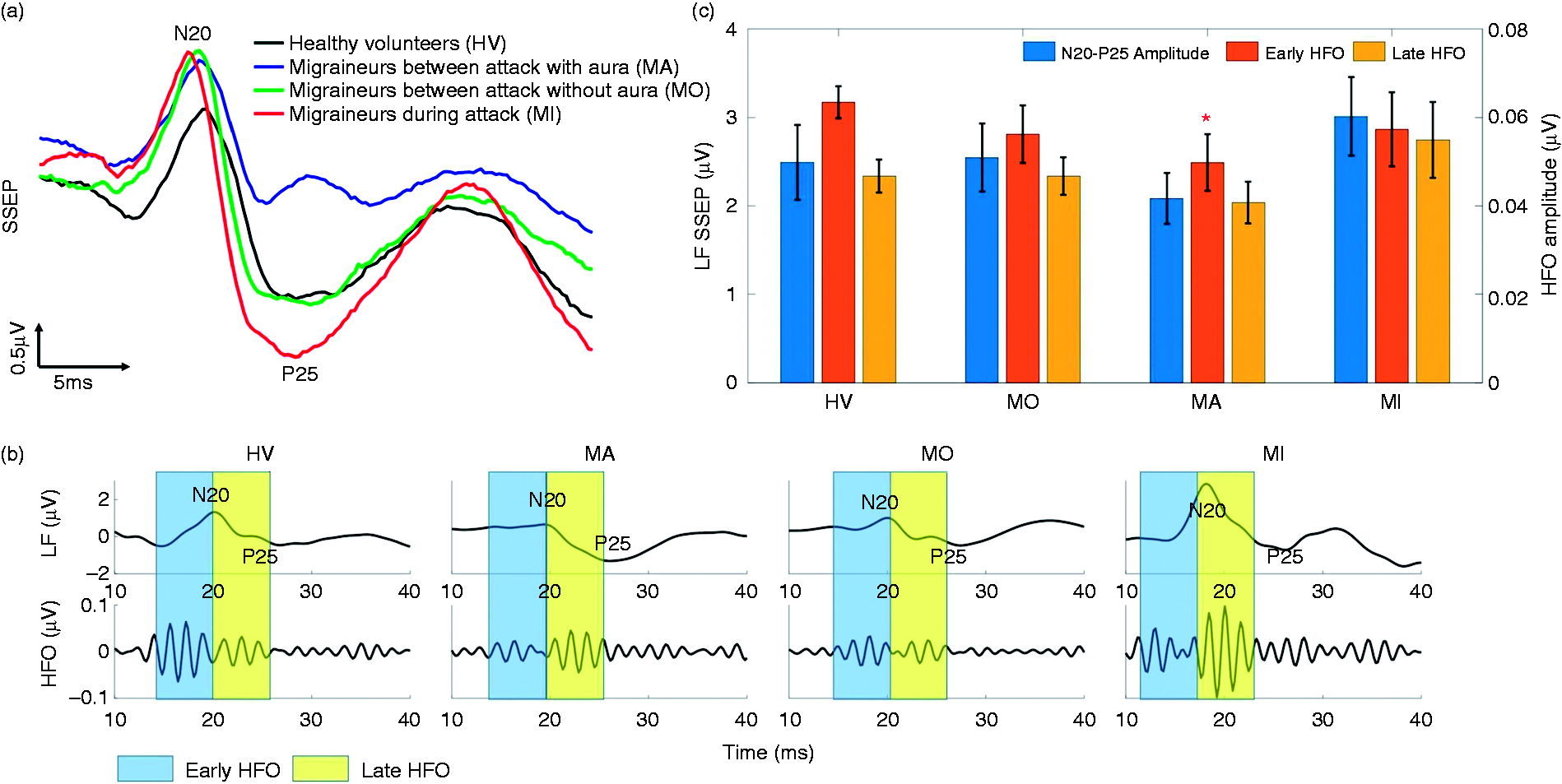

The measured SSEPs were composed of 425 to 2000 independently collected trials (Supplemental Table 2). For the purpose of feature extraction, we averaged every 40 consecutive sweeps and labelled the resulting waveform as healthy volunteer (HV), ictal (MI), or interictal (MII), depending on the subject under study. Averaging over different numbers of trials was tested to find the value that maximized the classification accuracy. This resulted in a total of 325 MI, 534 MII, and 323 HV samples that were fed to our classifiers, following feature extraction. In the feature extraction phase, each sample was independently processed to avoid data leakage between the train and test sets.

In addition to the features of HFO and LF-SSEP described above, a number of electrophysiological measures that are widely used in EEG analysis were included, such as spectral power in various frequency bands (11,26), and Hjorth parameters (22,23), as listed in Table 1. In order to reduce the effect of power fluctuations among individuals, spectral power features were normalized to each sample's total power. The Hjorth parameters, known as activity, mobility, and complexity, indicate various signal properties in the time domain. Specifically, Hjorth activity is an indicator of signal variance, while mobility represents the mean frequency. Moreover, the frequency changes over a given time period can be represented by complexity. In Supplemental Table 3, we show the mean values and standard deviation (STD) of features listed in Table 1.

Table 1.

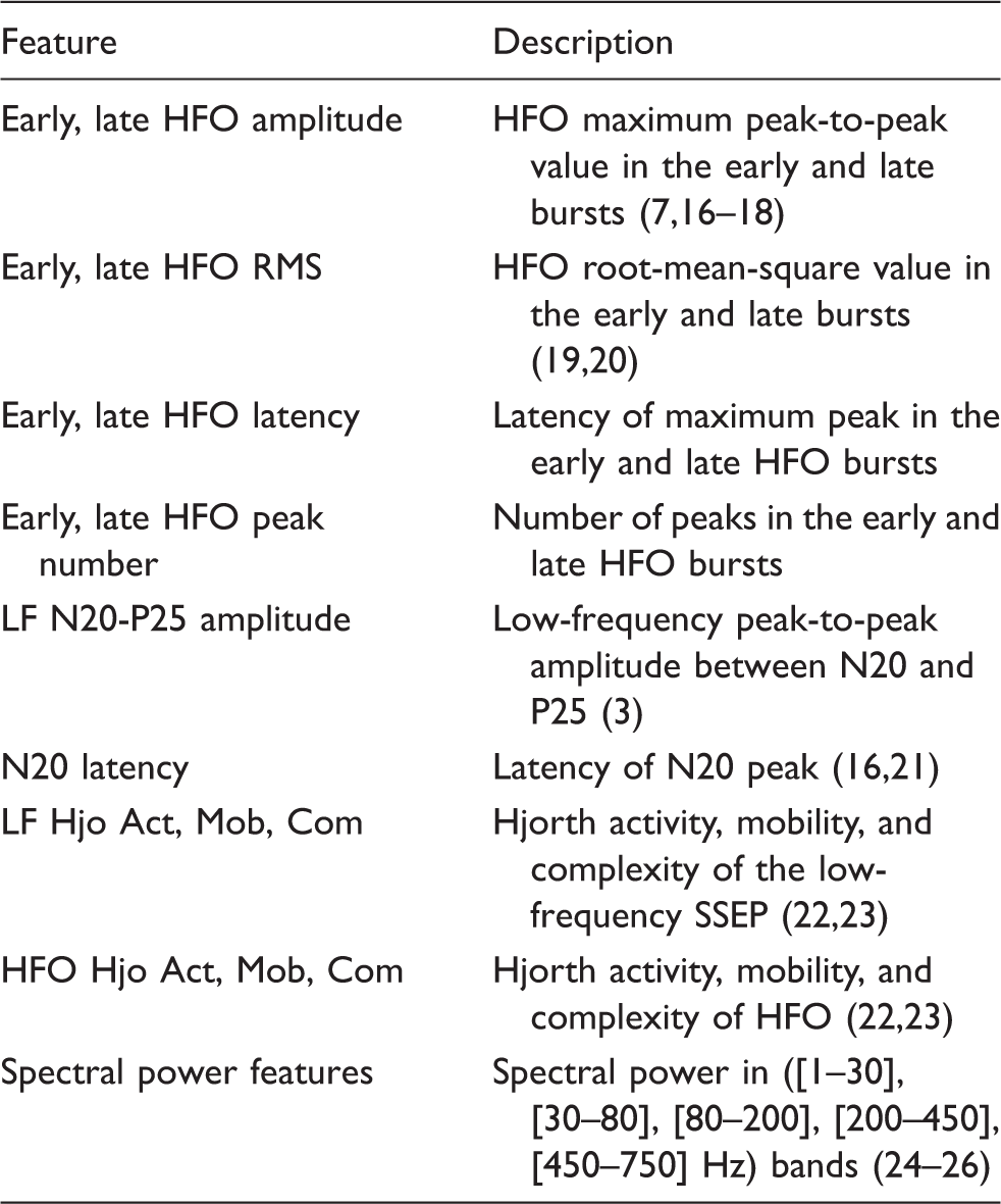
Extracted features from SSEP recordings.

Feature	Description
Early, late HFO amplitude	HFO maximum peak-to-peak value in the early and late bursts (7,16–18)
Early, late HFO RMS	HFO root-mean-square value in the early and late bursts (19,20)
Early, late HFO latency	Latency of maximum peak in the early and late HFO bursts
Early, late HFO peak number	Number of peaks in the early and late HFO bursts
LF N20-P25 amplitude	Low-frequency peak-to-peak amplitude between N20 and P25 (3)
N20 latency	Latency of N20 peak (16,21)
LF Hjo Act, Mob, Com	Hjorth activity, mobility, and complexity of the low-frequency SSEP (22,23)
HFO Hjo Act, Mob, Com	Hjorth activity, mobility, and complexity of HFO (22,23)
Spectral power features	Spectral power in ([1–30], [30–80], [80–200], [200–450], [450–750] Hz) bands (24–26)

It should be noted that compared with low-frequency SSEP, the amplitude of HFO is relatively small, making measurement noise a significant factor in HFO extraction and analysis. This is a challenge for classification tasks that employ HFOs as key characteristic features. In this study, we reduced the effect of random noise by averaging over a higher number of SSEP sweeps. However, averaging over many sweeps can reduce the number of training samples and make it impossible to reliably evaluate the classification performance. Therefore, considering the trade-off between noise and number of samples, a 40-sweep averaging was found to be optimal, which resulted in an accuracy of 36% for HFO features and a total of 1182 training samples.

Classification

In order to classify the SSEP recordings, we explored both handcrafted feature methods, where the domain knowledge is used to extract application-specific features (i.e. migraine biomarkers), and deep learning models such as convolutional neural network (CNN) that do not require prior knowledge and domain expertise. The classification performance was measured by a 10-fold cross-validation method for the prediction metrics of accuracy, F1 score, sensitivity and specificity, and was compared to prior works. For the handcrafted feature approach, the most critical features in the classification process were determined using a forward feature selection method, and compared with previous clinical findings.

Handcrafted feature methods

In machine learning based on feature engineering, extracting informative, independent, and domain-specific characteristics from data is critical. In this work, we selected a number of discriminating features for migraine based on previous SSEP studies, as described in the previous section. These features (listed in Table 1) form a numerical representation of the disease under study, called a feature space. Then, machine learning models were built on these features to classify the data. The effectiveness of features in migraine detection is represented by the performance of the classification algorithms that utilize them.

Our target classification problem was to distinguish between three groups of subjects using SSEP features: Migraine interictal (MII), migraine ictal (MI), and healthy (HV). We tested several state-of-the-art classifiers to achieve an optimal accuracy. These classifiers were optimized and parameter tuned in scikit-learn (scikit-learn.org) and include: Random forest (RF), extreme gradient-boosting trees (XGB), support vector machines (SVMs) with various kernels, K-nearest neighbors (KNN), mutilayer perceptron (MLP), linear discriminant analysis (LDA), and logistic regression (LR). We trained these supervised learning models on a set of labelled SSEP features and the performance of trained models was then evaluated on a test feature set with unknown labels. We compared the outputs of classifiers with the actual labels to assess the prediction accuracy. The performance of different classifiers was compared to find the optimal model. We further evaluated the three-class performance (i.e. MI-MII-HV) and compared it with the binary classification among every two groups of subjects (i.e. MI-HV, MII-HV, and MI-MII). As expected, the case of binary classification results in a higher accuracy. For the actual implementation of a migraine attack detection device, the transition from healthy to interictal and from interictal to ictal are particularly important. This could potentially be monitored in real time, by training the classifier on the previously recorded SSEP data from a patient.

Convolutional neural network

A challenge in neural data classification is to identify relevant features (i.e. biomarkers) that are significantly different among various states of a disease, or a cognitive or motor task. A patient-specific selection of features may be necessary to accommodate the variability of neural data among subjects. For example, in epileptic seizure detection, patient-specific features are widely used (28). Alternatively, the convolutional neural network is a typical deep learning model that does not rely on handcrafted features. For neural signals, the one-dimensional CNN (1D CNN) has been tested in brain-computer interface (BCI) and seizure detection applications (29 –31). Unlike handcrafted feature models, a CNN can be used to automatically learn the critical features from raw data and subsequently classify it. The independence from prior disease-based knowledge and human effort for feature design is a major advantage. Therefore, these models may have the potential to succeed in cases where sufficient discriminating features are not available.

We implemented a CNN based on the AlexNet architecture in TensorFlow (32,33), which is composed of five convolution layers, five max pooling layers, and a fully connected layer (github.com/tensorflow/models). We preprocessed the data by subtracting the mean and dividing it by the variance. The inputs to the model are the standardized SSEP signals after stimulation onset, and during the time segment of 10 ms ≤ t ≤ 40 ms. In each iteration, a batch of 100 samples is fed to the network and the associated weights are updated via backpropagation. We ran thousands of iterations until the cross-validation score converged to a stable value. This score is used as an estimate of accuracy and is compared with the handcrafted feature methods for model selection.

Results

Model performance

In order to evaluate the classification performance, we measured the 10-fold cros-validation scores (averaged through repeated iterations) for all the studied models (Figure 3), in which varying levels of accuracy were obtained for different machine learning models and on different tasks. Among the handcrafted feature methods, XGB achieves the best three-class discrimination accuracy of 72.4%. It also achieves an accuracy of 88.0% for the binary classification task of HV-MI, 86.5% for HV-MII, and 75.6% for MI-MII, respectively. To better assess the model performance, we separately looked into false positives (the number of healthy samples classified as migraine) and false negatives (the number of migraine samples classified as healthy), by reporting the specificity (true negative rate) and sensitivity (true positive rate) of classifiers. These criteria imply different clinical priorities in practice; for example, in a migraine or seizure detection system, we may prefer to raise a false alarm rather than missing an imminent seizure or migraine attack (34,35). Table 2 presents a comparison of performance for various machine learning models and each classification task. XGB outperforms other classifiers not only in terms of accuracy, but also sensitivity, specificity, and F1 score.

Figure 3.

The accuracy measured by 10-fold cross validation score (mean ± STD) for different tasks and various machine learning models. The algorithms are trained and tested on the entire feature set, and the classifier settings are optimized for each task.

Table 2.

The overall performance (expressed as mean ± STD) of machine learning models for different tasks measured by accuracy, sensitivity, specificity, and F1 score. All models are trained and tested on the entire feature set. For the SVM classifier, support vectors with linear, sigmoid, and RBF kernels were tested, and SVM-RBF was chosen as it outperformed other kernels in all classification tasks.

Model	Task	Accuracy	Sensitivity	Specificity	F1 score	Model parameters
XGB	HV-MI-MII	0.724 ± 0.007	0.790 ± 0.008∗	0.916 ± 0.004∗	0.715 ± 0.005	Tree count: 105 Maximum depth: 13
	HV-MI	0.880 ± 0.005	0.893 ± 0.008	0.903 ± 0.009	0.872 ± 0.007
	HV-MII	0.865 ± 0.003	0.869 ± 0.009	0.878 ± 0.005	0.859 ± 0.006
	MI-MII	0.756 ± 0.006	0.781 ± 0.006	0.715 ± 0.014	0.731 ± 0.007
RF	HV-MI-MII	0.686 ± 0.002	0.814 ± 0.011∗	0.875 ± 0.004∗	0.667 ± 0.003	Tree count: 276 Maximum depth: 10
p = 0.0335	HV-MI	0.844 ± 0.007	0.841 ± 0.007	0.840 ± 0.010	0.841 ± 0.007
	HV-MII	0.822 ± 0.009	0.845 ± 0.012	0.806 ± 0.004	0.798 ± 0.008
	MI-MII	0.744 ± 0.002	0.739 ± 0.006	0.711 ± 0.011	0.698 ± 0.003
SVM	HV-MI-MII	0.702 ± 0.006	0.778 ± 0.009∗	0.884 ± 0.004∗	0.681 ± 0.005	RBF kernel Kernel coefficient: 1/number of feature
p = 0.1176	HV-MI	0.826 ± 0.006	0.838 ± 0.005	0.814 ± 0.007	0.825 ± 0.006
	HV-MII	0.846 ± 0.005	0.857 ± 0.015	0.858 ± 0.004	0.830 ± 0.005
	MI-MII	0.735 ± 0.003	0.742 ± 0.002	0.752 ± 0.010	0.689 ± 0.004
KNN	HV-MI-MII	0.619 ± 0.005	0.595 ± 0.009∗	0.859 ± 0.002∗	0.601 ± 0.007	Number of neighbors: 5
p = 1 × 10⁻⁵	HV-MI	0.785 ± 0.011	0.780 ± 0.012	0.782 ± 0.011	0.785 ± 0.011
	HV-MII	0.783 ± 0.012	0.767 ± 0.019	0.793 ± 0.009	0.759 ± 0.014
	MI-MII	0.697 ± 0.011	0.727 ± 0.007	0.612 ± 0.018	0.662 ± 0.011
MLP	HV-MI-MII	0.684 ± 0.006	0.734 ± 0.012∗	0.888 ± 0.004∗	0.661 ± 0.005	Hidden layer size: 200
p = 0.0003	HV-MI	0.815 ± 0.007	0.799 ± 0.003	0.796 ± 0.006	0.822 ± 0.008
	HV-MII	0.833 ± 0.006	0.826 ± 0.011	0.852 ± 0.005	0.809 ± 0.006
	MI-MII	0.738 ± 0.008	0.761 ± 0.007	0.662 ± 0.015	0.723 ± 0.012
LDA	HV-MI-MII	0.532 ± 0.005	0.528 ± 0.018∗	0.772 ± 0.004∗	0.472 ± 0.007	Least squares solution with auto shrinkage
p = 4 × 10⁻⁵	HV-MI	0.685 ± 0.008	0.692 ± 0.008	0.702 ± 0.009	0.684 ± 0.008
	HV-MII	0.668 ± 0.007	0.609 ± 0.015	0.685 ± 0.005	0.597 ± 0.009
	MI-MII	0.695 ± 0.003	0.693 ± 0.003	0.671 ± 0.009	0.630 ± 0.005
LR	HV-MI-MII	0.512 ± 0.003	0.510 ± 0.011∗	0.774 ± 0.002∗	0.461 ± 0.003
p = 4 × 10⁻⁶	HV-MI	0.697 ± 0.006	0.689 ± 0.006	0.706 ± 0.007	0.696 ± 0.006	Default settings
	HV-MII	0.660 ± 0.005	0.584 ± 0.009	0.696 ± 0.004	0.604 ± 0.007	Default settings
	MI-MII	0.681 ± 0.005	0.696 ± 0.003	0.639 ± 0.011	0.622 ± 0.006

The p-values are obtained by utilizing one-way ANOVA to study the accuracy between XGB and other models. A p < 0.05 is considered significant and indicates that XGB performs significantly better than the corresponding model in all the studied tasks.

∗

The sensitivity and specificity for the HV-MI-MII classification task are measured by the one-vs-rest (OvR) method, which compares migraineurs in either ictal or interictal states with healthy controls.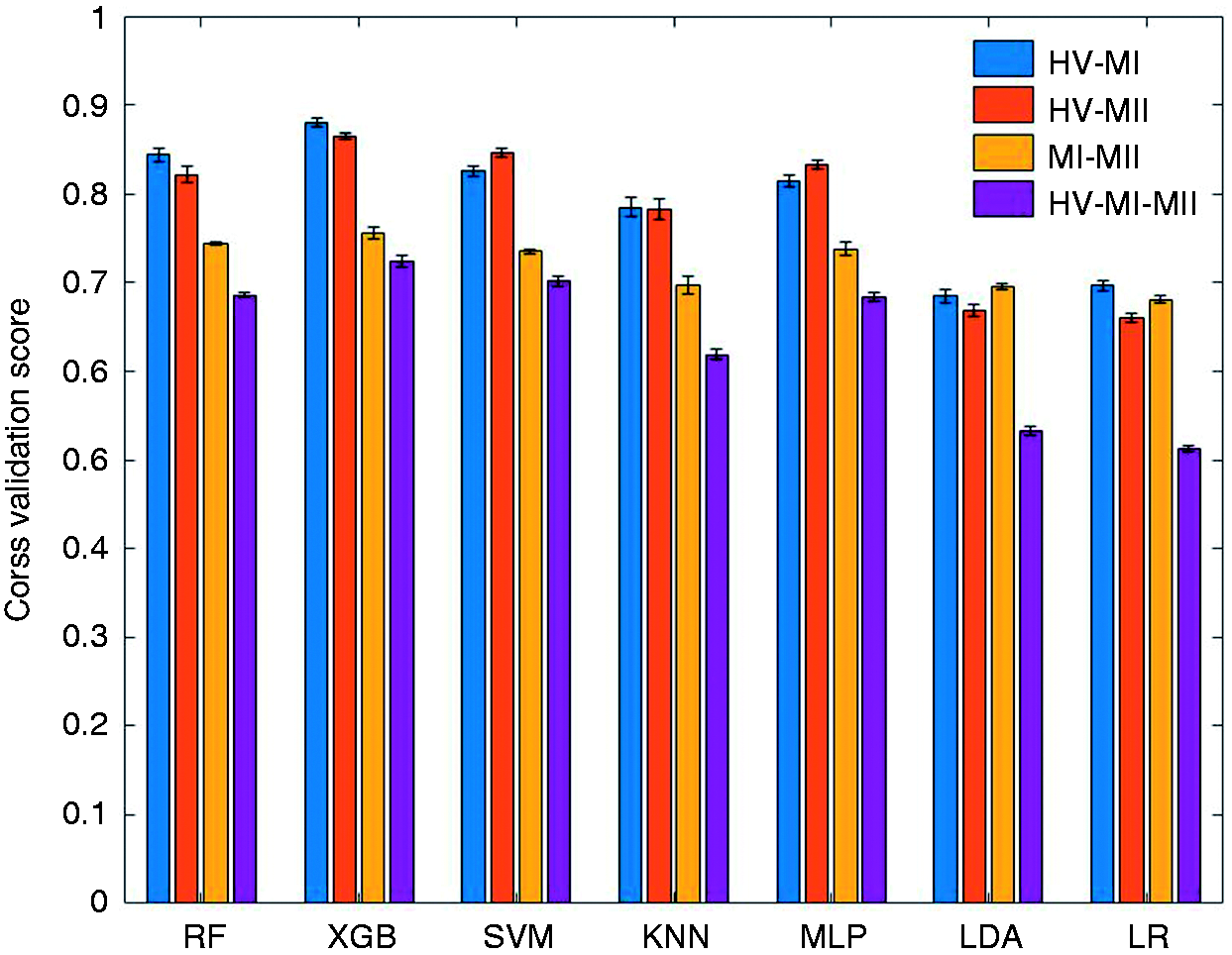

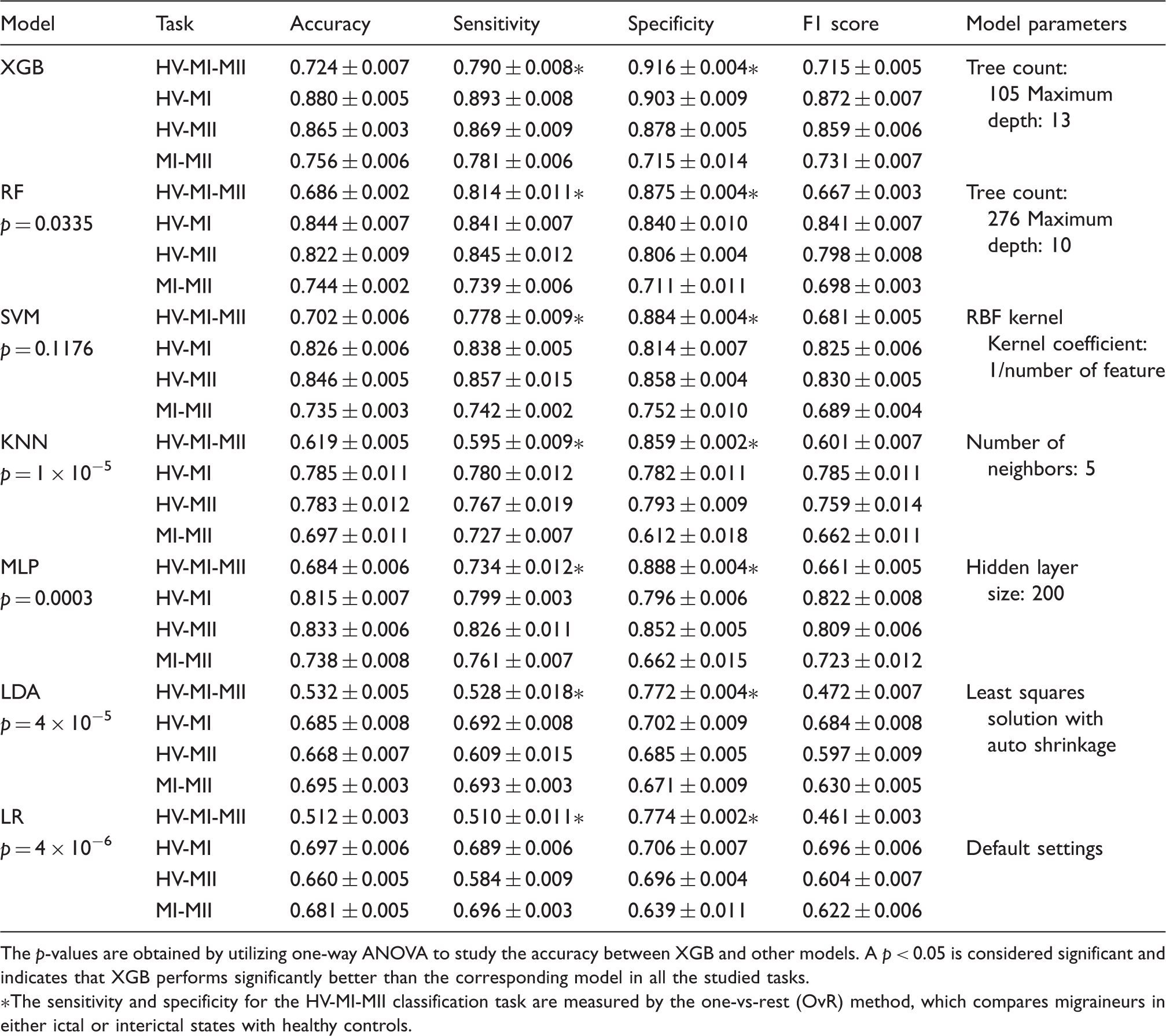
A hyperparameter tuning of classifier parameters was performed to achieve the optimal settings that lead to the highest accuracy. In order to fairly compare the performance of classifiers and select the best model, we applied one-way analysis of variance (ANOVA) between XGB and any other model. The significance level was set to p < 0.05, indicating that the two models perform significantly differently for a given classification task. From the statistical analysis presented in Table 2, we can conclude that XGB performs significantly better than RF, KNN, MLP, LDA, and LR. Compared with SVM-RBF, XGB achieves higher scores in all the metrics shown in Table 2, even though it does not reach the significance level.

We further examined the CNN to classify migraine states, but the performance was not satisfactory. This is likely due to the limited amount of training data (Figure 4). In general, while deep neural networks achieve state-of-the-art accuracy in most learning tasks that involve large datasets of unstructured data, the application of such techniques may not be beneficial in problems with limited training sets or under domain-specific test time constraints (36). With a cross-validation score of 56.3%, CNN is inferior to most handcrafted feature methods in this study, yet outperforms the linear models such as LR and LDA. The XGB classifier is the winning model in our study and is developed based on the gradient boosting technique (37,38). Ensembles of decision trees such as gradient boosting and random forests have been among the most competitive methods in machine learning recently (36), particularly in a regime of limited training data and little need for parameter tuning. In particular, the XGB implementation has been a winning solution in many machine learning competitions, such as the intracranial EEG-based seizure prediction contest on Kaggle (39), and has been included in our analysis. Gradient boosting exploits gradient-based optimization and boosting by adaptively combining many simple models (in this case, binary split decision trees) to get an improved predictive performance. To the best of our knowledge, this is the first study to explore XGB in migraine signal analysis.

Figure 4.

The train and test accuracies of the 1D-CNN model for the HV-MI-MII classification task. The cross validation score for test data converges to 56.3%, which is lower than most studied feature-based models yet better than linear models.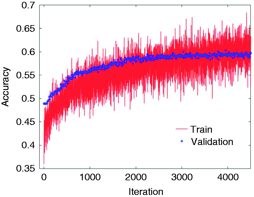

Feature selection

In machine learning, classification with fewer attributes has generally been favored, as it reduces the number of redundant (i.e. highly correlated) or marginally relevant features, in addition to reducing the computation time and hardware complexity. Feature selection and dimensionality reduction are the two widely used methods for reducing the number of attributes. Dimensionality reduction is commonly achieved by obtaining a set of principal components of features, whereas feature selection methods choose the most discriminating attributes without modifying them. Principal component analysis (PCA) is a common approach for dimensionality reduction and has been widely used in EEG preprocessing and classification (40). However, due to its unsupervised nature, the performance of PCA in supervised learning tasks may be suboptimal. In contrast, feature selection methods select a subset of relevant features for model construction, which aids in building an accurate predictive model while reducing the number of features.

Given the relatively large number of examined features in the current study, we used a forward feature selection (FFS) method to further enhance the classification accuracy and remove the redundant features. The algorithm starts by evaluating all feature subsets which consist of only one input attribute. In each iteration, the combination of prior subset and a new feature from the pool of remaining features is exhaustively explored and evaluated with a cross-validation score. The algorithm then continues to add the best feature in each iteration and update the combinational subset until the entire feature set is analyzed (41).

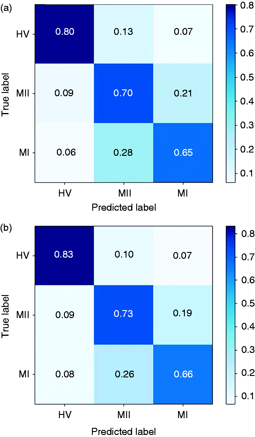
In this study, we compared the forward feature selection method with the commonly used PCA and feature importance-based selection methods. The latter approach relies on how useful each feature is in the construction of the classification model (generally decision trees). As shown in Figure 5, the FFS outperforms other methods in terms of both accuracy and convergence rate. Using FFS, we selected an optimal subset consisting of 16 features and achieved an accuracy of 73.3% for the three-class detection task. For the binary classification tasks, an accuracy of 89.7% was achieved for HV-MI (by selecting 11 features), 88.7% for HV-MII (14 features), and 80.2% for MI-MII (12 features), respectively. To better illustrate this, Figure 6 depicts the confusion matrices prior to and following forward feature selection. The confusion matrix reports the percentage of successfully classified or misclassified samples. We can see that following feature selection, the sensitivity and specificity scores have significantly improved. Overall, this method results in an average improvement of 2.4% in the classification accuracy, and a 37.0% reduction in the number of extracted features. (Supplemental Table 4 shows the selected subset of features and the gain in accuracy by adding each feature in Figure 5).

Figure 5.

The classification performance for the HV-MI-MII task versus number of features for three different feature selection methods. The mean accuracy (Mean) and standard deviation (STD) are shown as solid lines and shaded areas, respectively. The forward feature selection (FFS) approach outperforms the feature importance and PCA methods.

Figure 6.

(a) The original confusion matrix; (b) confusion matrix after feature selection. Following forward feature selection, the diagonal elements of the matrix grow larger, indicating that more samples are correctly classified. This implies that FFS effectively boosts the system performance in migraine states classification tasks, while reducing the number of redundant features.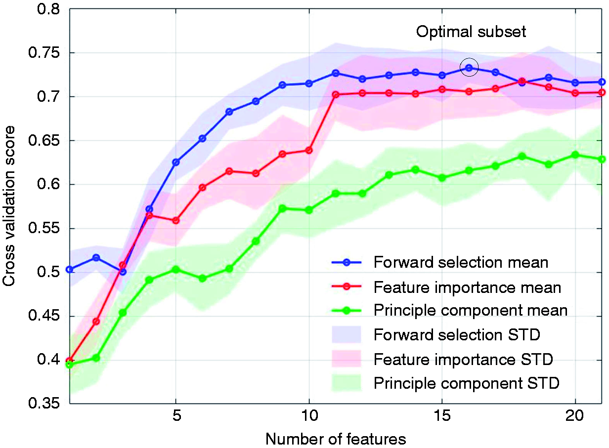

Discussion

Migraine biomarkers

To better assess the importance of various SSEP correlates of migraine in the proposed classification system, the top three discriminating features based on the FFS method are listed in Table 3. For the HV-MI detection task, the LF N20-P25 amplitude and RMS value of late HFO stand out, which is consistent with prior findings (8,20). Our study confirms that migraineurs in the ictal state have higher N20-P25 amplitude and late HFO burst (8). The HFO mobility characterizes healthy versus migraine interictal, indicating that the mean frequency of the power spectrum in the HFO band differs between the two groups. For the case of MI-MII, both early and late HFO bursts play a key role. The other important feature is the latency of the N20 peak. While the N20 latency is not widely covered in migraine literature, some studies report that it changes during migraine treatment (21). This motivates the use of N20 latency in our migraine classification system. Besides, the N20 latency is largely stable over time, even when averaged over a relatively small number of SSEP recordings. Based on our results, the N20 latency might be a potentially prominent feature for migraine classification. We further observe that the broadband gamma (80–200 Hz) as well as HFO (450–750 Hz) frequency bands are important for HV-MII and HV-MI-MII classification tasks, respectively.

Table 3.

The top performing features based on FFS method.

Classification task	Top features
HV-MI-MII	N20 latency,
	late HFO RMS,
	Spectral power in [450–750] Hz.
HV-MI	LF N20-P25 amplitude,
	N20 latency,
	Late HFO RMS.
HV-MII	N20 latency,
	Spectral power in [80–200] Hz,
	HFO Hjo Mob.
MI-MII	N20 latency,
	Late HFO latency,
	Early HFO peak numbers.

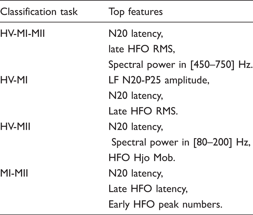
The single-feature classification accuracy for the studied features is illustrated in Figure 7, using a 10-fold cross validation score and XGB classifier. The single-feature accuracy is obtained in the first step of the feature selection routine and could be used to estimate the feature importance. However, combining the top performing features based on single-feature accuracy does not necessarily lead to the most optimal feature set. In contrast, the employed feature selection method accounts for the mutual information and correlation among features to find the optimal subset. For instance, there is a high correlation among features that pertain to similar aspects of a signal, such as HFO amplitude and RMS. Therefore, the forward selection method is preferred to the single-feature importance method to build a subset of discriminating features.

Figure 7.

The single-feature accuracies (mean ± STD) of the studied feature set. These scores represent a measure of effectiveness of individual features in the classification task. Lat: latency; Amp: amplitude; NoP: number of peaks; NSP: normalized spectral power.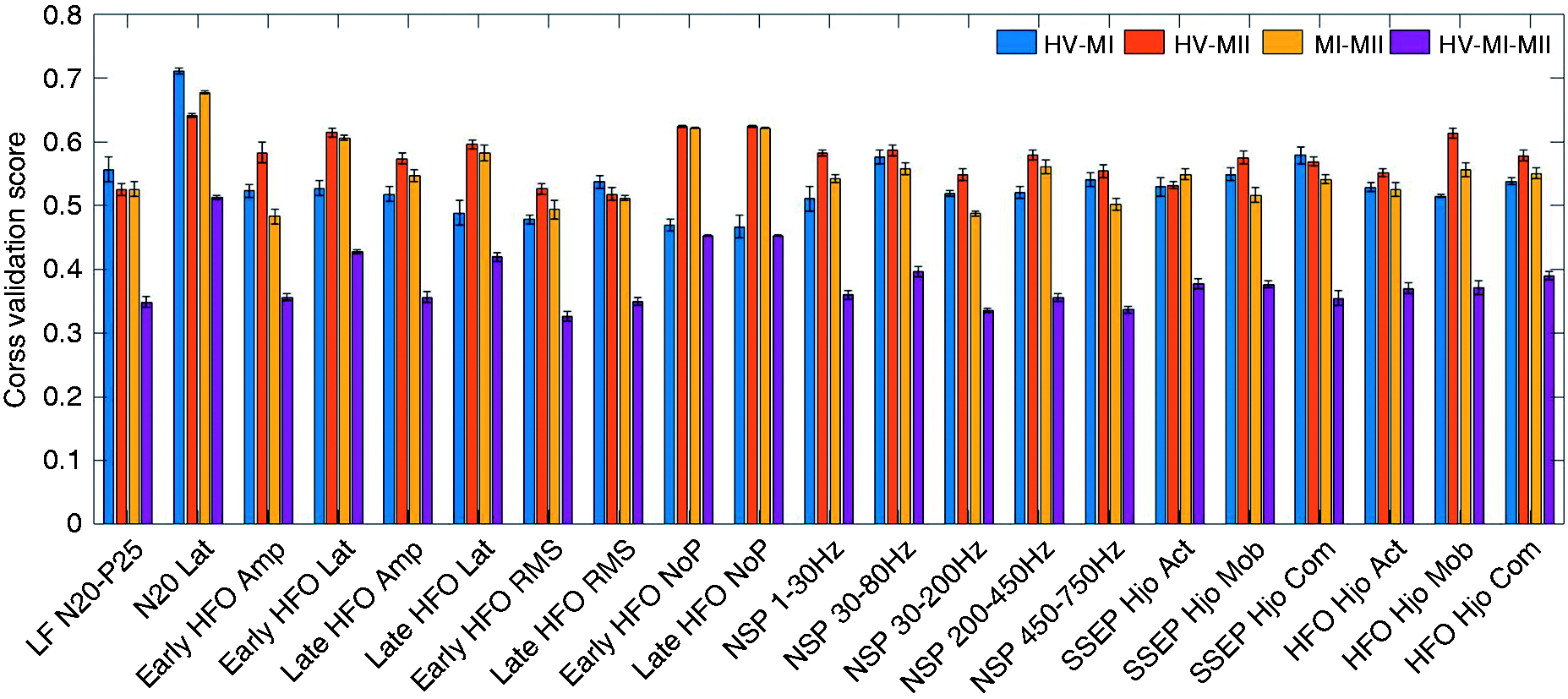

For migraineurs during attack, prior studies report that the N20-P25 amplitude of LF-SSEP is higher than healthy controls (8,42). This is confirmed by the superior performance of the N20-P25 feature in MI-HV classification. Moreover, the primary cortical activation represented by late HFOs is shown to increase in the ictal state (8). We also observe that the late HFO RMS is a powerful feature in the HV-MI classification task. On the other hand, the reduced amplitude of the early HFO burst reflects a decrease in somatosensory thalamo-cortical activity (43). It is likely that the reduction of pre-activation level in sensory cortices leads to habituation deficit in the migraine interictal state (7). This could possibly explain the high single-feature accuracy of early HFO features in the HV-MII classification task. Another finding in Table 3 is that while the interictal group exhibits reduced early HFOs, the amplitude of early HFO is not a key indicator of the migraine ictal group. This is further verified by the single-feature performance shown in Figure 7. In other words, the features of early HFO are more effective in separating the interictal group from healthy controls. This is due to the fact that the thalamo-cortical activation reflected by early HFOs starts to normalize during the ictal state. Yet, the MI group has relatively larger late HFOs compared to the HV and MII groups.

Comparison to prior works

In Table 4, we summarize the performance of the proposed method and compare it to prior works on classification of migraine phases. To the best of our knowledge, this is the first SSEP-based migraine state classification system. As shown in this table, various other signal modalities have been previously explored for detection of migraine states. The resting fMRI in ictal migraineurs and healthy controls was recently studied (15). Compared with fMRI, SSEPs are easier to collect and analyze in real time. Alternatively, resting-state EEGs and visual evoked potentials (VEPs) have been previously used for migraine detection (12,44). However, these studies rely on multiple channels of input data, which can hinder their integration into a low-cost and portable monitoring device. In this paper, the classification tasks are performed using a single-channel SSEP signal, making the proposed system more effective and convenient for patient use. We attain a relatively high accuracy of above 88% in migraine ictal or interictal versus healthy discrimination (HV-MI, HV-MII), and above 80% in classification of two migraine states (MI-MII). Therefore, the proposed algorithm promises a potential to predict migraine attacks in advance, making early intervention possible for more effective migraine treatment.

Table 4.

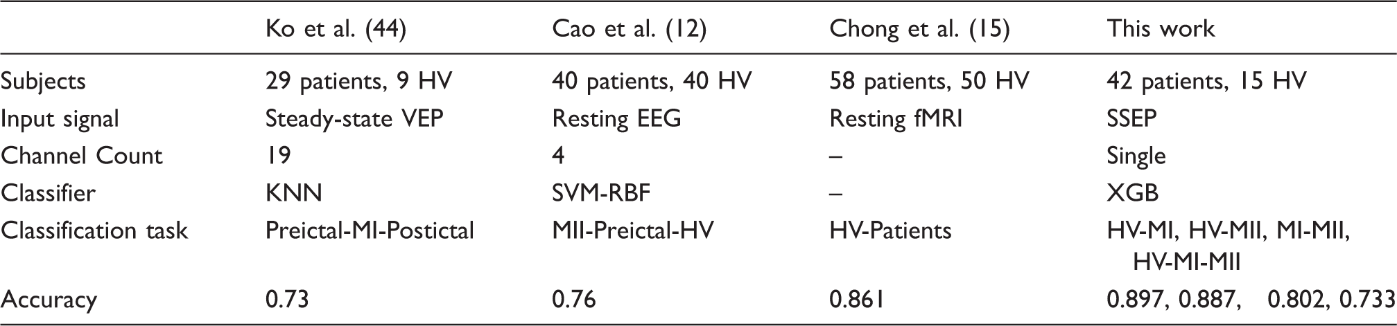
Performance summary and comparison with prior work on migraine classification.

	Ko et al. (44)	Cao et al. (12)	Chong et al. (15)	This work
Subjects	29 patients, 9 HV	40 patients, 40 HV	58 patients, 50 HV	42 patients, 15 HV
Input signal	Steady-state VEP	Resting EEG	Resting fMRI	SSEP
Channel Count	19	4	–	Single
Classifier	KNN	SVM-RBF	–	XGB
Classification task	Preictal-MI-Postictal	MII-Preictal-HV	HV-Patients	HV-MI, HV-MII, MI-MII, HV-MI-MII
Accuracy	0.73	0.76	0.861	0.897, 0.887, 0.802, 0.733

Limitations

Despite promising results, our current study has several limitations. While some of the analyzed biomarkers are supported by prior studies (7,8,17 –19), the reliability of classifiers and statistical significance of the achieved results need to be verified on more patients and long-term recordings. Limited by the availability of data, we were not able to separately study the migraine preictal and postictal states, which could be important in migraine attack prediction. Therefore, the proposed classification system should be tested on more patients and various migraine phases in future.

In addition, the individual differences among subjects might affect our analysis and similar studies that are performed across subjects. For example, N20 latency was reported to correlate with height and brain size (45), which are not included in our study. A single-subject analysis in different phases of migraine is preferred to design a personalized migraine classification system. Here, we tried to minimize the impact of individual differences by using normalized spectral power features and standardized SSEPs. Given that the top performing features are well consistent with published works, we may conclude that individual differences do not play a major role in our analysis. Most importantly, while this study and previous works in Table 4 allow us to assess the separability of various migraine states among individuals, the practical design of a headache monitoring system requires the use of continuous data from a single subject. In our future work, we will test a patient-specific classification approach on the long-term and multistate data from individual patients in order to predict the transition from one state of migraine to another. This would be similar to the patient-specific seizure monitoring systems for medication-resistant epilepsy (46).

Conclusion

In this study, we proposed a new SSEP-based system for migraine classification. Machine learning approaches were combined with an efficient feature selection method, not only to achieve a decent classification performance, but also to provide a systematic solution for feature importance assessment. Overall, we were able to achieve over 88% accuracy in migraine ictal or interictal versus healthy detection. We tested a recently developed and highly competitive class of boosting algorithms to classify migraineurs in ictal and interictal states. This XGB framework outperforms most widely used models in our analysis. Furthermore, the proper selection of features can reduce the computational complexity by 37% on average, while improving the classification accuracy by 2.4%. From a clinical perspective, the study of discriminating SSEP biomarkers and their correlation with migraine phases may further reveal the potential mechanisms underlying migraine attacks. The proposed system could be used as a noninvasive headache monitoring system for early diagnosis and treatment of underlying migraine headaches.

Supplemental Material

Supplemental material for Migraine classification using somatosensory evoked potentials

Supplemental Material for Migraine classification using somatosensory evoked potentials by Bingzhao Zhu, Gianluca Coppola and Mahsa Shoaran in Cephalalgia

Footnotes

Article highlights

The proposed SSEP-based classification system offers the potential for noninvasive detection of migraine phases.

Various biomarkers of migraine ictal and interictal states are studied in a machine learning framework, which may further reveal the potential mechanisms underlying migraine attacks.

Acknowledgements

We thank Dr. Lin Yao for his valuable comments on this work.

Declaration of conflicting interests

The authors declare no potential conflicts of interest with respect to the research, authorship, and/or publication of this article.

Funding

The authors disclosed receipt of the following financial support for the research, authorship, and/or publication of this article: This work was supported by the Swiss NSF Fellowship under Grant P300P2_171220. The contribution of the G.B. Bietti Foundation in this paper was supported by the Italian Ministry of Health and Fondazione Roma.

References

Coppola

Di Lorenzo

Schoenen

et al.

Habituation and sensitization in primary headaches. J Headache Pain 2013; 14: 65.

Restuccia

Vollono

del Piero

et al.

Different levels of cortical excitability reflect clinical fluctuations in migraine. Cephalalgia 2013; 33: 1035–1047. .

Coppola

De Pasqua

Pierelli

et al.

Effects of repetitive transcranial magnetic stimulation on somatosensory evoked potentials and high frequency oscillations in migraine. Cephalalgia 2012; 32: 700–709.

Foley

Cady

Martin

et al.

Treating early versus treating mild: Timing of migraine prescription medications among patients with diagnosed migraine. Headache 2005; 45: 538–545.

Shoaran M, Shahshahani M, Farivar M, et al. A 16-channel 1.1 mm² implantable seizure control soc with sub-μw/channel consumption and closed-loop stimulation in 0.18 μm cmos. Presented at: IEEE symposium on VLSI circuits, Honolulu, HI, USA, 15–17 June 2016, pp.1–2.

Chen

Chiueh

Chen

et al.

A fully integrated 8- channel closed-loop neural-prosthetic cmos soc for real-time epileptic seizure control. IEEE J Solid-State Circ 2014; 49: 232–247.

Coppola

Vandenheede

Di Clemente

et al.

Somatosensory evoked high-frequency oscillations reflecting thalamo-cortical activity are decreased in migraine patients between attacks. Brain 2005; 128: 98–103.

Coppola

Iacovelli

Bracaglia

et al.

Electrophysiological correlates of episodic migraine chronification: Evidence for thalamic involvement. J Headache Pain 2013; 14: 76.

De Tommaso

Ambrosini

Brighina

et al.

Altered processing of sensory stimuli in patients with migraine. Nat Rev Neurol 2014; 10: 144–2 .

10.

Curio

. Linking 600-hz spikelike eeg/meg wavelets (ς-bursts) to cellular substrates: Concepts and caveats. J Clin Neurophys 2000; 17: 377–396.

11.

Park

Luo

Parhi

et al.

Seizure prediction with spectral power of EEG using cost-sensitive support vector machines. Epilepsia 2011; 52: 1761–1770.

12.

Cao

Lai

Lin

et al.

Exploring resting-state EEG complexity before migraine attacks. Cephalalgia 2018; 38: 1296–1306.

13.

Cao ZH, Ko LW, Lai KL, et al. Classification of migraine stages based on resting-state EEG power. Presented at: IEEE International Joint Conference on Neural Networks (IJCNN), Killarney, Ireland, 12–17 July 2015, pp.1–5.

14.

Sayyari E, Farzi M, Estakhrooeieh RR, et al. Migraine analysis through EEG signals with classification approach. Presented at: 11th IEEE International Conference on Information Science, Signal Processing and their Applications (ISSPA), Montreal, QC, Canada, 2–5 July 2012, pp.859–863.

15.

Chong

Gaw

et al.

Migraine classification using magnetic resonance imaging resting-state functional connectivity data. Cephalalgia 2017; 37: 828–844.

16.

Schoenen

. Neurophysiological features of the migrainous brain. Neurol Sci 2006; 27: s77–s81.

17.

Coppola

Bracaglia

Di Lenola

et al.

Lateral inhibition in the somatosensory cortex during and between migraine without aura attacks: Correlations with thalamocortical activity and clinical features. Cephalalgia 2016; 36: 568–578.

18.

Porcaro

Di Lorenzo

Seri

et al.

Impaired brainstem and thalamic high-frequency oscillatory EEG activity in migraine between attacks. Cephalalgia 2017; 37: 915–926.

19.

Sakuma

Takeshima

Ishizaki

et al.

Somatosensory evoked high-frequency oscillations in migraine patients. Clin Neurophys 2004; 115: 1857–1862.

20.

Restuccia

Vollono

Del Piero

et al.

Somatosensory high frequency oscillations reflect clinical fluctuations in migraine. Clin Neurophys 2012; 123: 2050–2056.

21.

Hamed

. A migraine variant with abdominal colic and Alice in Wonderland syndrome: A case report and review. BMC Neurol 2010; 10: 2.

22.

Hjorth

. EEG analysis based on time domain properties. Electroenceph Clin Neurophys 1970; 29: 306–310.

23.

Vourkas M, Micheloyannis S and Papadourakis G. Use of ann and hjorth parameters in mental-task discrimination. Presented at: IET First International Conference Advances in Medical Signal and Information Processing (IEE Conf. Publ. No. 476), Bristol, UK, 4–6 September 2000, pp.327–332.

24.

Sarnthein

Stern

Aufenberg

et al.

Increased EEG power and slowed dominant frequency in patients with neurogenic pain. Brain 2005; 129: 55–64.

25.

Walker

. QEEG-guided neurofeedback for recurrent migraine headaches. Clin EEG Neurosci 2011; 42: 59–61.

26.

Staba

Stead

Worrell

. Electrophysiological biomarkers of epilepsy. Neurotherapeutics 2014; 11: 334–346.

27.

Inoue

Hashimoto

Shirai

et al.

Disinhibition of the somatosensory cortex in cervical dystonia decreased amplitudes of high-frequency oscillations. Clin Neurophys 2004; 115: 1624–1630.

28.

Zhang

Parhi

. Low-complexity seizure prediction from iEEG/sEEG using spectral power and ratios of spectral power. IEEE Trans Biomed Circ Sys 2016; 10: 693–706.

29.

Li D, Zhang J, Zhang Q, et al. Classification of ECG signals based on 1D convolution neural network. Presented at: IEEE 19th International Conference on e-Health Networking, Applications and Services (Healthcom), Dalian, China, 12–15 October 2017, pp.1–6.

30.

Cecotti H and Graeser A. Convolutional neural network with embedded Fourier transform for EEG classification. Presented at: IEEE 19th International Conference on Pattern Recognition (ICPR), Tampa, FL, USA, 8–11 December 2008, pp.1–4.

31.

Maddula R, Stivers J, Mousavi M, et al. Deep recurrent convolutional neural networks for classifying P300 BCI signals. In: Proceedings of the 7th Graz Brain-Computer Interface Conference, Graz, Austria, 18–22 September 2017, pp.18–22.

32.

Krizhevsky A, Sutskever I and Hinton GE. Imagenet classification with deep convolutional neural networks. Presented at: Advances in Neural Information Processing Systems (NIPS), Stateline, NV, USA, 3–8 December 2012, pp.1097–1105.

33.

Tian Y, Luo P, Wang X, et al. Deep learning strong parts for pedestrian detection. In: Proceedings of the IEEE International Conference on Computer Vision (ICCV), Santiago, Chile, 13–16 December 2015, pp.1904–1912.

34.

Schölkopf B, Burges CJ, Smola AJ (eds). Advances in kernel methods: support vector learning. 1st ed. Cambridge, MA: MIT press, 1999, pp. 23–127.

35.

Mormann

Andrzejak

Elger

et al.

Seizure prediction: The long and winding road. Brain 2006; 130: 314–333.

36.

Shoaran

Haghi

Taghavi

et al.

Energy-efficient classification for resource-constrained biomedical applications. IEEE J Emerg Select Topics Circuits Syst (JETCAS) 2018. 8: 693–707. .

37.

Friedman JH. Greedy function approximation: A gradient boosting machine. Ann Stat 2001; 29: 1189–1232.

38.

Chen T. Introduction to boosted trees. University of Washington Computer Science 2014; 22: 115.

39.

Google, Inc. Kaggle, www.kaggle.com (2002, accessed 26 November 2018).

40.

Subasi

Gursoy

. EEG signal classification using PCA, ICA, LDA and support vector machines. Exp Sys App 2010; 37: 8659–8666.

41.

Jain

Zongker

. Feature selection: Evaluation, application, and small sample performance. IEEE Trans Pattern Analys Machine Intel 1997; 19: 153–158.

42.

Coppola

Curra

Di Lorenzo

et al.

Abnormal cortical responses to somatosensory stimulation in medication-overuse headache. BMC Neurol 2010; 10: 126.

43.

Schoenen

. Is chronic migraine a never-ending migraine attack? Pain 2011; 152: 239–240.

44.

Ko LW, Lai KL, Huang PH, et al. Steady-state visual evoked potential based classification system for detecting migraine seizures. Presented at: 6th International IEEE/EMBS Conference on Neural Engineering (NER), San Diego, CA, USA, 6–8 November 2013, pp.1299–1302.

45.

Allison

Wood

Goff

. Brain stem auditory, pattern-reversal visual, and short-latency somatosensory evoked potentials: Latencies in relation to age, sex, and brain and body size. Electroenceph Clin Neurophys 1983; 55: 619–636.

46.

Shoeb AH and Guttag JV. Application of machine learning to epileptic seizure detection. In: Proceedings of the 27th International Conference on Machine Learning (ICML-10), Haifa, Israel, 21–24 June 2010, pp.975–982.

Supplementary Material

Please find the following supplemental material available below.

For Open Access articles published under a Creative Commons License, all supplemental material carries the same license as the article it is associated with.

For non-Open Access articles published, all supplemental material carries a non-exclusive license, and permission requests for re-use of supplemental material or any part of supplemental material shall be sent directly to the copyright owner as specified in the copyright notice associated with the article.

0.00 MB

0.15 MB