Migraine classification using magnetic resonance imaging resting-state functional connectivity data

Abstract

Background

This study used machine-learning techniques to develop discriminative brain-connectivity biomarkers from resting-state functional magnetic resonance neuroimaging (rs-fMRI) data that distinguish between individual migraine patients and healthy controls.

Methods

This study included 58 migraine patients (mean age = 36.3 years; SD = 11.5) and 50 healthy controls (mean age = 35.9 years; SD = 11.0). The functional connections of 33 seeded pain-related regions were used as input for a brain classification algorithm that tested the accuracy of determining whether an individual brain MRI belongs to someone with migraine or to a healthy control.

Results

The best classification accuracy using a 10-fold cross-validation method was 86.1%. Resting functional connectivity of the right middle temporal, posterior insula, middle cingulate, left ventromedial prefrontal and bilateral amygdala regions best discriminated the migraine brain from that of a healthy control. Migraineurs with longer disease durations were classified more accurately (>14 years; 96.7% accuracy) compared to migraineurs with shorter disease durations (≤14 years; 82.1% accuracy).

Conclusions

Classification of migraine using rs-fMRI provides insights into pain circuits that are altered in migraine and could potentially contribute to the development of a new, noninvasive migraine biomarker. Migraineurs with longer disease burden were classified more accurately than migraineurs with shorter disease burden, potentially indicating that disease duration leads to reorganization of brain circuitry.

Introduction

Migraine pain is a complex and subjective experience that includes sensory-discriminative, affective, and cognitive aspects. Neuroimaging studies have shown functional alterations in the migraine brain in widespread brain regions involved in pain processing (1–10). These functional brain alterations are evident in the ictal as well as the interictal phase, thus suggesting that migraine might have a characteristic functional “brain-signature.” Resting-state functional magnetic resonance imaging (rs-fMRI) has been useful for delineating the neural underpinnings of the pain experience in migraine patients. An increasing body of literature has shown people with migraine to have alterations in the functional connectivity (fc) of regions important for mediating sensory, affective, and cognitive components of pain (11–13).

Machine-learning algorithms trained to automatically classify patient populations from healthy controls based on rs-fMRI measures have shown good utility for discriminating patients with chronic pain such as chronic back pain, fibromyalgia, rheumatoid arthritis or functional dyspepsia (14–16) from healthy controls, yet rs-fMRI measures have not yet been used as input metrics for accurately discriminating migraine patients from healthy controls. The ability to classify individual migraine patients from healthy controls based on rs-fMRI patterns would provide objective insight into the neural mechanism of migraine and would potentially provide an objective brain biomarker for migraine.

The objective of this study was to develop a brain classification model to distinguish individual migraine patients from healthy controls based on resting-state functional connectivity (rs-fc) patterns derived from magnetic resonance (MR) imaging data.

Methods

A total of 108 individuals (58 migraineurs and 50 healthy controls) were recruited for study participation from two medical institutions: Mayo Clinic Arizona and Washington University School of Medicine in St. Louis. This study was approved by the local institutional review boards and all participants gave informed consent prior to their participation in the study. Exclusion criteria included the presence of neurological disease other than migraine—for the migraine population, psychiatric disease or the presence of head trauma. All migraine patients were diagnosed with episodic or chronic migraine according to the diagnostic criteria set forth by the International Classification of Headache Disorders (ICHD-II) (17). Healthy controls consisted of community-dwelling individuals who never had migraines. Healthy controls were included if they never developed headaches or if they had occasional tension-type headaches with a frequency of less than three tension-type headaches per month. Additionally, none of the patients took opiates for pain relief or took migraine-preventive medications and all migraine patients stated they had migraines for a minimum of three years. All imaging and diagnostic assessments were conducted during a single two-and-a-half-hour visit. Individuals were excluded from the final analysis if they developed a headache in the scanner or if they stated having a migraine less than 48 hours prior to testing. All participants completed the Beck Depression Inventory (BDI-II) (18), and the State/Trait Anxiety Inventory (STAI, Form Y-1 and Form Y-2) (19) to assess levels of depression and anxiety, respectively.

Demographic data of migraine patients and healthy control cohorts were compared using t-tests (two-tailed) or Fisher’s exact test, as appropriate.

Imaging parameters

All high-resolution T1- and T2-weighted imaging was conducted on 3-Tesla Siemens (Erlangen, Germany) scanners using Food and Drug Administration (FDA)-approved sequences with the following parameters:

Washington University (3T Siemens MAGNETOM Trio): T1-weighted imaging; repetition time (TR) = 2400 ms; echo time (TE) = 3.16 ms; flip angle = 8 degrees. T2-weighted imaging; TE = 88 ms, TR = 6280 ms, flip angle = 120 degrees, 1 × 1 × 4 mm³ voxels

Blood-oxygen-level-dependent (BOLD) resting-state; TE=25 ms, TR=2500 ms, 4.0x4.0x4.0 mm³ voxels Mayo Clinic (3T Siemens MAGNETOM Skyra): T1-weighted imaging; TR = 2400 ms; TE = 3.06 ms; (TI) = flip angle = 8 degrees. T2-weighted imaging; TE = 84 ms, TR = 6800 ms, flip angle = 150 degrees, 1 × 1 × 4 mm³ voxels; BOLD resting-state; TE=27 ms, TR=2500 ms, 4.0 × 4.0 × 4.0 mm³ voxels.

All imaging was reviewed and individuals with structural abnormalities seen on T1-weighted imaging were excluded from the final data analysis. Migraine patients and healthy controls were continuously enrolled into the study at both sites. Migraine patients and healthy controls were scanned during a period of 18 months at Mayo Clinic, and during a period of 24 months at Washington University. No scanner updates were performed during these time periods at either institution.

Data collection and resting-state preprocessing

Ten minutes of rs data were collected for each individual. Prior to the beginning of the scanning sequence, participants were reminded to relax, to remain motionless, and to stay awake but to keep their eyes closed. It is of note that there is still little consensus as to the optimal rs condition (“eyes closed” versus “eyes open” versus “eyes fixated on a cross-hair”) although recent results by Patriat at al. (20) suggest no significant differences in connectivity strength among these conditions for most rs networks, albeit slightly higher connectivity in the auditory network in the eyes-closed condition. We chose the “eyes-closed” condition for the current study because the instructions are easy to give and easy to understand for the subjects. Participants were also given the following instructions prior to the rs run: “Please stay awake, but close your eyes and clear your mind.”

To avoid post-processing irregularities, all individuals were post-processed on a single Macintosh computer running OS X Lion 10.7.5 software using SPM 8 (Wellcome Department of Cognitive Neurology, Institute of Neurology, London, UK) and DPARSF (21) that was interfaced with MATLAB version 11.0 (MathWorks, Natick, MA, USA).

Standard SPM methodology was used to preprocess rs data, which included the following steps: (a) slice-time correction; (b) motion correction (22), and re-alignment to the first volume; (c) skull and non-brain tissue removal; (d) spatial smoothing (6 mm, full width at half maximum (FWHM)); (e) functional scans were first realigned to each person’s own structural (T1-weighted) volumes and then warped to the standardized Montreal Neurological Institute (MNI)305 template to allow for signal averaging across all subjects (23). Data were band-pass filtered within SPM using a discrete cosine transform between 0.01 to 0.1 Hz to retain the low-frequency components of the signal (24). Variance relating to signals of no interest was removed from the rs data through linear regression. These included: white matter signal, cerebrospinal fluid signal and global mean signal. Head motion was regressed out using a framewise displacement model on the surface of a 50 mm radius sphere (25). Movement calculation was conducted within DPARSF and indicated no differences in scanner motion between healthy controls and migraine patients. As there might be concern that scanner movement could potentially be correlated with the division into groups, we conducted a post-hoc analysis that indicated that only three control individuals and four migraine patients showed more than 0.5 mm movement. This indicates that scanner movement was not specifically related to one group and as such did not affect correlation results.

Finally, we applied a seed-based (region of interest (ROI)) correlation analysis and computed Fisher r-z transformation maps by extracting the time courses over each seed region (total of 33 seed regions) and computing the correlation of each seed region with each voxel throughout the brain. As rs data are susceptible to movement artifacts (26), all scans were checked for motion and those that exceeded 2.0 mm in movement were excluded from the final analysis.

The selection of the 33 areas that were selected for the current study was based on findings in the pain and migraine literature. The selected regions are those that are consistently shown to participate in pain processing. Many of these pain-processing regions have been previously shown by other investigators to have atypical structure or function in migraineurs compared to healthy controls (27–29). The precise x,y,z coordinates for these regions were then determined using the MNI Atlas, and an 8 mm sphere was drawn around the x,y,z coordinates of each of these regions to explore the functional connectivity of these ROIs with every voxel in the brain.

Sixteen brain areas of interest were selected over each hemisphere as well as one midline area (periaqueductal gray) for a total of 33 brain areas. See Table 1.

Table 1.

Thirty-three regions of interest (ROIs).

	MNI coordinates
Regions	X	Y	Z
Anterior insula	+/−38	19	−3
Anterior cingulate	+/−6	28	24
Middle cingulate	+/−10	−7	46
Posterior insula	+/−40	−14	1
Posterior cingulate	+/−8	−48	39
Thalamus	+/−8	−21	7
Primary somatosensory	+/−46	−24	47
DLPFC	+/−40	39	24
Inferior lateral parietal	+/−57	−48	30
VMPFC	+/−6	36	−14
Secondary somatosensory	+/−52	−28	21
Somatomotor	+/−6	1	68
Temporal pole	+/−41	10	−32
Amygdala	+/−22	−1	−22
Middle temporal	+/−60	−26	−5
Periaqueductal gray	a −1	−26	−11
Caudate	+/−14	13	11

DLPFC: dorso-lateral prefrontal-cortex; VMPFC: ventromedial-prefrontal-cortex. All X, Y, Z-coordinates are labeled in Montreal Neurological Institute (MNI) space. Functional connectivity was explored for all ROIs using an 8-mm sphere.

(+/−) indicates right or left hemispheric regions.

a

Indicates a midline structure.

Brain classification pipeline

An overview of our analysis pipeline is shown in a flow diagram (Figure 1.) We used an ROI approach to estimate whole-brain connectivity of 33 a priori selected ROIs in migraine patients and healthy controls. These ROIs were selected based on published findings of commonly described changes in functional connectivity and brain activation patterns in migraine patients. Rs connectivity maps were calculated by extracting the time courses of each of the 33 seeded regions with every voxel in the brain (Fisher r-z transformation maps). Important principal components as defined below were then extracted from the Fisher r-z transformation maps and applied to a machine-learning classification algorithm to test the accuracy of distinguishing between migraine patients and healthy controls.

Figure 1.

Flow diagram for the functional magnetic resonance neuroimaging (fMRI) data analysis (Step 1) and the machine-learning classification (Step 2).

Statistical analysis

Our rs analysis included the interrogation of the functional connectivity of each ROI with every voxel in the brain. Initially the voxels were mapped into a commonly used brain atlas (obtained from talairach.org) and 4484 points that were labeled as “No Gray Matter” were eliminated from the total set of 70,831 voxels. Per ROI, this analysis generates 66,347 data points, which are statistically difficult to interpret. Therefore, a principal component analysis (PCA) was used to reduce the dimensions of the data. After creating new features that are a linear combination of the original voxel-based data points (called principal components, PCs), it is possible to significantly reduce the dimensions of the data while still retaining most of the original information (30).

Therefore, PCA allows for consolidating high-dimensional functional imaging data into meaningful “sets” of PCs with significantly reduced dimensions that can successfully explain 85% of the data variance. Subsequently, these “sets” of PCs were used to build classification models. Although there are a number of classification algorithms that have been developed over the past years, we used diagonal quadratic discriminate analysis (DQDA) as we found it to provide good utility in the classification of episodic and chronic migraine using structural brain imaging data (31).

Classification significance

The significance of classification was assessed by examining the 95% confidence interval (CI) of the overall accuracy values from the 10 runs. We first determined whether the overall accuracy values obtained from the 10 runs could be modeled by a normal distribution by plotting the overall accuracy on a normal quantile plot.

As it was confirmed that the overall accuracy took on a linear form and that all the points were within the confidence band, it was then acceptable to model the accuracy values by a normal distribution. The 95% CI for the overall accuracy was 79.14% to 82.90%, confirming that the classifiers significantly performed at a high level.

Although 50 healthy controls and 58 migraineurs did not constitute a marked imbalance between groups, we addressed any potential issues of slight bias toward the dominant class (migraineurs) by setting the prior probabilities for the healthy controls and migraineurs to be equal for the diagonal quadratic discriminant.

For input into PCA, a matrix was built for each ROI such that rows were participants and columns were voxels. PCA was performed on each of the 33 ROI matrices. The resulting PCs were reduced to the number of PCs that explained 85% of the variability in the data (in their respective ROI). The reduced PCs found from each ROI were then combined together for input to the quadratic discriminant classifier.

Next, using an in-house-developed machine-learning pipeline (coded in MATLAB) a forward stepwise search was conducted to determine which PCs contributed to the classification accuracy. Using this method, the PCs were added to one another until the addition of another PC no longer improved cross-validation accuracy by at least 1%.

Classification accuracy was assessed using a 10-fold cross-validation method, which is a standard technique to avoid data over-fitting (32–34). Using this technique, the participants are randomly partitioned into 10 equal-sized subgroups. In each run, 90% of the individuals were chosen to develop the classifier and the remaining 10% of the individuals were used to test the accuracy of the classifier. Ten runs were conducted so that each subgroup was used exactly once for validation. The results of this analysis yielded two measures of classification accuracy: “best performance,” which is the best classification accuracy of 10 runs and “average performance,” which is the average performance of the classifier over 10 runs.

K-fold cross-validation (K = 10)

A K-fold cross-validation technique was used in order to ensure reproducibility of the results. This technique separates the data into 10 folds of approximately equal size. The classifier is then trained to nine of the folds, and predicts the subject label on one of the folds. This procedure is performed 10 times (for each fold as the test set) to obtain the accuracy value. This procedure was performed for 10 runs to obtain 10 different classifier models. In our 10 runs of the quadratic discriminant classifier, we found six important PCs, some of which were found multiple times in these 10 runs. As multiple runs are considered, important PCs for the discrimination consistently show up in the models that are derived from a stepwise search and allows for determining a pattern of the most important discriminating PCs.

When PCA was performed on each ROI, a total of around 74 PCs were generated after reduction to explain 85% of the variability (per ROI). The eigenvalue spectrum was used to reduce the number of PCs (example: for PC1, lambda1/(sum of all lambdas) = proportion of variability explained by PC1; and those PCs were selected with the highest lambda values such that the (sum of the highest lambdas)/(sum of all lambdas)≥0.85). The 0.85 threshold was chosen using a scree plot to determine an appropriate number of PCs. The scree plot is a useful visual aid for determining an appropriate number of PCs and is used to graph the eigenvalue against the component number. To determine the appropriate number of components, we look for an “elbow” in the scree plot. The component number is then taken to be the point at which the remaining eigenvalues are relatively small and all about the same size, which is a widely used technique to reduce the number of PCs.

For clinical interpretation, the important voxel-based data points were identified from the PCs. Since each PC is created by a linear combination of the original voxels, it is possible to identify important original voxels using a method from a previous study (12). For each PC, the mean and standard deviation of the linear coefficients was calculated. To identify important voxels, all voxels were filtered out, except for those that had a linear coefficient that exceeded two standard deviations from the mean. The voxels that were kept were labeled as significant contributors to their respective PC (and thus an important contributor in classification). These voxels were then processed by a clustering algorithm called Density-Based Spatial Clustering of Applications with Noise (DBSCAN) (35). This algorithm created different clusters of voxels that were adjacent to one another and were thresholded based on a five-voxel density requirement. DBSCAN also identified voxels in less-dense regions as outliers. The outliers were discarded and clusters that contained at least five voxels were kept for analysis. The center of each cluster was calculated and clusters were ranked according to the average PC linear coefficients of the voxels in each cluster. This analysis estimated how much, on average, the voxels in each cluster contributed to the final accuracy results.

Using a post-hoc analysis, we interrogated whether the classification accuracy was related to the number of years that individuals had migraine. The performance of the best classifier (developed in the machine-learning pipeline) was analyzed on the migraine patients using different thresholds of years lived with migraine. In each performance analysis, the migraineurs were separated into two subgroups—(1) a group of migraineurs whose disease burden (years lived with migraine) was less than or equal to a specified threshold of years lived with migraine, and (2) another group whose disease burden was greater than the threshold. For example, groups of migraine patients who lived with eight years of migraine or less were compared to groups of migraine patients who lived with more than eight years of migraine. Henceforth, changing this threshold changed which migraine patients were in each subgroup. The accuracies of the best classifier were calculated for each subgroup and classifier accuracies for each subgroup were compared to each other. See Table 2. Thresholds of 8, 9, 10, 11, 12, 13, 14, 15, 16, 19, 20 and 21 years lived with migraine were investigated. Subgroups were considered to have significantly different classifier accuracies if p < 0.05.

Table 2.

Accuracies of the best classifiers for subgroups of migraine patients using different thresholds of years lived with migraine.

y	C.A. ≤ y	n	C.A. > y	n	p value
8	0.8	15	0.930	43	0.08
9	0.823	17	0.927	41	0.12
10	0.85	20	0.921	38	0.2
11	0.818	22	0.944	36	0.06
12	0.826	23	0.943	35	0.08
13	0.852	27	0.935	31	0.15
14	0.821	28	0.967	30	0.035
15	0.827	29	0.965	29	0.042
16	0.844	32	0.961	26	0.07
19	0.861	36	0.954	22	0.13
20	0.872	39	0.947	19	0.19
21	0.884	43	0.933	15	0.3

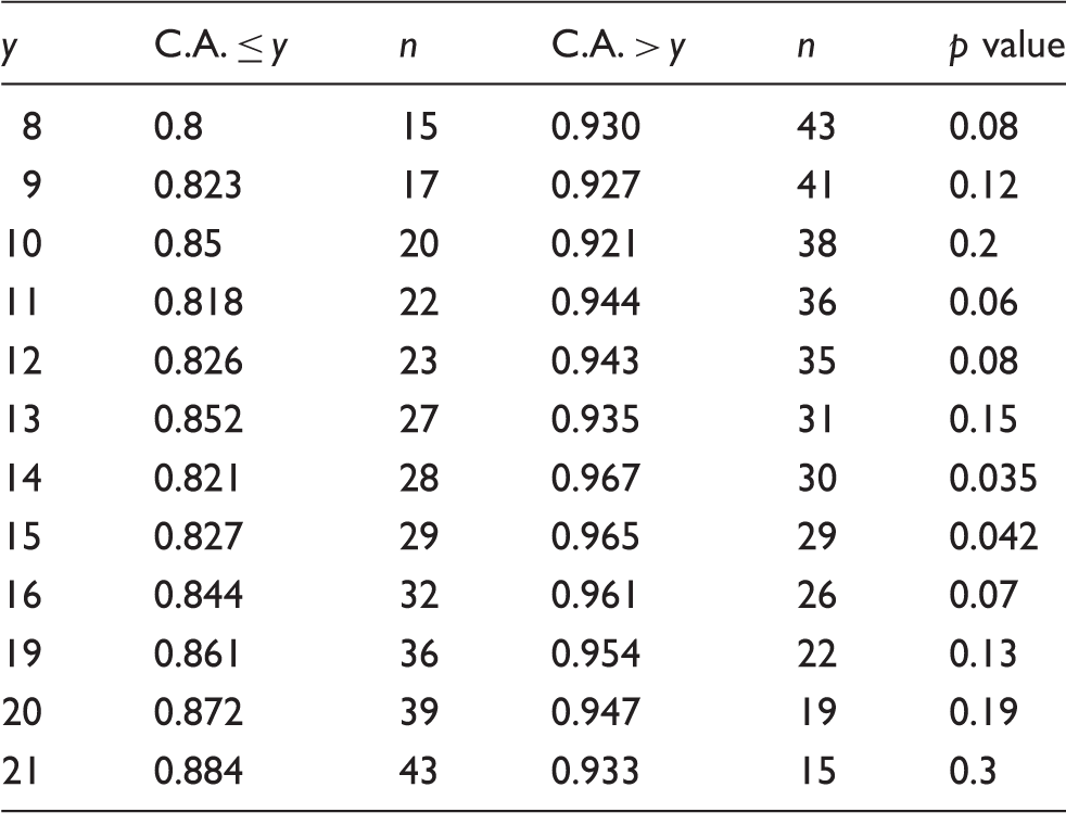
Y: years lived with migraine; C.A. ≤ y: classification accuracy for migraineurs with equal to or less than x number of years lived with migraine; C.A. > y: classification accuracy for migraineurs with more than x number of years lived with migraine; n: number of migraine patients for a specific threshold. p value: classification accuracy differences between subgroups for a specific migraine threshold. Significant classification accuracy differences were shown for the 14 and 15 migraine years threshold subgroups. Example: Significant differences in classification accuracy were found for the threshold of 14 years of migraine (y = 14). Migraine patients who lived with more than 14 years of migraine (n = 30; classification accuracy = 0.967) were significantly better classified (p = 0.035) than migraine patients who lived with 14 years of migraine or less (n = 28; classification accuracy = 0.821).

Results

Two patients were excluded because of incomplete datasets. One migraine patient was excluded because of a scanner-related error during slice acquisition, one control participant was excluded because of an abnormality found on MR structural imaging (enlarged ventricles) that prevented an accurate transformation to a normalized brain template during the rs preprocessing stage, and one control individual was excluded for exceeding the predefined movement threshold in the scanner (>2 mm). Fifty-eight migraine patients (mean age = 36.3 SD = 11.5; 44 female and 14 male) and 50 healthy controls (mean age = 35.9, SD = 11.0; 36 female and 14 male) were included in the final analysis. See Table 3. Fifty-one patients had episodic migraine and seven individuals had chronic migraine. Thirty-four patients had migraine without aura and 24 had migraine with aura. An equal ratio of migraine patients and healthy controls was scanned at each of the two institutions. Fifty-nine individuals (32 migraine patients and 27 healthy controls) were recruited from Washington University, and 49 individuals (26 migraine patients and 23 healthy controls) were recruited from Mayo Clinic Arizona. There were no significant differences between migraine patients and healthy controls on age (p = 0.84), levels of anxiety at the time of testing (State, p = 0.23), and generally felt anxiety (Trait, p = 0.11). Migraineurs reported having on average 7.6 headache days per month and had migraines on average for 16.7 years (see Table 1). Although there were significant group differences in levels of depression between migraine patients and healthy controls (BDI-II; migraine patients: mean = 4.0, SD = 4.1; healthy controls: mean = 2.2, SD = 4.1; p = 0.026), average levels of depression were well within the normal range (no depression) for migraine patients and controls (BDI < 10 = normal levels). Data of 30 migraine patients and 20 healthy controls used in this study were included in a previously published paper by Schwedt et al. (36).

Table 3.

Participant characteristics for migraine patients and healthy controls.

	Migrainen = 58	Controlsn = 50	p value
Age, mean (SD)	36.3 (11.5)	35.9 (11.0)	0.84
Sex (F/M)	44/14	36/14	0.65
BDI-II (SD)	4.0 (4.1)	2.2 (4.1)	0.026 a
STATE (SD)	26.5 (7.1)	25.0 (5.5)	0.23
TRAIT (SD)	31.1 (9.1)	28.4 (8.0)	0.11
Headache frequency, mean (SD)	7.6 (5.3)	N/A	N/A
Years with migraine, mean (SD)	16.7 (10.3)	N/A	N/A
Aura/no aura	24/34	N/A	N/A

F: female; M: male; BDI-II: Beck Depression Inventory (II); STATE: State anxiety inventory; TRAIT: Trait anxiety inventory; Headache frequency: days with headache per month.

a

Although there are significant group differences in BDI raw scores, the average BDI scores for healthy controls and migraine patients are consistent with the absence of depression.

Classification results

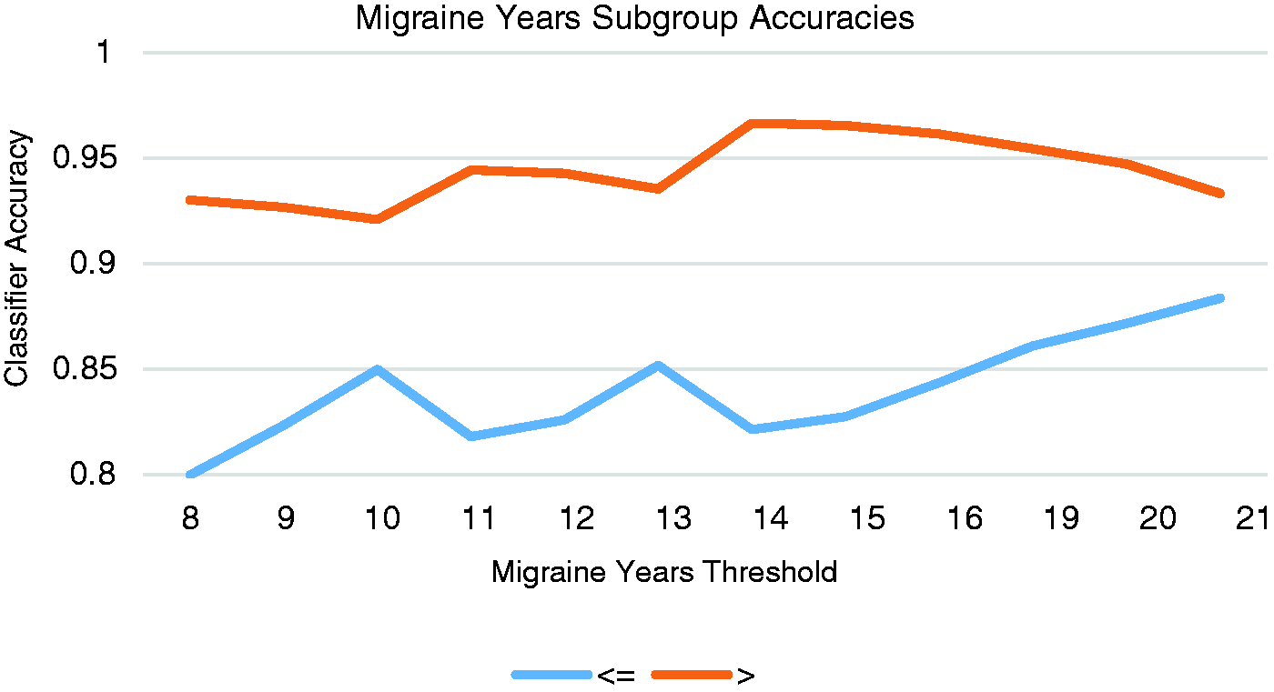
Results indicated an overall accuracy of 81.0% and a best accuracy of 86.1% for classifying individual migraine patients from healthy controls based exclusively on the rs-fc patterns of six ROIs (right middle temporal, right posterior insula, right middle cingulate, bilateral amygdala and left ventromedial prefrontal brain regions). Brain connectivity to the regions that most significantly contributed to the classification accuracy is shown in Figure 2 and Table 4. A post-hoc analysis that interrogated whether the accuracy of the best classifier was associated with migraine burden indicated that migraine patients with longer disease durations were more accurately classified (threshold >14 years; n = 30; classification accuracy = 96.7% and threshold > 15 years; n = 29; classification accuracy = 96.5%) than patients with shorter disease durations (threshold ≤ 14 years; n = 28; classification accuracy = 82.1%. p = 0.035 and threshold ≤ 15 years; n = 29; classification accuracy = 82.7%. p = 0.042). Table 2 shows the classification accuracies of all investigated thresholds and Figure 3 illustrates the classifier accuracy for all migraine years thresholds.

Figure 2.

Functional connectivity patterns of six regions (A–F) that significantly contribute to the classification accuracy of distinguishing between individual migraine patients and healthy controls.

Figure 3.

Classifier accuracy (y axis) for specific migraine years thresholds (x axis). The color “orange” shows the classifier accuracy for migraine patients that were above a specific threshold and the color “blue” shows the classifier accuracy for migraine patients that were equal to or below a specific threshold.

Table 4.

Functional connectivity patterns of six regions (A–F) with important left and right hemisphere areas that contribute to the classification accuracy of distinguishing between individual migraine patients and healthy controls.

R amygdala
X	Y	Z	# voxels	Region	Area
Left
−17	29	39	10	Frontal	Medial frontal
−36	52	6	17	Frontal	Middle frontal
0	−84	12	120	Occipital	Cuneus
−35	−68	5	181	Occipital	Middle occipital
0	−4	−3	6	Subcortical	Hypothalamus
−26	−24	22	640	Subcortical	Insula
−20	−34	3	11	Subcortical	Thalamus pulvinar
−19	−17	9	21	Subcortical	Thalamus VPLN
−25	−42	−21	103	Cerebellum	Anterior
−23	−62	−44	116	Cerebellum	Posterior
Right
8	−6	57	38	Frontal	Medial frontal
36	6	52	12	Frontal	Middle frontal
20	10	53	10	Frontal	Superior frontal
62	−23	8	8	Temporal	Superior temporal
18	−71	48	14	Parietal	Anterior precuneus
39	−56	44	43	Parietal	Inferior parietal lobule
14	−99	−5	7	Occipital	Lingual
10	2	11	82	Subcortical	Caudate body
7	20	33	40	Subcortical	Middle cingulate
25	27	5	9	Subcortical	Claustrum
33	−16	−17	93	Subcortical	Hippocampus
34	24	15	25	Subcortical	Insula
19	−30	−17	15	Cerebellum	Anterior
11	−78	−24	15	Cerebellum	Posterior
1	−22	1	17	Brainstem	Midbrain
L amygdala
X	Y	Z	# voxels	Region	Area
Left
−32	41	30	14	Frontal	Middle frontal
−21	52	28	22	Frontal	Superior frontal
0	−36	69	7	Frontal	Paracentral lobule
−32	−58	46	21	Parietal	Inferior Parietal lobule
−20	−64	34	17	Parietal	Anterior precuneus
−15	−54	65	7	Parietal	Postcentral
−35	−39	34	21	Parietal	Supramarginal
−33	−76	6	22	Occipital	Middle occipital
−19	8	23	388	Subcortical	Caudate body
−27	−37	16	7	Subcortical	Caudate tail
−39	13	14	15	Subcortical	Insula
−27	−15	−35	23	Subcortical	Uncus
−23	−69	−13	12	Cerebellum	Posterior
Right
4	30	42	54	Frontal	Medial frontal
23	1	45	252	Frontal	Middle frontal
27	46	21	27	Frontal	Superior frontal
3	−33	49	64	Frontal	Paracentral lobule
57	−40	−19	21	Temporal	Inferior temporal
32	12	−23	17	Temporal	Superior temporal
19	−16	−12	244	Temporal	Parahippocampal
15	−63	31	13	Parietal	Anterior precuneus
43	−42	48	11	Parietal	Inferior parietal lobule
17	24	24	17	Subcortical	Anterior cingulate
28	−20	26	7	Subcortical	Insula
49	−50	−29	7	Cerebellum	Posterior
R posterior insula
X	Y	Z	# voxels	Region	Area
Left
−33	27	−3	12	Frontal	Inferior frontal
−10	60	7	13	Frontal	Medial frontal
−22	2	43	41	Frontal	Middle frontal
−35	25	35	20	Frontal	Precentral
−5	−49	59	42	Parietal	Anterior precuneus
−28	−70	−11	287	Occipital	Lingual
−21	−6	−22	35	Subcortical	Amygdala
−15	45	−7	20	Subcortical	Anterior cingulate
−18	−40	43	12	Subcortical	Middle cingulate
−35	14	10	9	Subcortical	Insula
Right
28	7	43	44	Frontal	Middle frontal
7	−30	50	12	Frontal	Paracentral lobule
59	−5	7	54	Temporal	Superior temporal
27	−36	−14	95	Temporal	Parahippocampal
26	−33	60	25	Parietal	Postcentral
13	−93	8	12	Occipital	Cuneus
21	−72	−10	48	Occipital	Lingual
31	−2	−23	19	Subcortical	Amygdala
13	28	25	170	Subcortical	Anterior cingulate
16	−7	45	33	Subcortical	Middle cingulate
16	−47	16	406	Subcortical	Posterior cingulate
18	−19	7	9	Subcortical	Thalamus VPLN
25	−8	−41	9	Subcortical	Uncus
8	−54	−20	19	Cerebellum	Anterior
17	−75	−33	67	Cerebellum	Posterior
R middle cingulate
X	Y	Z	# voxels	Region	Area
Left
−35	19	−11	39	Frontal	Inferior frontal
−9	46	16	79	Frontal	Medial frontal
−37	19	26	44	Frontal	Middle frontal
−44	−9	−24	18	Temporal	Anterior fusiform
−30	−53	−1	28	Temporal	Parahippocampal
−45	−36	45	35	Parietal	Inferior parietal lobule
−20	−31	61	17	Parietal	Postcentral
−32	−54	57	7	Parietal	Superior parietal lobule
−5	−68	3	600	Occipital	Lingual
−12	−41	16	11	Subcortical	Posterior cingulate
−29	−29	−5	9	Subcortical	Hippocampus
−40	−19	−6	32	Subcortical	Insula
−16	−6	−24	16	Subcortical	Uncus
right
5	−22	61	16	Frontal	Medial frontal
49	11	38	7	Frontal	Middle frontal
27	55	7	23	Frontal	Superior frontal
3	−41	62	25	Frontal	Paracentral lobule
50	12	0	45	Temporal	Superior temporal
11	−51	56	13	Parietal	Anterior precuneus
41	−45	54	7	Parietal	Inferior parietal lobule
20	−90	−5	13	Occipital	Lingual
11	13	20	515	Subcortical	Caudate body
22	9	34	16	Subcortical	Middle cingulate
33	−18	−7	15	Subcortical	Thalamus LN
7	−10	−32	9	Brainstem	Pons
R middle temporal
X	Y	Z	# voxels	Region	Area
Left
−7	41	39	24	Frontal	Medial frontal
−41	−69	30	14	Temporal	Middle temporal
−40	−55	12	22	Temporal	Superior temporal
−28	−30	49	133	Parietal	Postcentral
−5	−68	9	104	Occipital	Cuneus
−9	41	2	7	Subcortical	Anterior cingulate
−25	−59	11	14	Subcortical	Posterior cingulate
−38	−31	26	36	Subcortical	Insula
−14	−85	−21	33	Cerebellum	Posterior
Right
44	24	−4	26	Frontal	Inferior frontal
15	38	33	117	Frontal	Medial frontal
33	−2	41	78	Frontal	Middle frontal
−41	−69	30	14	Temporal	Middle temporal
33	5	−16	37	Temporal	Superior temporal
12	−57	50	36	Parietal	Anterior precuneus
13	−53	67	7	Parietal	Postcentral
21	−85	18	38	Occipital	Cuneus
3	7	10	108	Subcortical	Caudate body
34	−19	−9	40	Subcortical	Caudate tail
22	47	1	68	Subcortical	Anterior cingulate
11	−54	10	10	Subcortical	Posterior cingulate
24	24	−1	16	Subcortical	Claustrum
9	−14	14	6	Subcortical	Thalamus AN
52	−47	−24	21	Cerebellum	Posterior
−2	−28	−5	9	Brainstem	Midbrain
l VMPFC
X	Y	Z	# voxels	Region	Area
Left
−32	41	19	66	Frontal	Middle frontal
−8	44	40	13	Frontal	Superior frontal
−21	−21	53	36	Frontal	Precentral
−25	−23	−28	27	Temporal	Parahippocampal
−21	v64	36	41	Parietal	Anterior precuneus
−22	−86	0	35	Occipital	Lingual
−26	−59	−5	101	Occipital	Posterior fusiform
−17	24	−10	30	Subcortical	Caudate head
−22	7	49	60	Subcortical	Middle cingulate
−20	3	10	12	Subcortical	Thalamus LN
0	−55	−3	31	Cerebellum	Anterior
−18	−41	−34	24	Cerebellum	Posterior
Right
10	−22	46	15	Frontal	Medial frontal
16	58	22	14	Frontal	Superior frontal
7	18	−19	7	Frontal	Rectal
51	−20	−23	43	Temporal	Anterior fusiform
33	−8	−36	24	Temporal	Inferior temporal
49	0	−28	25	Temporal	Middle temporal
8	−85	21	14	Occipital	Cuneus
16	−50	0	19	Occipital	Lingual
24	−72	21	114	Occipital	Posterior precuneus
29	2	−18	14	Subcortical	Amygdala
5	−3	21	43	Subcortical	Caudate body
33	−12	8	15	Subcortical	Claustrum
23	−65	−33	193	Cerebellum	Posterior

#voxels: number of neighboring voxels in a cluster; LN: lenticular nucleus; VPLN: ventral posterolateral nucleus; AN: anterior nucleus.

X,Y,Z coordinates are labeled in Montreal Neurological Institute (MNI) space.

Discussion

This study investigated the utility of rs-fMRI data to distinguish individual migraine patients from healthy control individuals. Results indicated that rs-fc patterns of pain-processing regions provided good discriminative power for classifying between migraine patients and healthy controls. In addition, this study also demonstrated that migraine patients with longer disease durations were more accurately classified compared to migraine patients with shorter disease durations.

Out of the 33 predefined ROIs, which are known pain-processing areas that mediate cognitive, affective, sensory-discriminative and modulatory components of pain, whole-brain voxel-by-voxel connectivity of six regions (bilateral amygdala, right middle temporal, posterior insula, middle cingulate, and left ventromedial prefrontal brain regions) had the most discriminative power and were found to significantly contribute to the accuracy of discriminating between migraineurs and healthy controls with an overall accuracy of 81.0% and a best accuracy of 86.1%. Interestingly, four out of the six seeded ROIs were lateralized to the right hemisphere (right amygdala, middle temporal, posterior insula and middle cingulate) and the recombinant brain clusters that contributed to each of these ROIs also showed a tendency to involve more right compared to left hemispheric regions. This is in line with data that suggest a right hemispheric dominance in pain processing (28).

Frontal and limbic regions

The involvement of the bilateral amygdala, insula, ventromedial prefrontal cortex and middle cingulate regions is intriguing, as these regions are part of the broader limbic network and are involved in the sensory-discriminative and emotional components of the pain experience (37) including the processing of unpleasant emotions, pain expectation and anxiety toward pain (38–41). Increased middle cingulate and ventromedial prefrontal cortex activation has been demonstrated in healthy controls using positron emission tomography when participants were uncertain whether they would receive a painful stimulus (42) and interictal migraineurs showed stronger middle cingulate activation relative to healthy controls during heat pain processing (10). Stankewitz and May found increased limbic activity in ictal compared to interictal migraineurs during the processing of olfactory stimuli (2). Hadjikhani et al. showed increased functional connectivity between the amygdala and other limbic areas in migraineurs with and without aura relative to healthy controls as well as compared to patients with other chronic pain conditions (5). Maleki et al. showed volume loss and lower functional activation in the insula in high-frequency migraineurs compared with low-frequency migraineurs, potentially indicating that migraine frequency drives structural and functional brain changes (43).

Right middle temporal cortex

Structural and functional changes in the temporal lobe have been well described in migraine (36,44,45) and other headache disorders (46,47). For example, Naegel and colleagues noted gray matter decrease in the right middle temporal lobe in cluster headache patients compared to healthy controls (46), and Schwedt et al. found altered cortical thickness correlations of the right middle temporal lobe with contralateral frontal regions in migraine patients relative to healthy controls (48). Although the temporal lobe has been hypothesized to be involved in central sensitization in migraine (1,36), the precise role of the middle temporal lobe is still debated.

Finally, results showed that migraineurs with longer disease durations were more accurately classified than migraineurs with shorter disease durations, potentially indicating that recurrent migraines over many years might progressively alter the functional connections of pain-processing regions. Henceforth, one might hypothesize that the functional connections of regions that contributed to the classification accuracy identify brain areas that “re-wire” as a result of years lived with recurrent migraines and signify functional connections that track the course or burden of the disease.

There are several limitations: 25 migraine patients reported that they developed a migraine ≤48 hours after the scan. Although all patients reported to be pain free at the time of testing and denied migraine symptoms prior to undergoing imaging, it is possible that some patients might have been in the premonitory phase of migraine. Future studies using larger sample sizes will be needed to determine classification accuracy among those who are within 48 hours of their next migraine versus those who are further out. We estimated brain connectivity for several a priori defined brain regions (33 ROIs) with every voxel in the brain. These regions were selected based on functional imaging findings that have consistently shown these pain-processing areas to undergo functional change in migraine. As we limited our model to interrogating the connectivity of only these 33 ROIs with the rest of the brain, we might have missed other important regions that could have further improved our classification accuracy. Additionally, because of the sample-size limitations we were not able to evaluate classification accuracy for subgroups of migraineurs, i.e. between migraineurs with and without aura or migraineurs with high versus low migraine frequency. Future studies will be necessary to explore the utility of rs-fMRI for the classification of migraine subgroups.

Summary

The present study assessed the utility of a classification algorithm for discriminating between migraineurs and healthy controls based on rs-fMRI data only. Results indicated that fc with the bilateral amygdala, the right middle temporal, right posterior insula and right middle cingulate as well as the left ventromedial prefrontal region could accurately distinguish migraine patients from healthy controls with an overall accuracy of 81.0%. These findings suggest that the functional connections of pain-processing regions are altered in migraineurs, particularly for regions involved with processing the affective components of pain. Migraineurs with longer disease durations were more accurately classified than those with shorter disease durations, suggesting that disease burden might change the functional connections in the brain. The current findings suggest that rs-fMRI has good utility for classifying individual migraine patients and could potentially indicate the applicability of rs-fMRI for identifying disease biomarkers. The aberrant patterns of functional connections that distinguish migraine patients from healthy controls could represent core changes associated with the migraine disease process that are further reformed by recurrent pain. In the future, longitudinal assessments of these functional connections might help to elucidate the course of the disease and could provide insight into identifying individual migraine patients who are likely to recover as well as those individuals who will develop more severe forms of migraine. Additional studies are needed to optimize the classification accuracy (e.g. combining structural and functional imaging data) and to validate the accuracy of the classifier described herein.

Clinical implications

Brain resting-state functional connectivity models allow for the accurate classification of eight out of 10 migraine patients from healthy controls.

Migraine patients with longer disease durations were more accurately defined by functional neuroimaging than migraineurs with shorter disease durations, thus indicating that disease burden might drive functional reorganization.