Sage Journals: Discover world-class research

Abstract

Purpose:

In between migraine attacks, some people show visual field defects that are worse when measured closer to the end of a migraine event. In this cohort study, we consider whether electrophysiological responses correlate with visual field performance at different times post-migraine, and explore evidence for cortical versus retinal origin.

Methods:

Twenty-six non-headache controls and 17 people with migraine performed three types of perimetry (static, flicker and blue-on-yellow) to assess different aspects of visual function at two visits conducted at different durations post-migraine. On the same days, the pattern electroretinogram (PERG) and visual evoked response (PVER) were recorded.

Results:

Migraine participants showed persistent, interictal, localised visual field loss, with greater deficits at the visit nearer to migraine offset. Spatial patterns of visual field defect consistent with retinal and cortical dysfunction were identified. The PERG was normal, whereas the PVER abnormality found did not change with time post-migraine and did not correlate with abnormal visual field performance.

Conclusions:

Dysfunction on clinical tests of vision is common in between migraine attacks; however, the nature of the defect varies between individuals and can change with time. People with migraine show markers of both retinal and/or cortical dysfunction. Abnormal visual field sensitivity does not predict abnormality on electrophysiological testing.

Keywords

Migraine contrast visual fields visual evoked potential electroretinogram

Introduction

Migraine is a common neurological disorder involving vision. Many studies have identified abnormal visual function in between migraine attacks (the interictal period). These include perceptual measures of cortical visual processing (e.g. (1 –4)), as well as electrophysiology (e.g. (5 –14)) and visual field assessment using static (15 –22), flickering (20,23,24), and blue-on-yellow perimetry (25,26).

Previous literature does not suggest a single, common anatomical locus for visual anomalies in migraine. Brain neuroimaging has demonstrated structural changes in both primary visual cortex (V1) and extrastriate areas (for a review, see Schwedt and Dodick (27)). Electrophysiology suggests cortical involvement, as abnormal cortical evoked potentials occur concurrently with normal retinal responses (6,8,14). However, there is also evidence for involvement of the pre-cortical visual pathways. Case studies demonstrate retinal vascular involvement in some individuals (e.g. (28)), and reduced retinal nerve fibre layer thickness (29) and transient retinal vasospasm (30) have been associated with migraine. Several studies report performance differences on psychophysical tasks that assess pre-cortical vision (4,31 –35). Furthermore, the spatial pattern of visual field defects can resemble retinal (e.g. monocular and arcuate (15,18,20,21,23,25,26)) or cortical (e.g. bilateral and homonymous (17,19,22)) dysfunction in different people. These interictal visual field defects do not only occur in people who experience visual aura during their migraine attacks.

A challenge for experiments considering the anatomical locus of visual dysfunction in migraine is the fact that migraine is an episodic condition. Visual function can vary with time – both in the lead up to a migraine (10,36,37) and post-migraine (9,16,19,20,24). The increase (36,37) and normalisation (10) of cortical evoked potentials in the pre-attack period are presumed to reflect physiological changes involved in the build up to a migraine event, such as the normalisation of cortical excitability (38,39) or the increase in serotonin immediately before an attack (37,40). In contrast, visual field defects are worse the day after a migraine (24) and gradually improve over time (16,19,20), which suggests that they may be sequelae of migraine.

In this study, we compare visual fields and electrophysiology in the same individuals, measured on the same day, at different time-points after migraine. To our knowledge, this is the first study to directly compare visual field assessment with electrophysiology in the same migraine cohort. We consider the anatomical locus of abnormalities, as inferred from the spatial pattern and binocularity of visual field defects, and from comparison of simultaneously recorded pattern electroretinogram (PERG) and visual evoked response (PVER).

Methods

Participants

The study was approved by the Human Research Ethics Committee of the University of Melbourne (HREC #0932638). Written informed consent, according to the tenets of the Declaration of Helsinki, was obtained prior to participation.

The study included people with migraine and non-headache controls. Participants were recruited from 75 participants in a previous cross-sectional study (14), who were all asked to return for a second test. After regular follow-up attempts were made by phone and email from June 2010 to July 2012, 17 people with migraine (11 MO, 6 MA) and 26 non-headache controls returned. All participants were screened to satisfy the following inclusion criteria: best corrected visual acuity ≥6/7.5 (logMAR), subjective refraction within ±5.00D sphere and −2.00D astigmatism, intraocular pressure <21 mmHg by Goldmann applanation tonometry, age-normal findings on slitlamp biomicroscopy, ophthalmoscopy and optic nerve head imaging with the Heidelberg Retinal Tomograph (HRT), and no systemic disease or medications known to affect visual function or neurological state, including prophylactive migraine medications. The control (19–46 years) and migraine (19–43 years) groups did not differ in age (Mann Whitney rank sum test, p = 0.12). Neither was there a group difference in global rim area (F(2,71) = 1.08, p = 0.34) or volume (F(2,71) = 0.98, p = 0.38) of the optic nerve head, which are two HRT parameters that correlate with perimetric indices describing generalised and localised visual field loss in people with glaucoma (41).

Participants completed a clinical interview, headache questionnaire and the Migraine Disability Assessment Score (MIDAS) questionnaire (42) to describe their migraine attacks, where applicable (Table 1). The MIDAS questionnaire score measures the number of days in the preceding three months where migraine attacks resulted in reduced productivity in tasks of daily living. Scores are interpreted as minimal (Grade 1, score 0–5), mild (Grade 2, score 6–10), moderate (Grade 3, score 11–20) or severe disability (Grade 4, score 21+). Migraine participants reported symptoms (headache, nausea/vomiting, photophobia, phonophobia) that fulfilled the International Headache Society criteria (43) for migraine without aura (MO) and migraine with aura (MA). The MO and MA groups were pooled, as both groups demonstrate similar visual field losses (16,18,20,21,23 –25). Control participants had never had a migraine and were free from regular headaches (less than four in the past year).

Table 1.

Summary of self-reported migraine characteristics (median, range).

Migraine characteristics
MO	MA	Statistic	p
Days since last migraine at Visit 1	18 (7–150)	25 (7–200)	U = 26.0	0.51
Days since last migraine at Visit 2	3 (1–5)	2 (1–6)	U = 24.0	0.38
Age at first migraine (years)	15 (4–17)	12 (10–30)	U = 21.0	0.24
Years of migraine	13 (3–23)	20 (7–30)	t₁₅ = 0.77	0.45
Migraine attacks in past year	8 (1–50)	5 (1–50)	U = 17.5	0.39
Weeks between migraine attacks	3 (1–20)	6 (1–24)	U = 22.0	0.29
Estimated number of lifetime attacks	100 (30–550)	89 (14–1300)	U = 25.0	0.45
MIDAS questionnaire score (days)	20 (0–49)	3 (1–4)	U = 7.0	0.010
Headache duration (hours)	12 (2–72)	8 (2–48)	U = 26.0	0.51

Independent sample t-tests and Mann Whitney rank sum tests comparing the migraine characteristics between groups are provided.

MIDAS: Migraine Disability Assessment Score; MO: migraine without aura; MA: migraine with aura.

Timing of the test visits

Each session lasted up to three hours. For people with migraine, the first visit was scheduled at least one week post-migraine. The second visit was scheduled as close as practicable, but at least one day, after the cessation of migraine symptoms (maximum six days post-migraine). The difference in the number of days post-migraine between the two visits ranged from three to 199 days (Figure 1; median 16 days). Control participants completed two sessions at least one day apart (median 18 days, range 1–132 days).

Figure 1.

Days since last migraine at the two test visits for the migraine participants. MO participants are shown as filled square symbols, whereas MA participants are shown as filled diamond symbols. The MO participant who was tested one day before a migraine is shown as a cross symbol. Visit 1 was scheduled at least seven days after a migraine. Visit 2 was scheduled at a time closer after a migraine (within six days). MO: migraine without aura; MA: migraine with aura.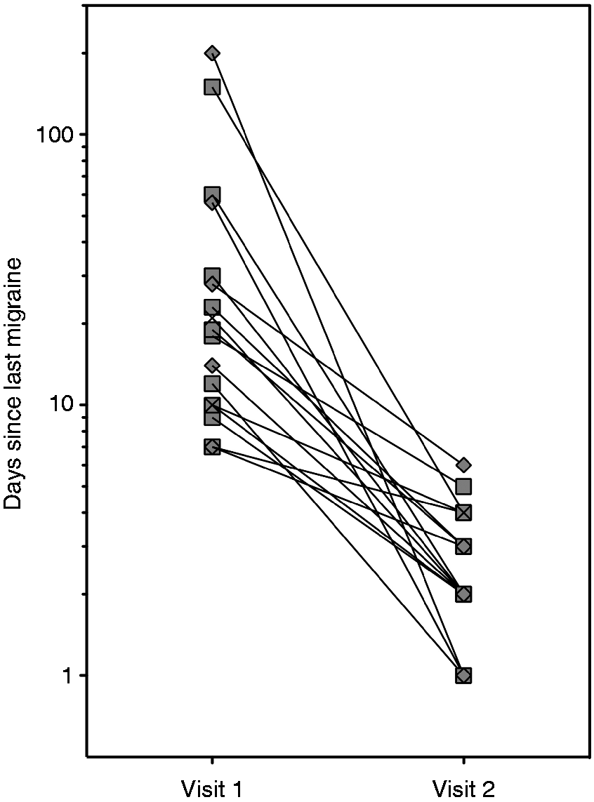

Increased PVER amplitude has been reported in the pre-attack period, up to 72 hours before a migraine (37). Prodromal symptoms, including fatigue and difficulty concentrating, commonly occur up to 48 hours before an attack (44) and may affect a person’s visual field performance. To address this, all participants were contacted (by phone or email) after each test session. This follow-up found that the majority of participants did not have a migraine within 72 hours of each test session. One of the 17 participants experienced a migraine the day after the first test session. Data from this participant have been represented as cross symbols in Figures 1 –3. Excluding the data from this individual from statistical analyses did not change our conclusions.

Figure 2.

PVER amplitudes at the two test visits. (a) Steady-state PVER. (b) Transient PVER. Individual data are presented for the control (unfilled symbols) and migraine (MO: filled squares, MA: filled diamonds) participants. The MO participant who was tested one day before a migraine is shown as a cross symbol. Visit 1 was scheduled at least seven days after a migraine. Visit 2 was scheduled at a time closer after a migraine (within six days). Error bars represent the group mean ± 95% CI of the mean. PVER: pattern visual evoked response; MO: migraine without aura; MA: migraine with aura.

Figure 3.

Global indices of localised visual field loss at the two test visits. (a) SAP Pattern Defect. (b) TMP Pattern Defect. (c) SWAP Loss Variance. Individual data are presented for the control (unfilled symbols) and migraine (MO: filled squares, MA: filled diamonds) participants. The MO participant who was tested one day before a migraine is shown as a cross symbol. Visit 1 was scheduled at least seven days after a migraine. Visit 2 was scheduled at a time closer after a migraine (within six days). Horizontal lines represent the group median. MO: migraine without aura; MA: migraine with aura; SAP: standard automated perimetry; TMP: temporal modulation perimetry; SWAP: short-wavelength automated perimetry.

Visual field tests

Visual field tests were always conducted first because of possible ocular discomfort following electrode placement for PERG recordings. Three different visual field tests were included. Standard automated perimetry (SAP) is the standard perimetric technique and is most commonly encountered in clinical practice. Participants completed SAP first, as it is well tolerated and generally easiest for a naïve observer to learn. Temporal modulation perimetry (TMP) and short-wavelength automated perimetry (SWAP) were conducted next, in random order, as visual field defects in people with migraine have been identified using TMP (20,24) and SWAP (25) that are not measurable on SAP. These different forms of perimetry test different aspects of visual processing, with flicker perimetry preferentially assessing magnocellular pathways (45) and SWAP assessing the blue-on-yellow (or koniocellular) system (46). SAP is non-visual pathway selective (47).

SAP and TMP were performed on the Medmont M-700 perimeter (Medmont Pty Ltd., Camberwell, Victoria, Australia), which has been described elsewhere (48). In brief, the stimuli (λ_max = 565 nm, max luminance 320 cd/m²) are 0.43° (Goldmann size III) light-emitting diodes presented on a background luminance of 3.2 cd/m² (CIE 1931 x = 0.53, y = 0.42) and arranged in concentric rings. SAP thresholds were measured using the Central Threshold test at 103 locations at 1°, 3°, 6°, 10°, 15°, 22° and 30° eccentricities. For TMP, the Auto-Flicker test was conducted at 73 locations at 1°, 3°, 6°, 10°, 15° and 22°. This test varies the temporal frequency of the flickering stimuli with retinal eccentricity (18 Hz, 1°–3°; 16 Hz, 6°; 12 Hz, 10°–15°; 9 Hz, 22°). Stimuli were presented for 200 ms (SAP) and 800 ms (TMP) durations. SWAP was performed on the Octopus 101 perimeter (Haag-Streit Inc., Koeniz, Switzerland), a detailed description of which has been given previously (49). Blue (λ_max = 440 nm) test stimuli of 1.72° (Goldmann size V) were projected for 200 ms against a yellow background (100 cd/m²), to which participants adapted for at least three minutes before testing. Thresholds were measured using the Dynamic strategy (50) at 52 locations at 3°, 9°, 15° and 21° eccentricity.

Participants had a brief practice before testing. Tests with false-positive or false-negative rates above 30% were excluded. The automated blind-spot monitor identified fixation losses exceeding 30% in four control and four migraine participants. However, continuous monitoring of the limbal position by direct visual inspection (Medmont) or via video camera (Octopus) confirmed steady fixation.

Visual field analysis

The global indices generated by the perimeter were analysed. The Medmont perimeter returns Average Defect and Pattern Defect, whereas the Octopus perimeter returns Mean Defect and Loss Variance. These indices are determined relative to a proprietary age-matched normative database and describe generalised and localised visual field loss respectively.

Global indices provide single summary statistics for visual field performance but do not illustrate which locations are abnormal across the visual field. To establish a point-wise assessment of visual field abnormality, we determined two-sided empirical confidence limits of sensitivity at each visual field location (20), based on our 26 control participants. We used our controls because people with migraine are not excluded from the proprietary databases. Locations at and immediately above and below the blindspot were excluded. As visual field outcomes are non-parametric (51), locations where sensitivity was lower than the eighth percentile limit (second worst-performing control) were considered ‘depressed’, and vice versa for ‘better’ points (upper 92nd percentile limit). In the same way, point-wise confidence limits were determined for the change in sensitivity between the first and second visits, where a negative change indicated a reduction in sensitivity at the second visit. Assuming that thresholds at individual locations are independent, visual fields were judged to be abnormally depressed (p < 0.05) if there were at least eight locations below our control group lower limit (p < 0.04 for a single location) out of a total 101 test points on SAP, 6 of 73 on TMP and 5 of 50 on SWAP (see Appendix, Table A1).

The fellow eye was also examined to classify whether the pattern of defect was homonymous. Two approaches were used: (1) visual inspection, to see if locations of depressed sensitivity were in the same hemifield in both eyes and respected the vertical midline; and (2) quadrant analysis (1), where a quadrant was classified as abnormal (p < 0.05) if there were at least four SAP, three TMP or three SWAP locations that were depressed within that quadrant (see Appendix, Table A1). When the same quadrant was classified as abnormal in both eyes, using either criterion, the deficit was considered homonymous.

Pattern electrophysiology

The PERG reflects retinal ganglion cell activity (52), whereas the PVER measures V1 function and integrity of the retinocortical pathway (53) and other brain areas (54). The PERG and PVER were recorded simultaneously to rule out cortical dysfunction arising from the presence of a retinal abnormality. Both ‘transient’ (<3 Hz stimulation) and ‘steady-state’ responses to higher temporal frequency stimulation (≥4 Hz) were included, as visual field sensitivity is worse the day after a migraine when tested with flickering stimuli (TMP) (24). The steady-state response is presumed to share similar neural substrates to behavioural measures of temporal processing (flicker) (55).

The protocol for simultaneous PERG and PVER has been described in detail elsewhere (14). Responses were recorded monocularly according to ISCEV standards (52,53) using the Espion (Diagnosys LLC, Cambridge, UK). Electrode impedance was generally below 5 kOhms and did not exceed 10 kOhms. Participants fixated on a 0.5° diameter red square in the centre of the screen (Sony G520 21-inch CRT monitor: frame rate 100 Hz, resolution 1024 × 786 pixels) positioned 50 cm away. The stimulus was a square-wave checkerboard (31° square field, 52 cd/m² mean luminance, 96% contrast, 0.8° checks), counter-phased at 1 Hz (2 reversals/second, 250 ms epoch, ‘transient’ response) or 8.3 Hz (16.7 reversals/second, 480 ms epoch, ‘steady-state’ response). Stimuli were presented using an interleaved block design to balance the effect of fatigue on recordings.

Two-hundred signals were amplified, bandpass-filtered (1.25–100 Hz), and digitised (1000 Hz) to 16-bit resolution. Timing and amplitude measures were extracted. In compliance with ISCEV standards (52,53), peak times were measured for the positive components of the PERG (P50) and PVER (P100). Peak-to-peak amplitudes were measured for the two neural signals closest in succession along the visual pathway, representing activity of the retinal ganglion cells (PERG P50-N95 amplitude (56)) and V1 (PVER N75-P100 amplitude (54)). The different components were identifiable on all transient waveforms collected. Similarly, the amplitude and phase at the second harmonic (16.7 Hz) of the steady-state PERG and PVER, reflecting retinal ganglion cell (56) and primary visual cortical activity (57), respectively, were determined by Discrete Fourier Transform. Decreased phase values correspond to signal delays in the time domain. Steady-state responses below noise levels at neighbouring frequencies (14.6 and 18.8 Hz) (58) were removed from the dataset. PVER interhemispheric asymmetry (7,9,11,13), which may be related to the laterality of the migraine headache (11) or aura (7,9), was defined as the percentage difference in amplitude between the right and left hemispheres.

Statistical analysis

For control and migraine participants, a worst eye was chosen for analysis based on the total number of abnormal points across all visual fields. Statistical comparisons were performed using SPSS version 20.0 (SPSS Inc., Chicago, IL, United States). Data were tested to confirm statistical normality (Shapiro-Wilk normality test) and homogeneity of variances (Mauchly’s test of sphericity). Repeated-measures analyses of variance considered group differences (RM-ANOVA, α = 0.05) nested within visit (visit 1, 2) and test (transient, steady-state) or perimeter (SAP, TMP, SWAP). Where the assumption of sphericity was violated, the degrees of freedom were amended using a Huynh-Feldt correction. Paired t-tests, or Wilcoxon signed rank tests where the data were non-Gaussian, were used to test for within-individual changes between visits. The alpha level was adjusted using a Holm-Bonferroni correction for multiple comparisons (59).

Results

Changes in electrophysiology with time post-migraine

We find differences in PVER amplitude between migraine and control groups depending on the component analysed (Table 2; group × component interaction: F(1,40) = 7.92, p = 0.008). Separate component analyses indicated reduced steady-state PVER (Figure 2(a); F(1,40) = 11.4, p = 0.002), but normal transient PVER amplitudes (Figure 2(b); F(1,41) = 1.37, p = 0.25) in the migraine group. Our data further demonstrate that PVER amplitude did not change at the second visit; that is, closer to a migraine. Comparisons between the two visits were performed using paired t-tests and none was found to be significant (steady-state: controls t₂₅ = 1.20, p = 0.24, migraine t₁₅ = 1.88, p = 0.079; transient: controls t₂₅ = 1.63, p = 0.12, migraine t₁₆ = 1.58, p = 0.13). Neither was there a significant change in PVER timing (Table 2; group × visit interaction: F(1,40) = 0.95, p = 0.34), PVER/PERG ratio (Table 2; group × visit interaction: F(1,40) = 0.05, p = 0.82), or interhemispheric amplitude asymmetry (Table 3; paired Wilcoxon signed rank tests, p > 0.05) with time post-migraine. Although the PERG is normal in between migraine attacks (6,8,14), differences in the PERG may manifest closer to a migraine. We did not find evidence for such an effect (Table 2; group × visit interactions: p > 0.05).

Table 2.

Summary of retinal (PERG) and cortical (PVER) electrophysiological measures (mean ± standard deviation) at the two test visits.

Control		Migraine
Visit 1	Visit 2	Visit 1	Visit 2	RM-ANOVA group comparisons
PERG amplitude (μ V)
Transient response	10.2 ± 2.63	9.79 ± 2.05	11.6 ± 3.22	10.1 ± 2.21	Group: F(1,41) = 1.01, p = 0.32 Group × component: F(1,41) = 2.76, p = 0.10 Group × visit: F(1,41) = 1.36, p = 0.25
Steady-state response	3.23 ± 0.52	3.28 ± 0.62	3.19 ± 0.96	3.20 ± 0.61
PERG timing
Transient peak time (ms)	51 ± 3	51 ± 2	51 ± 2	51 ± 2	Group: F(1,41) = 0.65, p = 0.43 Group × component: F(1,41) = 0.39, p = 0.54 Group × visit: F(1,41) = 0.21, p = 0.65
Steady-state phase (rads)	6.03 ± 0.22	5.81 ± 0.42	6.01 ± 0.24	5.91 ± 0.30
PVER amplitude ( μ V)
Transient response	11.3 ± 5.04	10.6 ± 5.30	12.9 ± 4.80	13.8 ± 5.11	Group: F(1,40) = 0.15, p = 0.70 Group × component: F(1,40) = 7.92, p = 0.008** Group × visit: F(1,40) = 4.04, p = 0.051
Steady-state response	3.89 ± 1.88	3.72 ± 1.95	2.22 ± 1.37	1.87 ± 0.97
PVER timing
Transient peak time (ms)	103 ± 6	102 ± 6	103 ± 6	102 ± 4	Group: F(1,40) = 0.03, p = 0.87 Group × component: F(1,40) = 0.02, p = 0.90 Group × visit: F(1,40) = 0.95, p = 0.34
Steady-state phase (rads)	7.83 ± 1.11	7.94 ± 1.01	7.78 ± 0.48	7.57 ± 1.19
PVER/PERG ratio
Transient	1.19 ± 0.52	1.12 ± 0.52	1.24 ± 0.60	1.23 ± 0.53	Group: F(1,40) = 1.95, p = 0.17 Group × component: F(1,40) = 11.7, p = 0.001** Group × visit: F(1,40) = 0.05, p = 0.82
Steady-state	1.25 ± 0.63	1.19 ± 0.67	0.74 ± 0.51	0.60 ± 0.48

Visit 1 was scheduled at least seven days after a migraine. Visit 2 was scheduled at a time closer after a migraine (within six days).

RM-ANOVAs comparing the electrophysiological measures between groups are provided.

Denotes significance using Holm-Bonferroni correction for multiple comparisons, starting at p < 0.01.

PERG: pattern electroretinogram; PVER: pattern visual evoked response; RM-ANOVA: repeated-measures analysis of variance.

Table 3.

Summary of PVER amplitude interhemispheric asymmetry (median, range) at the two test visits.

	Control			Migraine
	Visit 1	Visit 2	Paired tests	Visit 1	Visit 2	Paired tests
Transient PVER asymmetry (%)	17 (1–37)	21 (3–62)	Z = −1.18, p = 0.24	16 (2–39)	16 (2–43)	Z = −0.40, p = 0.69
Steady-state PVER asymmetry (%)	15 (2–41)	20 (3–51)	Z = −1.06, p = 0.29	22 (3–60)	26 (3–75)	Z = −0.87, p = 0.38

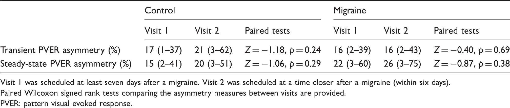
Visit 1 was scheduled at least seven days after a migraine. Visit 2 was scheduled at a time closer after a migraine (within six days).

Paired Wilcoxon signed rank tests comparing the asymmetry measures between visits are provided.

PVER: pattern visual evoked response.

Visual field changes with time post-migraine

For Average/Mean Defect, there was a significant interaction between group, visit and perimeter (Huynh-Feldt ɛ = 0.83, F(1.66,68.1) = 4.02, p = 0.029). The change with time was evident in the control group only – an improvement in SAP Average Defect at the second visit (Table 4; paired t-test: t₂₅ = 4.80, p < 0.001). The migraine participants tended to show worse generalised sensitivity closer to a migraine; that is, a decrease in TMP Average Defect and an increase in SWAP Mean Defect at the second visit. These changes, however, did not reach statistical significance (Table 4; paired t-tests: p > 0.05). The Pattern Defect/Loss Variance is shown in Figure 3 and was similar at both visits for all participants (Table 4; paired Wilcoxon signed rank tests: p > 0.05). Thus, overall, perimetric global indices did not change between visits, although the migraine participants did not show the same learning benefits as controls.

Table 4.

Summary of visual field global indices at the two test visits. (a) Average/Mean Defect (mean ± standard deviation) and (b) Pattern Defect/Loss Variance (median, range).

Control			Migraine
Visit 1	Visit 2	Paired tests	Visit 1	Visit 2	Paired tests
(a) Average/Mean Defect
SAP Average Defect (dB)	−0.85 ± 1.14	−0.04 ± 1.26	t₂₅= 4.80, p < 0.001**	−0.87 ± 1.02	−0.66 ± 1.13	t₁₆= 1.08, p = 0.30
TMP Average Defect (dB)	−3.24 ± 1.04	−3.20 ± 1.09	t₂₅= 0.27, p = 0.79	−3.40 ± 1.23	−3.56 ± 1.17	t₂₅= 0.65, p = 0.52
SWAP Mean Defect (dB)	3.08 ± 2.90	2.92 ± 2.98	t₂₅= 0.77, p = 0.45	3.31 ± 2.85	3.94 ± 2.71	t₂₅= 1.39, p = 0.18
(b) Pattern Defect/Loss Variance
SAP Pattern Defect (dB)	1.44 (0–4.58)	1.67 (0–5.49)	Z = −1.41, p = 0.16	3.14 (0–20.4)	2.02 (0–20.3)	Z = −1.40, p = 0.16
TMP Pattern Defect (dB)	2.30 (0–8.14)	1.57 (0–9.62)	Z = −1.56, p = 0.12	2.25 (0–18.3)	4.26 (0–16.3)	Z = −0.05, p = 0.96
SWAP Loss Variance (dB²)	7.75 (2.20–33.8)	6.35 (2.00–20.5)	Z = −0.92, p = 0.36	13.6 (3.50–113.9)	11.2 (3.70–115.5)	Z = −0.26, p = 0.80

Visit 1 was scheduled at least seven days after a migraine. Visit 2 was scheduled at a time closer after a migraine (within six days).

Paired t-tests and Wilcoxon signed rank tests comparing the global indices between visits are provided.

Denotes significance using Holm-Bonferroni correction for multiple comparisons, p < 0.004.

SAP: standard automated perimetry; TMP: temporal modulation perimetry; SWAP: short-wavelength automated perimetry.

When visual fields of migraine individuals were assessed using point-wise analysis, the majority of locations that were identified as ‘abnormal’ relative to control group performance were depressed, not better (Figure 4, black bars). This was evident for all visual field tasks, although different people were identified as abnormal for each test. The total number of depressed points for a given individual did not change with time post-migraine (Wilcoxon signed rank tests: SAP Z = −0.05, p = 0.96; TMP Z = −0.89, p = 0.38; SWAP Z = −0.32, p = 0.75). However, individuals with migraine showed point-wise changes in sensitivity that fell outside that predicted from control group test–retest variability. The proportion of migraine participants with a significant number of points across the visual field where sensitivity was significantly decreased closer to the end of a migraine was 41% for SAP, 24% for TMP and 47% for SWAP. These proportions were significantly different from controls (chi-square, SAP p = 0.008, TMP p = 0.049, SWAP p = 0.003). In contrast, migraine point-wise sensitivity was not significantly improved at the second visit, when chi-square tests were corrected for multiple comparisons (SAP p = 0.24, TMP p = 0.14, SWAP p = 0.049). To illustrate this, Figure 5 shows the sensitivity at the first visit as a function of sensitivity at the second visit, pooled across the range of visual field locations. Consistent with previous literature (60), both groups showed increased variability for locations with low sensitivity. Whereas, on average, the migraine and control groups showed similar upper limits of test–retest performance, the lower limits of the migraine group were below that of controls across most of the sensitivity range. Thus, people with migraine showed a significant number of points with reduced sensitivity to begin with (Figure 4) and which were associated with larger losses closer to a migraine (Figure 5).

Figure 4.

Proportion of the total number of visual field locations at the first visit (at least seven days after a migraine) that were identified as depressed (black bars) or better (white bars) relative to the lower 8th percentile and upper 92nd percentile limits of control group performance, respectively, for each individual with migraine. The majority of locations identified as abnormal were depressed, not better. A visual field was considered abnormal if there were at least eight SAP, six TMP or five SWAP locations (horizontal dotted lines) that were identified as depressed. Participants in the migraine with aura group (participants 12–17) are shown to the right of each panel. SAP: standard automated perimetry; TMP: temporal modulation perimetry; SWAP: short-wavelength automated perimetry.

Figure 5.

Visual field sensitivity at the second visit plotted as a function of sensitivity at the first visit. The shaded area indicates the 90% CI of test–retest performance for the control group. The 5th and 95th confidence limits for the migraine group are shown as individual symbols. Confidence limits were determined for the range of dB values pooled across all visual field locations. Only sensitivity values appearing at least 20 times were included in the analysis in order to obtain a reasonable estimate of the upper 95% and lower 5% confidence limits. For (a) SAP and (c) SWAP, sensitivity was measured in 1 dB steps, whereas for (b) TMP, sensitivity was measured in 3 dB steps. Consistent with previous literature (60), both groups showed increased variability for locations with low sensitivity. However, the migraine group showed lower limits of visual field sensitivity across the range of sensitivity values. Upper limits were similar between groups. SAP: standard automated perimetry; TMP: temporal modulation perimetry; SWAP: short-wavelength automated perimetry.

Patterns of visual field loss

Where point-wise comparisons revealed a statistically significant number of depressed points, we investigated whether the pattern of visual field loss involved one or both eyes. Data from one migraine participant were excluded from this analysis because of a false negative rate >30% in one eye. Both monocular and bilateral visual field defects were observed in our migraine participants, although the presence of a bilateral defect does not preclude the possibility of two monocular defects.

Only three people with migraine (19%) showed normal results for every visual field task at every visit, compared with 77% controls. Five people with migraine (31%) demonstrated a repeatable bilateral visual field defect (e.g. Figure 6(a)). None gave a homonymous pattern respecting the vertical midline. Nevertheless, as the bilateral visual field loss was diffuse and generalised across the entire field, the majority of cases (80%) satisfied our less conservative definition for homonymous deficits, where at least one quadrant was flagged as ‘abnormal’ in both eyes. On the other hand, four different migraine participants (25%) showed monocular sensitivity loss affecting the same eye at both visits. A further three people (19%) showed normal fields at the first visit, but developed a monocular field defect closer to a migraine (e.g. Figure 6(b)). Monocular defects ranged from patchy loss affecting all four quadrants of a single eye, to an arcuate scotoma that crossed the vertical midline. We interpret these as being of retinal origin.

Figure 6.

Example SAP visual field defects based on point-wise comparisons with control group performance. Shaded squares indicate depressed points; that is, locations where the sensitivity fell below the lower 8th percentile of control group sensitivity. A SAP visual field was considered abnormal if there were at least eight locations across the visual field that were identified as depressed. (a) Diffuse visual field loss in both eyes of a 20-year-old female with migraine with aura. (b) Right eye visual field defect in a 36-year-old female with migraine with aura, showing monocular inferior arcuate loss one day after migraine (left-hand side). Her visual fields were normal at the first visit 56 days after migraine (right-hand side). SAP: standard automated perimetry.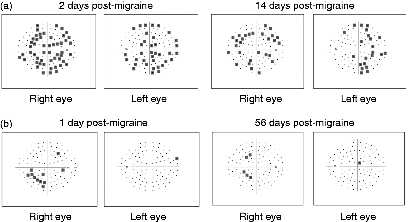

Relationship between abnormal interictal measures of visual function and migraine characteristics

Of the visual field and electrophysiological measures analysed in this study, the steady-state PVER amplitude (Figure 2(a)), Pattern Defect/Loss Variance (Figure 3) and the number of depressed points based on point-wise comparisons (Figure 4) remained consistently abnormal during the post-migraine period. Spearman rank correlations between these measures, averaged across both visits, were not significant (Table 5), implying that these abnormalities might be caused by different mechanisms. To explore the possibility that abnormal interictal measures on electrophysiological or visual field tests related to a particular feature of migraine, correlation coefficients were determined between the consistently abnormal visual functional measures noted above and the migraine characteristics shown in Table 1. None of the correlations was significant (see Appendix, Table A2).

Table 5.

Relationship between steady-state PVER amplitude and visual field measures averaged across both visits.

		R_s	p
SAP	Pattern defect	−0.33	0.19
Depressed points	−0.18	0.48
TMP	Pattern defect	0.07	0.80
Depressed points	0.05	0.84
SWAP	Loss variance	−0.28	0.27
Depressed points	−0.19	0.45

Spearman rank correlations were not significant using a Holm-Bonferroni correction for multiple comparisons, starting at p < 0.008.

PVER: pattern visual evoked response; SAP: standard automated perimetry; TMP: temporal modulation perimetry; SWAP: short-wavelength automated perimetry.

Discussion

The results of this study are consistent with both retinal and cortical visual dysfunction being present in people with migraine. On the one hand, our electrophysiological results, like others (6,8,14), argue for a predominant cortical anomaly in migraine. Steady-state PVER amplitudes were consistently reduced (Figure 2(a)), whereas the PERG was normal, implying no diffuse retinal dysfunction (Table 2). On the other hand, both binocular and monocular visual field defects were found (Figure 6). Monocular patterns of visual field loss arise from pre-chiasmal or retinal dysfunction. The homonymous nature of migraine visual aura and the nature of some bilateral field loss are supportive of a cortical origin. Thus, visual field tests suggest the presence of both cortical and retinal dysfunction in people with migraine. Our findings suggest that the retinal defects affect small, localised regions, whereas the cortical defects tend to involve larger and more generalised regions.

A novel component of this study was the measurement of SAP, TMP and SWAP visual fields as well as transient and steady-state electrophysiological responses on the same day, which enables comparison between these approaches for measuring visual processing in the same individuals. People with migraine show reduced visual field sensitivity to a range of different stimuli, which is consistent with other psychophysical evidence that deficits in people with migraine are not neural pathway-specific (20,24,25,31,33). On the other hand, the steady-state but not transient response at V1 was abnormal in the migraine group. Faster flickering stimuli have consistently demonstrated differences in electrophysiological studies of people with migraine (5,9,61). In some cases, as observed here, a clear separation between migraine and control groups was only measurable in the steady-state response (14,61). Flicker is known to induce higher metabolic demands and increase blood flow in the brain (62). Disrupted neurovascular coupling in migraine (63) may lead to functional abnormalities that depend on flicker rate. The stimulation rate used in the present study (∼8 Hz) corresponds to the temporal frequency that produces a maximal change in cerebrovascular response to a flickering checkerboard pattern as measured by fMRI-BOLD (64). Alternatively, the reduction in steady-state PVER amplitude may reflect abnormal visual motion processing, as the major sources of the steady-state PVER are cortical areas V1 and V5/MT (57). Indeed, there is converging evidence for altered function in visual motion processing pathways from studies involving transcranial magnetic stimulation (65), structural brain imaging (66) and behavioural measures of global motion integration processing (1 –3).

Consistent with earlier reports (16,19,20,22,24), this study demonstrates visual field changes with time post-migraine. However, in this study, sensitivity changes were observed with point-wise comparisons and not by comparing the perimetric global indices. The Pattern Defect/Loss Variance was consistently abnormal, with some migraine individuals showing markedly abnormal values at both visits (Figure 2). It may be that our participants were not tested close enough to a migraine to detect a difference with time. Participants in the previous study were tested the day following migraine offset, with test sessions lasting no more than one hour (24). Our participants, however, were asked to return within one week of a migraine, as we anticipated that it would be more difficult for participants to arrange a second visit of three hours duration at short notice. As a result, the average time post-migraine at the second visit was not 24 hours, but three days. The more demanding nature of the long test session likely biased the timing of the second visit to a day further away from a headache, and prevented migraine participants from completing the second session the day after an attack, where performance is likely to be worse.

A significant number of locations showed a more pronounced reduction in sensitivity one to six days after a migraine. The decrease in sensitivity was not a result of increased variability, as the upper limits of test–retest performance in both groups indicate a similar number and degree of relatively improving locations (Figure 5), consistent with a previous report (24). Differences in visual field sensitivity immediately post-migraine are possibly explained by fatigue or poor concentration as a result of anti-migraine medications or the symptoms of migraine itself. We endeavoured to minimise post-migraine effects by scheduling test visits at least one day after the offset, and not onset, of all migraine symptoms. Moreover, the changes in sensitivity were apparent for discrete locations across the visual field, whereas fatigue would be expected to produce an overall reduction in sensitivity. Differences in Average/Mean Defect in the migraine group did not fall outside the test–retest variability of control group performance (Table 2). An alternative reason for reduced sensitivity is aversion to the test stimuli (67). This might also explain the reduction in steady-state PVER amplitude. We did not formally measure aversion; however, none of the participants reported discomfort or voluntarily withdrew from the study during testing. Furthermore, participants with a strong aversion to visual stimuli are likely to have excluded themselves from volunteering for a study that explicitly involved extensive visual testing.

Although the mechanism for localised visual field deficits in migraine cannot be ascertained from this study, it has been suggested that decreased sensitivity might result from localised vascular events (68). Abnormal peripheral vascular flow and vasospastic tendencies in people with migraine (69,70), particularly transient retinal vasospasms occurring during a migraine attack (30), could cause altered perfusion and increase the risk of focal ischaemic damage to the optic nerve head (68,70) and retina (28). However, the steady-state (flicker) PERG was normal in our migraine group and did not correlate with localised visual field losses. It is worth noting that the pattern electrophysiological measures used in this study involve a large, full-field target and are therefore global responses, which are not designed to find small localised losses or investigate the spatial extent of visual dysfunction. Future studies may take advantage of multifocal techniques (71), which have the potential to provide more information about localised visual field defects. Current multifocal techniques, however, do not have the same spatial resolution as the visual field tests employed in this study, which identify sensitivity losses in people with migraine at discrete locations using test stimuli of 0.5° and 1.7°, although deficits in the peripheral visual field have also been found in people with migraine using larger targets of 10° (1).

We found that an abnormal electrophysiological response did not correlate with visual field performance measured in the same individuals. The difference between electrophysiological and visual field tests may be related to the spatial extent of the test targets, as discussed earlier. In addition, for the most part, electrophysiological measures obtained at least seven days post-migraine were not significantly different from responses obtained, on average, two to three days after an attack, which is consistent with other PVER studies in migraine (10,37). In contrast, visual field sensitivity was worse closer to a migraine, as has been previously reported (16,19,20,24). Without having measured visual function at multiple times in the migraine cycle (i.e. before, during and after an attack), our interpretation of the literature to date is that some visual field defects represent adverse sequelae of migraine, as they are worst in the days following an attack. The effects of migraine can extend from the central nervous system to peripheral organs (e.g. to the retina), which may explain individual cases of ocular involvement in migraine (e.g. (28)) and the development of monocular visual field loss closer to a migraine (e.g. Figure 6(b)). Such retinal changes do not manifest as group differences in the PERG, but are detected by visual field tests that allow spatial localisation. However, abnormal cortical electrophysiological responses are generally unchanged after a migraine, but have been reported to differ before and during an attack (10,36,37). This suggests that changes in neural activity identified using electrophysiology are related to cortical susceptibility to migraine attacks, given that the pathogenesis of migraine involves the brain (27) and the symptomatology of migraine is largely cortical.

The test–retest results of this study also have implications for clinical and research settings where perimetric and electrophysiological techniques are used. Knowing whether deficits are likely to remain stable over time, or are a temporary consequence of migraine, is important for interpretation of test results. The potential for change in visual function after migraine should be considered, as this will affect the ability to determine abnormality and disease progression in people with migraine in comparison with normal test–retest variability.

Clinical implications

We show that both cortical and retinal dysfunction can occur in people who have migraine attacks. In some cases, these appear independent of each other, with visual field changes that appear retinal in origin being variable as a function of time post-migraine.

An abnormal result on an electrophysiological test does not predict whether visual field performance will also be abnormal in people with migraine.

Footnotes

Funding

This work was supported by the National Health and Medical Research Council [grant number 509208] and Australian Research Council [grant number FT0990930] to author AMM. BN was supported by the Elizabeth and Vernon Puzey Postgraduate Scholarship from the Faculty of Science at the University of Melbourne.

Conflict of interest

None declared.

Appendix

References

McKendrick

Badcock

. Motion processing deficits in migraine. Cephalalgia 2004; 24: 363–372.

Antal

Temme

Nitsche

. Altered motion perception in migraineurs: Evidence for interictal cortical hyperexcitability. Cephalalgia 2005; 25: 788–794.

Ditchfield

McKendrick

Badcock

. Processing of global form and motion in migraineurs. Vision Res 2006; 46: 141–148.

Shepherd

Beaumont

Hine

. Motion processing deficits in migraine are related to contrast sensitivity. Cephalalgia 2012; 32: 554–570.

Diener

Scholz

Dichgans

. Central effects of drugs used in migraine prophylaxis evaluated by visual evoked potentials. Ann Neurol 1989; 25: 125–130.

Khalil NM. Investigations of visual function in migraine by visual evoked potentials and visual psychophysical tests. PhD Thesis, University of London, UK, 1991.

Tagliati

Sabbadini

Bernardi

Silvestrini

. Multichannel visual evoked potentials in migraine. Electroencephalogr Clin Neurophysiol 1995; 96: 1–5.

Shibata

Osawa

Iwata

. Simultaneous recording of pattern reversal electroretinograms and visual evoked potentials in migraine. Cephalalgia 1997; 17: 742–747.

Shibata

Osawa

Iwata

. Pattern reversal visual evoked potentials in migraine with aura and migraine aura without headache. Cephalalgia 1998; 18: 319–323.

10.

Judit

Sandor

Schoenen

. Habituation of visual and intensity dependence of auditory evoked cortical potentials tends to normalize just before and during the migraine attack. Cephalalgia 2000; 20: 714–719.

11.

Logi

Bonfiglio

Orlandi

. Asymmetric scalp distribution of pattern visual evoked potentials during interictal phases in migraine. Acta Neurol Scand 2001; 104: 301–307.

12.

Ambrosini

de Noordhout

Sandor

Schoenen

. Electrophysiological studies in migraine: A comprehensive review of their interest and limitations. Cephalalgia 2003; 23: 13–31.

13.

Coppola

Parisi

Fiermonte

. Asymmetric distribution of visual evoked potentials in patients with migraine with aura during the interictal phase. Eur J Ophthalmol 2007; 17: 828–835.

14.

Nguyen

McKendrick

Vingrys

. Simultaneous retinal and cortical visually evoked electrophysiological responses in between migraine attacks. Cephalalgia 2012; 32: 896–907.

15.

Lewis

Vijayan

Watson

. Visual field loss in migraine. Ophthalmology 1989; 96: 321–326.

16.

Drummond

Anderson

. Visual field loss after attacks of migraine with aura. Cephalalgia 1992; 12: 349–352.

17.

Wakakura

Ichibe

. Permanent homonymous hemianopias following migraine. J Clin Neuroophthalmol 1992; 12: 198–202.

18.

De Natale RD, Polimeni D, Narbone MC, et al. Visual field defects in migraine patients. In: Mills RP (ed) Perimetry Update 1992/93 Proceedings of the Xth International Perimetric Society Meeting. Amsterdam/New York: Kugler Publications, 1993, pp. 283–284.

19.

Sullivan-Mee

Bowman

. Migraine-related visual-field loss with prolonged recovery. J Am Optom Assoc 1997; 68: 377–388.

20.

McKendrick

Vingrys

Badcock

Heywood

. Visual field losses in subjects with migraine headaches. Invest Ophthalmol Vis Sci 2000; 41: 1239–1247.

21.

Çomoğlu

Yarangümeli

Köz

. Glaucomatous visual field defects in patients with migraine. J Neurol 2003; 250: 201–206.

22.

Goodwin

. Transient complete homonymous hemianopia associated with migraine. Optometry 2011; 82: 298–305.

23.

McKendrick

Badcock

. An analysis of the factors associated with visual field deficits measured with flickering stimuli in-between migraine. Cephalalgia 2004; 24: 389–397.

24.

McKendrick

Badcock

. Decreased visual field sensitivity measured 1 day, then 1 week, after migraine. Invest Ophthalmol Vis Sci 2004; 45: 1061–1070.

25.

McKendrick

Cioffi

Johnson

. Short-wavelength sensitivity deficits in patients with migraine. Arch Ophthalmol 2002; 120: 154–161.

26.

Yenice

Temel

Incili

Tuncer

. Short-wavelength automated perimetry in patients with migraine. Graefes Arch Clin Exp Ophthalmol 2006; 244: 589–595.

27.

Schwedt

Dodick

. Advanced neuroimaging of migraine. Lancet Neurol 2009; 8: 560–568.

28.

Gutteridge

McDonald

Plenderleith

. Branch retinal artery occlusion during a migraine attack. Clin Exp Optom 2007; 90: 371–375.

29.

Martinez

Proupim

Sanchez

. Retinal nerve fibre layer thickness measurements using optical coherence tomography in migraine patients. Br J Ophthalmol 2008; 92: 1069–1075.

30.

Killer

Forrer

Flammer

. Retinal vasospasm during an attack of migraine. Retina 2003; 23: 253–254.

31.

Coleston

Chronicle

Ruddock

Kennard

. Precortical dysfunction of spatial and temporal visual processing in migraine. J Neurol Neurosurg Psych 1994; 57: 1208–1211.

32.

McKendrick

Vingrys

Badcock

Heywood

. Visual dysfunction between migraine events. Invest Ophthalmol Vis Sci 2001; 42: 626–633.

33.

McKendrick

Badcock

. Contrast-processing dysfunction in both magnocellular and parvocellular pathways in migraineurs with or without aura. Invest Ophthalmol Vis Sci 2003; 44: 442–448.

34.

Tibber

Shepherd

. Transient tritanopia in migraine: Evidence for a large-field retinal abnormality in blue-yellow opponent pathways. Invest Ophthalmol Vis Sci 2006; 47: 5125–5131.

35.

McKendrick

Sampson

. Low spatial frequency contrast sensitivity deficits in migraine are not visual pathway selective. Cephalalgia 2009; 29: 539–549.

36.

Sand

Vingen

. Visual, long-latency auditory and brainstem auditory evoked potentials in migraine: Relation to pattern size, stimulus intensity, sound and light discomfort thresholds and pre-attack state. Cephalalgia 2000; 20: 804–820.

37.

Sand

Zhitniy

White

Stovner

. Visual evoked potential latency, amplitude and habituation in migraine: A longitudinal study. Clin Neurophysiol 2008; 119: 1020–1027.

38.

Siniatchkin

Reich

Shepherd

. Peri-ictal changes of cortical excitability in children suffering from migraine without aura. Pain 2009; 147: 132–140.

39.

Chen

Wang

Fuh

. Peri-ictal normalization of visual cortex excitability in migraine: An MEG study. Cephalalgia 2009; 29: 1202–1211.

40.

Sakai

Dobson

Diksic

. Sumatriptan normalizes the migraine attack-related increase in brain serotonin synthesis. Neurology 2008; 70: 431–439.

41.

Iester

Mikelberg

Courtright

Drance

. Correlation between the visual field indices and Heidelberg retina tomograph parameters. J Glaucoma 1997; 6: 78–82.

42.

Lipton

Stewart

Sawyer

Edmeads

. Clinical utility of an instrument assessing migraine disability: The Migraine Disability Assessment (MIDAS) questionnaire. Headache 2001; 41: 854–861.

43.

International Headache Society . The international classification of headache disorders (2nd edition). Cephalalgia 2004; 24: 9–160.

44.

Blau

. Migraine prodromes separated from the aura: Complete migraine. BMJ 1980; 281: 658–660.

45.

Vingrys A, Demirel S and Kalloniatis M. Multi-dimensional color, flicker and increment perimetry. In: Mills RP and Wall M (eds) Perimetry Update 1994/95 Proceedings of the XIth International Perimetric Society Meeting. Amsterdam/New York: Kugler Publications, 1994, pp. 159–166.

46.

Demirel

Johnson

. Isolation of short-wavelength sensitive mechanisms in normal and glaucomatous visual field regions. J Glaucoma 2000; 9: 63–73.

47.

Swanson

Sun

Lee

Cao

. Responses of primate retinal ganglion cells to perimetric stimuli. Invest Ophthalmol Vis Sci 2011; 52: 764–771.

48.

Vingrys

Helfrich

. The Opticom M-600: A new LED automated perimeter. Clin Exp Optom 1990; 73: 3–17.

49.

Hermann

Paetzold

Vonthein

. Age-dependent normative values for differential luminance sensitivity in automated static perimetry using the Octopus 101. Acta Ophthalmol 2008; 86: 446–455.

50.

Weber

Klimaschka

. Test time and efficiency of the dynamic strategy in glaucoma perimetry. Ger J Ophthalmol 1995; 4: 25–31.

51.

Vingrys

Pianta

. Developing a clinical probability density function for automated perimetry. Aust N Z J Ophthalmol 1998; 26: S101–S103.

52.

Bach

Brigell

Hawlina

. ISCEV standard for clinical pattern electroretinography (PERG): 2012 update. Doc Ophthalmol 2013; 126: 1–7.

53.

Odom

Bach

Brigell

. ISCEV standard for clinical visual evoked potentials. Doc Ophthalmol 2010; 120: 111–119.

54.

Di Russo

Pitzalis

Spitoni

. Identification of the neural sources of the pattern-reversal VEP. Neuroimage 2005; 24: 874–886.

55.

King-Smith

Kulikowski

. Pattern and flicker detection analysed by subthreshold summation. J Physiol 1975; 249: 519–548.

56.

Luo

Frishman

. Retinal pathway origins of the pattern electroretinogram (PERG). Invest Ophthalmol Vis Sci 2011; 52: 8571–8584.

57.

Di Russo

Pitzalis

Aprile

. Spatiotemporal analysis of the cortical sources of the steady-state visual evoked potential. Hum Brain Mapp 2007; 28: 323–334.

58.

Meigen

Bach

. On the statistical significance of electrophysiological steady-state responses. Doc Ophthalmol 1999; 98: 207–232.

59.

Holm

. A simple sequentially rejective multiple test procedure. Scand J Stat 1979; 6: 65–70.

60.

Artes

Iwase

Ohno

. Properties of perimetric threshold estimates from Full Threshold, SITA Standard, and SITA Fast strategies. Invest Ophthalmol Vis Sci 2002; 43: 2654–2659.

61.

Marrelli

Tozzi

Porto

. Spectral analysis of visual potentials evoked by pattern-reversal checkerboard in juvenile patients with headache. Headache 2001; 41: 792–797.

62.

Pastor

Artieda

Arbizu

. Human cerebral activation during steady-state visual-evoked responses. J Neurosci 2003; 23: 11621–11627.

63.

Zaletel

Strucl

Bajrovic

Pogacnik

. Coupling between visual evoked cerebral blood flow velocity responses and visual evoked potentials in migraneurs. Cephalalgia 2005; 25: 567–574.

64.

Singh

Kim

. Correlation between BOLD-fMRI and EEG signal changes in response to visual stimulus frequency in humans. Magn Reson Med 2003; 49: 108–114.

65.

Battelli

Black

Wray

. Transcranial magnetic stimulation of visual area V5 in migraine. Neurology 2002; 58: 1066–1069.

66.

Granziera

DaSilva

Snyder

. Anatomical alterations of the visual motion processing network in migraine with and without aura. PLoS Med 2006; 3: e402–e402.

67.

Marcus

Soso

. Migraine and stripe-induced visual discomfort. Arch Neurol 1989; 46: 1129–1132.

68.

Flammer

Pache

Resink

. Vasospasm, its role in the pathogenesis of diseases with particular reference to the eye. Prog Retin Eye Res 2001; 20: 319–349.

69.

Zahavi

Chagnac

Hering

. Prevalence of Raynaud's phenomenon in patients with migraine. Arch Intern Med 1984; 144: 742–744.

70.

Gasser

Meienberg

. Finger microcirculation in classical migraine. A video-microscopic study of nailfold capillaries. Eur Neurol 1991; 31: 168–171.

71.

Hood

Bach

Brigell

. ISCEV standard for clinical multifocal electroretinography (mfERG) (2011 edition). Doc Ophthalmol 2012; 124: 1–13.

The effect of duration post-migraine on visual electrophysiology and visual field performance in people with migraine

Abstract

Purpose:

Methods:

Results:

Conclusions:

Keywords

Introduction

Methods

Participants

Timing of the test visits

Visual field tests

Visual field analysis

Pattern electrophysiology

Statistical analysis

Results

Changes in electrophysiology with time post-migraine

Visual field changes with time post-migraine

Patterns of visual field loss

Relationship between abnormal interictal measures of visual function and migraine characteristics

Discussion

Clinical implications

Footnotes

Funding

Conflict of interest

Appendix

References