Sage Journals: Discover world-class research

Abstract

Loss of specific human capital is often identified as a mechanism through which displaced workers might experience permanent drops in earnings after job loss. Research has shown that displaced workers who migrate out of their region of origin have lower earnings than those who do not. This paper extends the discussion on returns to migration by accounting for the type of jobs people get and how related they are to their skills. Using an endogenous treatment model to control for selection bias in migration and career change, we compare displaced stayers with displaced movers in Sweden. Results show that migrants who get a job that matches their occupation- and industry-specific skills display the highest earnings among all displaced workers. If migration is combined with a job mismatch, earning losses are instead observed. This group experiences the lowest earnings among all displaced workers.

Keywords

Inter-regional migration specific human capital job match skill relatedness displaced workers

Introduction

Workers who lose their jobs due to firm closure may experience persistent earning losses (Couch and Placzek, 2010; Eliason and Storrie, 2006; Jacobson et al., 1993). One mechanism to cause this is the loss of specific, non-transferable human capital (Becker, 1962). Depending on how similar the new employment is to the previous one, the displaced workers will use their skills and knowledge to different degrees. Research has therefore focused on the importance of industry-specific human capital (Neal, 1995; Neffke et al., 2018; Ong and Mar, 1992), or occupation-specific human capital (Carrington, 1993; Kambourov and Manovskii, 2009; Poletaev and Robinson, 2008; Robinson, 2018) for post-displacement earnings.

Why displaced workers do not find a suitable job related to their occupation- and industry-specific skills can be due to the restricted geography of their job search. If workers look for employment in a larger geographical scale, the probability of getting a good match can be higher (Fackler and Rippe, 2017). This makes relevant the question whether spatial mobility can mitigate the earning losses of displaced workers. Economic theory suggests positive returns to migration where individuals migrate to maximize their expected future income (Sjaastad, 1962), all else equal. However, some studies find that on average, displaced workers who migrate have lower earnings than the ones who do not (Fackler and Rippe, 2017; Huttunen et al., 2018).

The paper aims to expand the discussion on returns to migration for displaced workers by adding one potential mechanism into the equation, namely job-matching. Previous literature has shown that migrants, in general, are more likely to switch industries and occupations than stayers (Greenwood, 1975; Ritchey, 1976). Studies also conclude that migrants who do change occupation or industry experience negative wage returns (Abreu et al., 2015; Krieg, 1997).

While specific human capital is often mentioned as a mechanism behind the earning drop after job loss, this insight has not been combined with the literature on returns to migration after displacement. There are a few papers that do control for job (mis)match when estimating returns to migration, but they focus either only on industrial switches (Abreu et al., 2015) or occupational switches (Krieg, 1997). We argue that both should be considered in measuring returns to migration, as human capital is both industry- and occupation-specific (Sullivan, 2010). Using treatment effects estimations and employing skill-relatedness measures (Neffke and Henning, 2013), our study on Sweden shows that migrants experience higher earnings than stayers when they get employed in a job that matches their industry and occupation skills, but not otherwise. Those who migrate and get an unrelated employment display instead the lowest earnings.

The paper is organized as follows. Returns to migration and job (mis)match section outlines the literature on returns to migration combined with industrial and occupational mobility. Data, method, and variables section introduces the empirical study on Sweden by presenting the matched employer-employee dataset, the identification and empirical design, as well as the variables and descriptive statistics. Results and analysis section shows the empirical findings, and Concluding remarks section concludes.

Returns to migration and job (mis)match

Economic theory treats migration as a choice to maximize expected lifetime income. Sjaastad (1962) argues that migration is an investment in human capital: individuals will migrate if the expected benefits will exceed its costs. According to the Borjas-Roy model (Borjas, 1987; Roy, 1951), workers move to regions where they get more compensation for their skills, no matter if they come from the high or low end of the skill distribution. Standard inter-regional migration models assume therefore that individuals migrate to urban regions to look for better economic opportunities as well as higher expected income (Basile and Lim, 2017; Greenwood, 1985; Herzog et al., 1993; Isserman et al., 1987; Korpi et al., 2010).

However, the empirical literature on returns to migration is split. Some studies find positive returns (Böheim and Taylor, 2007; Dostie and Léger, 2009; Nakosteen and Westerlund, 2004; Yankow, 2003), others find no returns (Axelsson and Westerlund, 1998), and still others prove negative returns, especially after controlling for the self-selection of workers into migration (Pekkala and Tervo, 2002; Smits, 2001; Venhorst and Cörvers, 2018). For displaced workers specifically, the literature leans more towards the fact that there are no returns or negative returns to migration. Huttunen et al. (2018) argue that moves after displacement are not always driven by employment opportunities but rather by family ties. Those who move to smaller regions or where they have family, experience more wage losses than stayers and moves upwards in the urban hierarchy are associated with higher earnings. The latter is in line with the urban wage premium literature that is applicable to the general population and therefore may also apply to displaced workers (Glaeser and Mare, 2001). Fackler and Rippe (2017) show that all displaced workers experience long-lasting earning losses, but movers have worse outcomes than stayers. Boman (2011) suggests that in the short run, migration affects wages negatively, but this effect disappears after 5–6 years.

Venhorst and Cörvers (2018) discuss that one reason for the heterogeneity of findings can be the different mechanisms driving inter-regional migration. For example, Thurow (1975) predicts that employers have information on the quality of regional labor and they, therefore, employ the best workers. The less qualified ones are then pushed out of the labor market. These individuals therefore might be forced to migrate because the alternative would be unemployment in the region of origin. This is what Smits (2001) also puts forward as a reason why there are negative returns to migration for married couples in the Netherlands.

Yet another reason for the heterogeneity of findings can be job match. Inter-regional migration is often associated with a change in industries, occupations, or both (Greenwood, 1975; Ritchey, 1976). Gallaway (1969) was the first to argue that when examining returns to migration, there is a selection bias where industrially mobile individuals are different from the ones who are immobile, something that affects their later earnings. When this industrial switch is accounted for, migrants earn more than stayers. Shaw (1991) shows that workers with high industry- and occupation-specific skills find it advantageous to move to another region for better wages, but this wage growth dampens if the migration is followed by an industry change. Similarly, Krieg (1997) focuses on occupational mobility and discusses that simultaneous changes in location and occupation harm wages. Abreu et al. (2015) examined returns to migration for graduates in the UK and find that the ones who migrate without changing industry are better off than those who stay and do not change industry. The ones who switch industry and location are, in the short run, worse off. Other studies, however, find a positive effect on earnings for the ones who switch industry (Cox, 1971; Grant and Vanderkamp, 1980). Wilson (1985) concludes that migration is usually correlated with upward switches in occupations, bringing positive returns to migration for occupational switchers.

This literature has not been very precise in measuring transferability of human capital and skill match. We follow Neffke and Henning (2013) who proposed the skill-relatedness concept to identify similar skill requirements across industries and jobs, which has often been used in the literature (Boschma et al., 2014; Eriksson et al., 2018; Diodato and Weterings, 2014; Neffke et al., 2018; Timmermans and Boschma, 2014). Only recently this concept has been applied to the study of displaced workers and how their employment in skill-related industries affects their earnings (Neffke et al., 2018). Other measures have also been proposed. Nedelkoska et al. (2015) and Robinson (2018) looked for example at the skill profiles of occupations to assess whether the earnings of displaced workers depended on whether the new employment is skill-related to the old one.

We therefore contribute to the literature on returns to migration for displaced workers by specifically examining the importance of job match, in terms of both occupation and industry for wages. Based on the previous discussion, we expect that wage returns to migration will be positive when displaced workers get a job that matches their occupation- and industry-specific skills.

Data, method, and variables

We study workers displaced in Sweden between 2003 and 2008, using matched employer-employee register data from Statistics Sweden.¹ The dataset contains detailed information about all individuals above 16 (gender, age, education, etc.), their workplace, work history (up to 1990), and location.² Data is of yearly frequency and collected in November each year. We restrict the sample to plants with more than 10 employees to ensure that the closure is exogenous to the workers to a certain extent (Huttunen et al., 2018; Neffke et al., 2018). For identification purposes, plant closure shouldn’t be correlated with the productivity of the individual worker. Moreover, only individuals between 25 and 60 years old are included, which corresponds to the working population age. Following Neffke et al. (2018), we also exclude those individuals who were hired the year before shutdown, to avoid hires related to the closure. To identify plant closures, we include those plants whose workplace identifier disappears from one year to the next. We exclude: (i) exits through mergers or acquisitions, to account for “false” firm deaths, and (ii) cases where at least 75% of the workers from the same plant get re-employed in the same firm a year later (Eriksson et al., 2018). The latter controls for intra-firm restructuring. Due to the yearly reporting of the data, we do not know when during the year the plant closed. We can only observe whether a plant closure has happened between November t-1 and November t.

Following collective agreements, in 2006, the lowest monthly wage in Sweden corresponded to 13,600 SEK (LO-tidningen, 2006). Since SCB does not have information on hours worked, we exclude individuals whose real wage (income is deflated with CPI) is less than that amount since they are either part-time workers or have not worked all year.

All independent variables are therefore measured at time t-1, while the dependent variable, yearly earnings, is measured in t + 2, i.e., two years after displacement, allowing the workers time to search for new employment. Since we are interested in the immediate effect of migration and job match on wages, we choose not to exploit the panel setting of the data, but observe the wages of the individuals in t-1 and t + 2 without a time dimension considered. The main reason for doing so is that workers might migrate and/or change employment several times, making it even more complicated to disentangle the effect of migration and job match on post-displacement wages. We also restrict the sample to those who have not received any unemployment benefits in t + 2. For the displaced workers during 2003–2008, the outcomes are then observed during 2005–2010. The empirical model only includes workers who have a job in November two years later. This should not create bias since we are only interested in migration dynamics as well as job match, and not in issues regarding employment (Abreu et al., 2015).³

Defining migration and job (mis)match

Migrants are defined as individuals who live in another labor market region two years after the displacement happened (Fackler and Rippe, 2017; Huttunen et al., 2018). We distinguish between 81 labor markets (LA) in Sweden, based on inter-municipal commuting flows. Through this definition we do not capture commuting, i.e. living and working in different local labor markets. This group is much larger than the ones who change residence (approximately 20% of the displaced workers live and work in different labor markets two years later, compared to the 5% that change residency).

If the displaced individual gets employed in the same industry and occupation to the pre-displacement one, we consider that as a job match, since she can use her industry- and/or occupation- specific skills. However, individuals might also switch industries and/or occupations while still using a large portion of their specific human capital. It is therefore important not to restrict the job match to moves to the same industry and occupation only. To account for this issue, we use the skill relatedness (SR) measure of Neffke and Henning (2013) based on inter-industrial labor flows. The underlying idea is that individuals are more likely to switch jobs across industries with similar skill requirements. To identify the skill-related pairs of each 5-digit industry, we first create a matrix of all labor flows across all 628 industries during 2004–2007. To calculate the SR matrix, we use the labor flows of all workers in the economy. We however exclude the displaced workers in our sample to ensure to some extent that the flows are not forced. Following Neffke and Henning (2013), managers and individuals who earn less than the median wage in each industry are excluded when calculating the SR matrix, since they are assumed to have less industry-specific skills.⁴ We then estimate a zero-inflated negative binomial (ZINB) regression, with pairwise observed inter-industry flows $F_{i j}^{obs}$ as the dependent variable in order to construct fitted labor flows. We control for the size, average wage, and growth of the origin and destination industries. Using the point estimates obtained by the ZINB, it is possible to estimate the predicted flows ${\hat{F}}_{i j}$ for every industry pair (Neffke and Henning, 2013). SR is then defined as the relative excess labor flows and is measured as:

S R_{i j} = \frac{F_{i j}^{obs}}{{\hat{F}}_{i j}}

(1)

If SR is larger than one, the observed flows are higher than the predicted ones, hence suggesting that the industry-pair is related. However, the SR is not estimated with equal accuracy across industries, especially when we deal with smaller industries where the flow of one individual can lead to changes in the relatedness value. Neffke and Henning (2013) therefore create confidence intervals to ensure that these flows are not observed by chance. They treat the flows as the outcome of job-switching decisions, where workers choose between staying in the same industry or switching to any of the other industries. The problem can now be seen as a Bernoulli experiment where the probability of success is p_ij. Assuming the probability of an individual to move from industry i to j is as shown in equation (2) where Emp_i stands for the size of the origin industry, we can statistically test whether the flows are excessive.

{\hat{p}}_{i j} = \frac{{\hat{F}}_{i j}}{e m p_{i}}

(2)

{\hat{p}}_{i j}

is the expected counterpart of p_ij. Approximately 4% of all possible combinations are statistically significant and skill-related (at the 5% level).⁵

Since workers are also more likely to switch across occupations with similar skill requirements (Gathmann and Schönberg, 2010), we also construct an occupational SR measure using inter-occupational 3-digit labor flows (in total 110 occupations). We exclude moves made by people who earn less than the median wage. The only difference in this calculation is that inter-occupational labor flows are measured every second year. The reason for not doing this yearly is that Statistics Sweden only updates the data on occupations for about 50–60% of the workforce every year. Thus, by looking at every second year, we are ensured to have a more representative group of people (around 80% of the workforce) who switched occupations. Approximately 13% of all possible combinations are statistically significant and skill-related.

Therefore, if a worker gets employed in either the same or in a related industry or occupation, we say the new job matches her skills, as she can still use her industry- or occupation-specific skills.

Model specification

Even if displacement is exogenous to the worker, migration and the type of job obtained is not. Individuals sort themselves in space, and they do not randomly select themselves into migration or related/unrelated jobs. Since individual factors such as ability and skills are difficult to measure, the error term would be correlated with the decision to migrate and change industry or occupation. To correct for this selection bias, papers on returns to migration have used models of endogenous switching (Nakosteen and Zimmer, 1982), Heckman 2-stage selection (Ahlin et al., 2014; Shaw, 1991), IV estimates (Venhorst and Cörvers, 2018), or treatment effect models (Abreu et al., 2015; Di Cintio and Grassi, 2017; Maddala, 1983; Nakosteen and Westerlund, 2004; Pekkala and Tervo, 2002).

We follow Abreu et al. (2015), whose empirical setup is similar to ours, and use a multinomial treatment effect estimation. The treatments in this case are endogenous to the individual, which makes the use of a treatment effect estimation relevant (Abreu et al., 2015; Pekkala and Tervo, 2002). The model estimates the effect of an endogenous multinomial treatment (migration and job match) on wages and treats the change in industry and/or occupation and migration as simultaneous and endogenous (Deb and Trivedi, 2006).

The estimation consists of two stages. In the first stage, a categorical variable captures the effects of migration and career change on wages, while it considers at the same time the non-random selection into migration and/or career mobility. In the first stage, every individual i chooses a treatment from 6 (mutually exclusive) alternatives, where one of them is a control group. The alternatives are presented in Figure 1.

Figure 1.

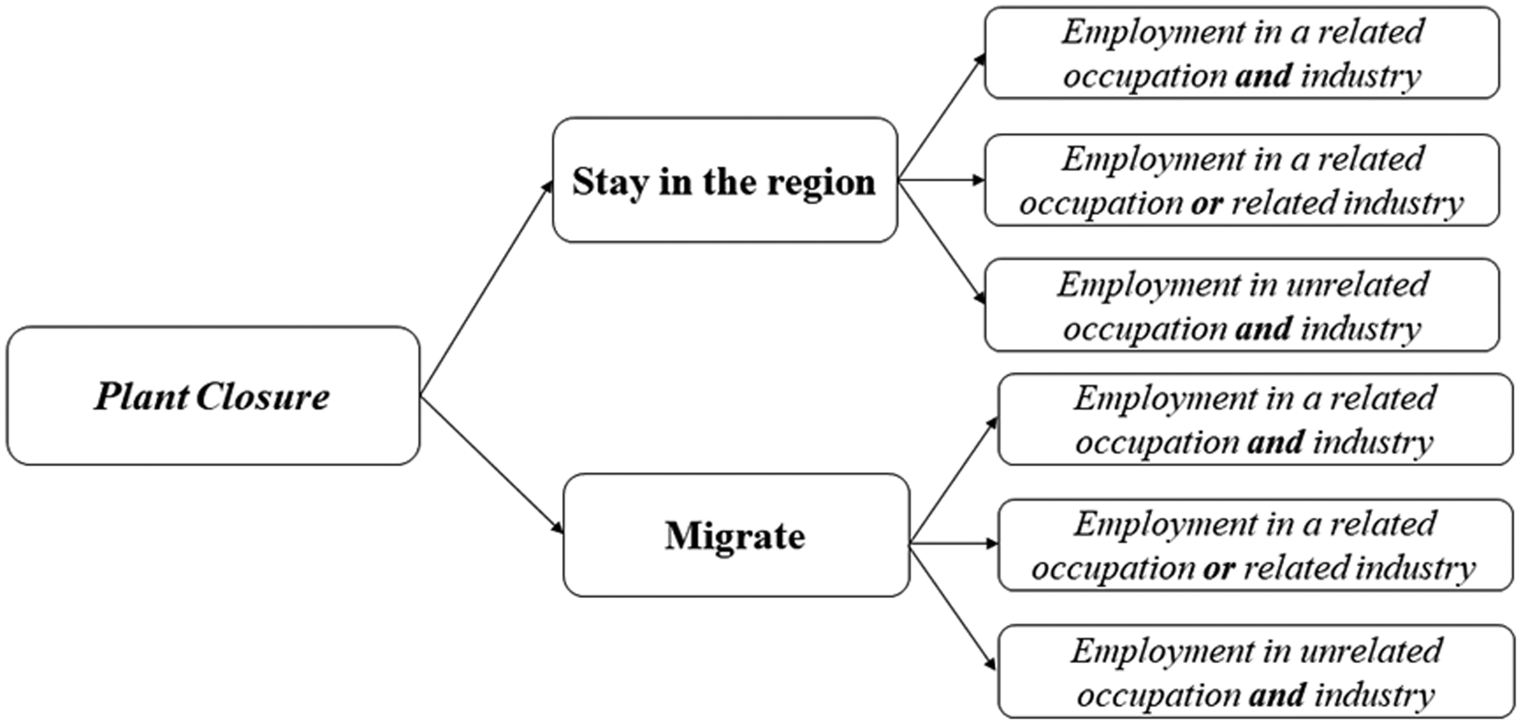
Potential labor market outcomes of displaced workers.

The indirect utility (EV_ij*) that individual i obtains by picking jth treatment (j = 0, 1, … J) is

E V_{i j}^{*} = z_{i}^{'} α_{j} + δ_{i} l_{i j} + η_{i j}

(3)

where z_i denotes the covariates with parameters α_j, and η_ij are the i.i.d distributed error terms. EV_ij* is also a function of l_ij which includes the unobserved (latent) characteristics of the individual to pick treatment j. They are assumed to be independent of η_ij. Without losing generality, let j = 0 denote the control group and

{E V}_{i 0}^{*} = 0 .

Following Abreu et al. (2015), the base category is staying in the region and getting a job in a related industry and occupation. Naturally, we cannot observe

{E V}_{i j}^{*}

, but we can observe the treatment choice of the displaced worker through a set of binary variables d_j. These are collected by a vector d _i= [d_i1, d_i2, … d_iJ], where Deb and Trivedi (2006) discuss that the probability of selecting a given strategy, conditional on latent factors, has the structure of the multinomial logit estimation

\Pr (d_{i} | z_{i}, l_{i}) = \frac{\exp (z_{i}^{'} α_{j} + l_{i j})}{1 + \sum_{k = 1}^{J} \exp (z_{i}^{'} α_{k} + l_{i k})} where j = 0, 1, 2, \dots J

(4)

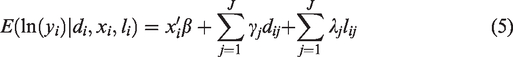
The second stage is the wage equation that explains earnings two years after displacement. All individuals are included in this step, where some of them are “treated” (migrated and/changed jobs), and some are not. The expected value of the outcome can be presented as

E (\ln (y_{i}) | d_{i}, x_{i}, l_{i}) = x_{i}^{'} β + \sum_{j = 1}^{J} γ_{j} d_{i j} + \sum_{j = 1}^{J} λ_{j} l_{i j}

(5)

where y_i is the career outcome for individual i, x_i is a set of exogenous variables associated to the parameter β, and

γ_{j}

is the vector of treatment effects relative to the control choice (stay and get related employment). Since this is a function of latent factors, the outcome is affected by the unobserved characteristics that affect selection into the treatment. Deb and Trivedi (2006) also argue that the parameters in the multinomial logit estimation need the scale of each choice equation to be normalized. The model can be estimated when the covariates are the same in the treatment and outcome variable, but it is preferable to have a few variables, i.e. exclusion restrictions, in z_i which are not included in x_i.

Variables

Selection into treatment

In the first stage, we control for the selection into the six treatment categories. The variables included have been found to matter for migration and labor outcomes (Abreu et al., 2015; Bartel, 1979; Bleakley and Lin, 2012; Eriksson et al., 2018; Nakosteen and Zimmer, 1982). However, there might be other unobserved variables, such as motivation, ability, social skills, childhood experiences, etc., which affect the outcomes after displacement as well as earnings. Since we do not have a panel setting and cannot include individual fixed effects directly, we adapt the Abowd et al. (1999) framework (henceforth AKM) where the individuals’ wage can be modelled as

\ln y_{i t} = α_{i} + ψ_{J (i t)} + x_{i t}^{'} β + ε_{i t}

(6)

y_it are the yearly earnings (ln), α_i are the individual fixed effects, and Ψ_J(I,t) denotes the establishment component of the equation. x′_it is the vector of time-variant characteristics, and where, following Card et al. (2013), the variables included are age squared, age cube, and education categories interacted with age square, age cube and time. Age square and age cube are included to ensure that the fixed effects do not capture the experience on wages (Butschek and Sauermann 2019b).⁶ We estimate equation (6), by using data of twelve years before displacement. Therefore, the model is run separately for people displaced each year. We then save α_i, which estimates the time-invariant unobservable skills of the individuals and use it as a control variable.⁷ Butschek and Sauermann (2019a) have shown that the AKM fixed effects are on average 40% correlated with the cognitive ability of the individuals.

To control for regional characteristics that might influence the decision to migrate, i.e., what we called “pushed migration,” we also include the size of the region of origin and the share of workers who are displaced in the region at the same time. Deb and Trivedi (2006) also mention that it is preferable to include a few variables in the treatment equation but not in the outcome one. We include three exclusion restrictions in the first step of the estimation, which act as instrumental variables. These variables should be correlated with the treatment, but not directly affect earnings.

Partner employed in a related industry: ⁸ We argue that if the displaced worker has a partner employed in a related industry, their social network in that kind of industry would be stronger, and therefore the probability of them ending up in an unrelated industry would be lower. This should, however, not directly affect their earnings.⁹ The correlation matrix in Table A6 also shows that the correlation between this variable and wages is only 5%.

Previous migration: This is a binary variable controlling if the worker had ever lived in another labor market before getting displaced. This is a rather common instrument used in the literature to predict migration decisions of individuals (Abreu et al., 2015; Venhorst and Cörvers, 2018); it should not impact post-displacement earnings. One could argue that the more able people are the ones who migrate and therefore migration isn’t uncorrelated to wages. While this could be true, we do not think this affects this sample, especially after looking at the correlation matrix in Table A6. The correlation between the post-displacement wage and the previous migration dummy is only 4%. The low correlation values indicate that this is not a problem.

Parents in the old region: We include a binary variable for whether at least one of the parents lives in the same labor market at the time of displacement. Given the importance of family ties (Huttunen et al., 2018), this should affect the decision of the individual to migrate, but it shouldn’t have an effect on wages. Similar arguments as above could also be made for this exclusion restriction where the correlation between wage and having parents in the region is quite low, at 2.7% (Table A6).

To test that the exclusion restrictions are correlated with the treatment, we estimate the first stage of the model with outcomes being the six migration and job relatedness variables and including the exclusion restrictions as dependent variables. Table A3 presents the multinomial estimation of the first stage of the model, with the base category being stay in the region and get a job in a related occupation and industry. This way we test the “relevance assumption” of the IV.¹⁰ We also run an OLS regression where the dependent variable is ln(y_it) and we include the three exclusion restrictions as independent variables. Results presented in Table A4 show that none of these variables are directly related to earnings. We therefore believe that our exclusion restrictions are good and valid instruments to include in the empirical estimation.

Earnings

Most variables included in the second stage of the model come from the Mincer (1974) literature. To account for regional disparities in wages, we include regional size. Since earnings also depend on the local market conditions (Jacobson et al., 1993), we include the share of total displaced workers in the region to measure how distressed a region is. Table A1 shows all the variables used in the empirical estimation.

Descriptive statistics

Table 1 presents the number of plants that employ more than 10 employees and workers (in the age ranges of 25–60).

Table 1.

Descriptive statistics on displacement.

Descriptives	2003	2004	2005	2006	2007	2008	Sample*
Number of individuals	10565	9760	9949	6646	7402	6226	26,665
Number of plants	683	644	629	501	583	470	3,030
Average size of plant	95	64	100	88	71	84	88
Reemployment rate	81%	83%	85%	87%	86%	86%
Migration rate	5%	4%	4%	5%	4%	5%	3%

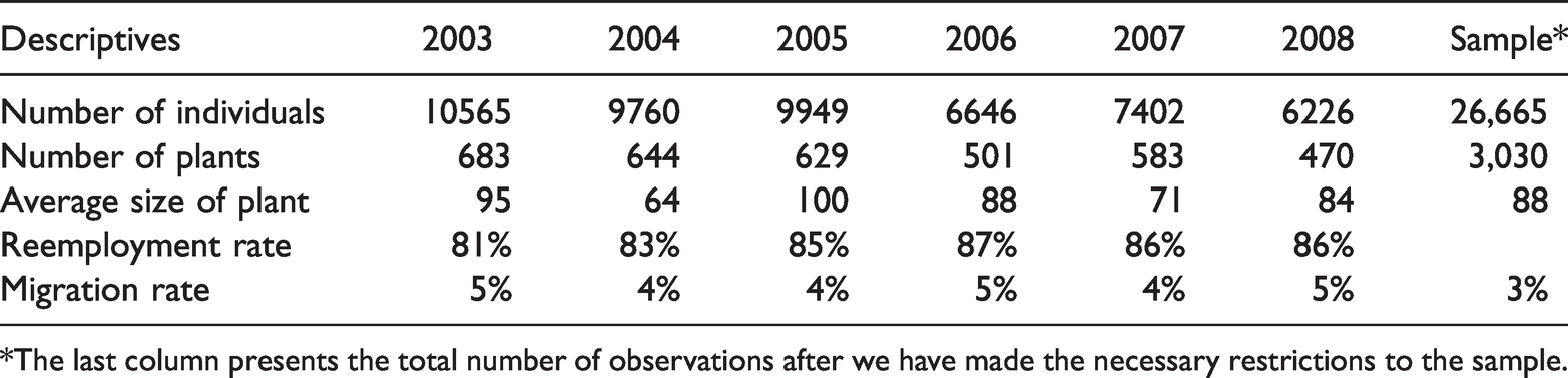
*The last column presents the total number of observations after we have made the necessary restrictions to the sample.

Restricting the sample to those who earn more than 13,600 SEK in monthly income for whom we have information on all the variables, the sample reduces to 26,665 individuals. Table 2 shows how these values vary between movers and stayers. The largest share in both groups moves to a related industry and occupation. As pointed out by Gallaway (1969), movers are slightly more likely to get employed in unrelated industries, occupations, or both. The difference is statistically significant in all cases.

Table 2.

Mobility outcomes of displaced workers.

Mobility	All (%)	Stayers (%)	Movers (%)
Related industry and occupation	70	70	66
Related industry or occupation	25	25	27
Different industry and Occupation	5	5	7

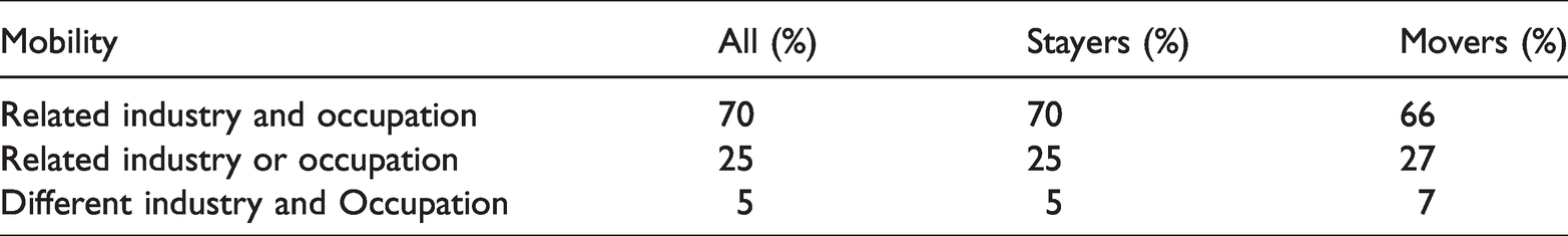
Table 3 shows the mean values for individual characteristics across the categories.¹¹ The results show the following. Displaced workers who had a higher pre-displacement average wage are the ones who get employed in a related industry and occupation, independent of migrating or not. They are also the ones who show the highest earnings post-displacement. Migrants tend to be younger. Migrants who get a job in a related industry and occupation, or only change one of them, have on average 1 more year of schooling. Regarding ability, one can also see differences across groups, even if the actual value of the variable cannot be interpreted. We see that the ones who stay in the region have on average higher unobserved ability than the ones who do not. The lowest value of ability is observed for the ones who move and get an unrelated employment. Females are also less likely to move. The ones with longer firm tenure seem to stay in the region. The income of the partner is much lower average values than the income of the displaced workers themselves. This is driven by the fact that for those who do not have partners, the value of the variable is zero. It does however show that the ones who migrate have partner with lower income, again, probably driven by non-married individuals. The partners of the ones who stay in the region and get a related job earn on average higher wages than all other categories. Displaced workers with shorter firm tenure end up more often in related industries and occupations. If the individual had migrated before, she is more likely to do so again. Having parents living in the region seems to be negatively related to migration. In addition, those who have partners employed in related occupations are less likely to migrate but are also less represented in categories on unrelated job matches.

Table 3.

Mean values for the individual characteristics for each category of displaced workers.

	Stay, related industry and occupation	Stay, related industry or occupation	Stay, unrelated industry and occupation	Move, related industry and occupation	Move, related industry or occupation	Move, unrelated industry and occupation
New wage^a	3771	3384	2859	3844	3386	2712
Previous wage^a	3406	3244	2910	3428	3175	3113
Age	43	43	43	39	39	37
School years	12	12	12	13	13	12
Ability	−0.068	−0.142	−0.222	−0.277	−0.330	−0.413
Female	0.34	0.34	0.36	0.32	0.36	0.24
Partner income	1401	1339	1207	689	867	596
Foreign-born	0.09	0.07	0.07	0.06	0.06	0.10
Firm tenure	4.67	5.25	5.72	3.64	4.43	4.37
Partner in industry	0.11	0.08	0.06	0.07	0.04	0.02
Previous migration	0.16	0.17	0.14	0.5	0.54	0.52
Parents old region	0.56	0.59	0.62	0.41	0.33	0.44

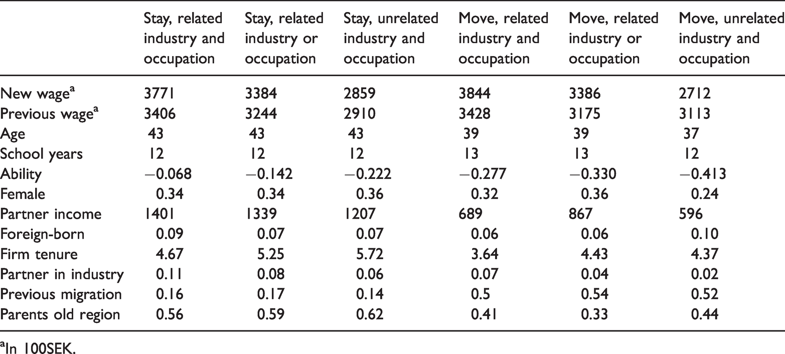
^aIn 100SEK.

Results and analysis

Table 4 reports the results of the multinomial treatment effects model using Maximum Simulated Likelihood (with 2,000 replications). Columns 1–5 are the first-stage multinomial logit model for migration, industrial, and occupational change. The base category is staying in the region and getting a job in a related industry and occupation. The results reported are relative risk ratios compared to the base category.¹² The last column is the second-stage model for earnings, two years after displacement.

Table 4.

Treatment effects model for ln(wages) two years after displacement.

	Stay, related industry or occupation	Stay, unrelated industry and occupation	Move, related industry and occupation	Move, related industry or occupation	Move, unrelated industry and occupation	ln(wage)
Previous wage	−0.332*** (0.065)	−0.808*** (0.132)	0.301* (0.159)	−0.211 (0.250)	−0.171 (0.607)	0.706*** (0.013)
Age	0.048*** (0.018)	0.060* (0.033)	−0.206*** (0.045)	−0.013 (0.073)	−0.108 (0.122)	0.040*** (0.003)
Age²	−0.001*** (0.000)	−0.001* (0.000)	0.002*** (0.001)	−0.000 (0.001)	0.001 (0.001)	−0.000*** (0.000)
School years	−0.004 (0.009)	−0.047** (0.019)	0.039 (0.024)	0.025 (0.035)	−0.104 (0.075)	0.019*** (0.002)
Ability	−0.047 (0.048)	−0.296*** (0.091)	0.159 (0.125)	0.094 (0.184)	0.092 (0.376)	0.035*** (0.009)
Female	−0.022 (0.039)	−0.018 (0.071)	0.054 (0.102)	0.179 (0.155)	−0.288 (0.329)	−0.090*** (0.007)
Partner Income	0.011** (0.005)	0.005 (0.009)	−0.133*** (0.015)	−0.088*** (0.021)	−0.090** (0.039)	0.004*** (0.001)
Foreign-born	−0.185*** (0.068)	−0.269** (0.129)	−0.372* (0.197)	−0.539* (0.302)	0.156 (0.507)	−0.084*** (0.013)
Firm tenure	0.046*** (0.005)	0.067*** (0.009)	−0.044*** (0.016)	0.045** (0.023)	0.030 (0.049)	−0.001* (0.001)
Regional Size	−0.078*** (0.013)	−0.110*** (0.024)	−0.334*** (0.034)	−0.323*** (0.053)	−0.307*** (0.106)	0.009*** (0.002)
Displaced workers	0.187*** (0.059)	0.136 (0.093)	−0.666*** (0.238)	−0.142 (0.193)	0.349 (0.278)	−0.011 (0.009)
Old firm size	−0.033** (0.016)	0.054* (0.030)	−0.056 (0.044)	0.007 (0.072)	0.074 (0.131)	0.006** (0.003)
Partner in industry	0.145*** (0.052)	0.025 (0.101)	1.208*** (0.115)	1.329*** (0.178)	1.422*** (0.354)
Previous migration	0.145*** (0.052)	0.025 (0.101)	1.208*** (0.115)	1.329*** (0.178)	1.422*** (0.354)
Parents old region	0.055 (0.040)	0.055 (0.074)	−0.463*** (0.111)	−0.853*** (0.162)	−0.427 (0.356)
Stay, Rel. Ind or Occupat.						−0.069*** (0.017)
Stay, Unrel. Ind. and Occupat.						−0.146***(0.046)
Move, Rel. Ind. and Occupat.						0.056**(0.025)
Move, Rel. Ind. or Occupat.						−0.024 (0.040)
Move, Unrel. Ind. and Occupat.						−0.197*** (0.052)
λ (Stayer, change one)						−0.017 (0.016)
λ (Stayer, change both)						0.011 (0.047)
λ (Mover, no change)						−0.061*** (0.014)
λ (Mover, change one)						−0.085*** (0.016)
λ (Mover, change both)						−0.015***(0.005)
Constant	1.442** (0.637)	3.466*** (1.243)	3.098** (1.456)	1.858 (2.412)	3.274 (5.415)	1.288*** (0.125)
Observations	26,665	26,665	26,665	26,665	26,665	26,665

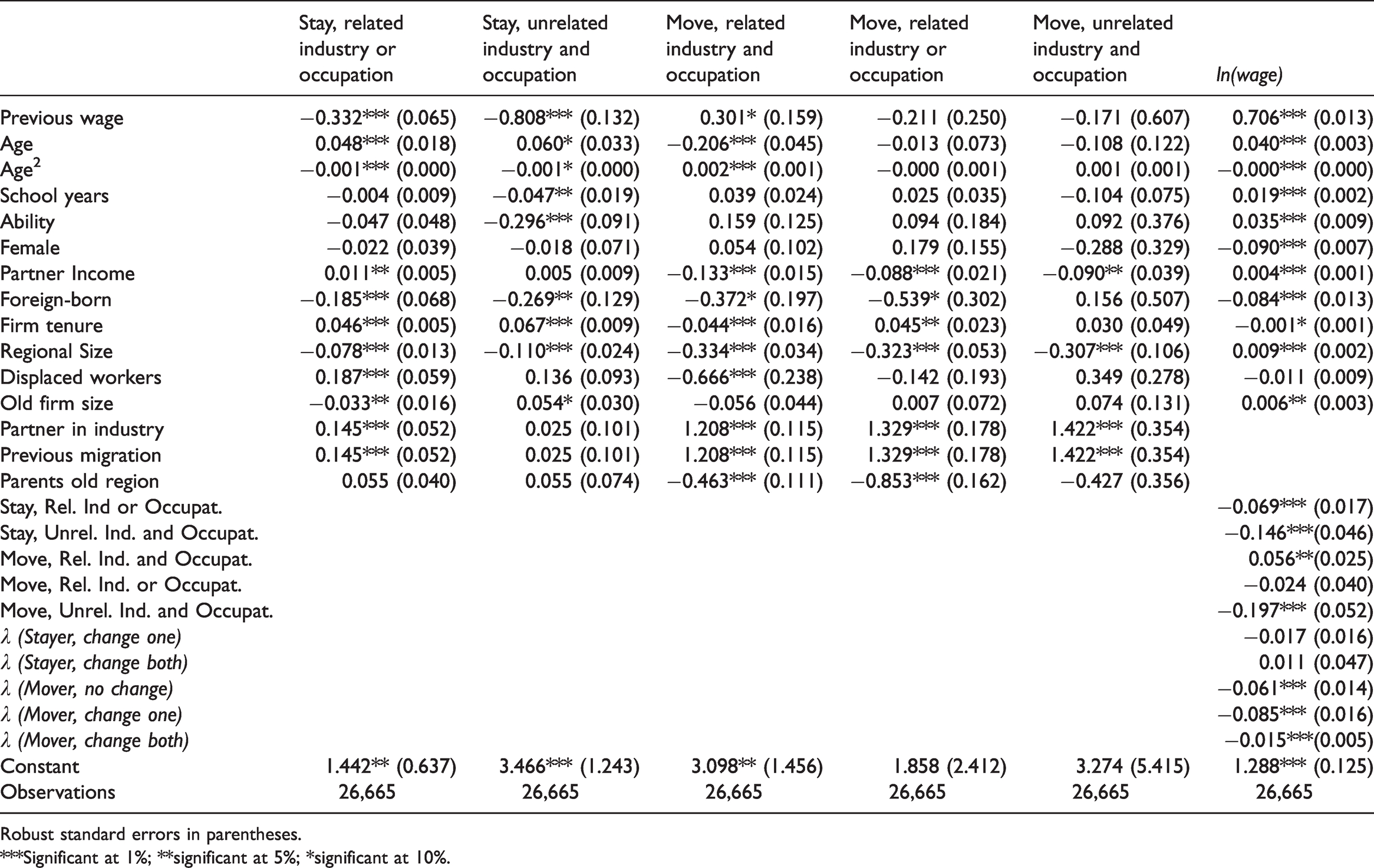
Robust standard errors in parentheses.

***Significant at 1%; **significant at 5%; *significant at 10%.

Selection into treatment (stage 1)

The first step of the estimation (columns 1–5) controls for the selection into the outcomes. Results show that those individuals who earned more before displacement are less likely to move to an unrelated job if they stay in the region. They are however more likely to migrate and get a job that matches their skills. Older individuals are less likely to migrate and get related employment compared to the base category. Rather, they are more likely to stay in the region and get an unrelated job. This is expected, given that their networks and local knowledge are more useful to them in their origin area. Those with more years of schooling and those with higher ability (AKM fixed effects) are less likely to get a job in an unrelated occupation and industry if they stay in the region. No significant gender differences are observed in this stage. The income of the partner decreases the odds of individuals migrating from the region altogether, which is expected given the fact that the cost of migration for them is higher. The foreign-born are less likely to stay in the region and get re-employed in an unrelated industry or occupation. They are also less likely to migrate in general. With longer firm tenure, the probability of switching industry, occupation, or both increases. Longer firm tenure is also associated with a lower probability of migrating and re-employment in a related job.

As for regional characteristics, living in a large region decreases the odds of moving to another region (Bleakley and Lin, 2012; Duranton and Diego, 2004). The more displaced workers in the region, the more likely they are to get re-employed in an unrelated job and the less likely they are to migrate and get a related employment. Individuals who get displaced from larger workplaces are also more likely to get employment in an unrelated industry or occupation, but no significant results are observed on the migration outcomes.

The exclusion restrictions show that workers who have migrated before are more likely to do so again, as opposed to staying in the region and getting employed in a related industry and occupation. Also, those who have parents in the region are less likely to migrate. The ones who have a partner employed in a related industry are less likely to end up in unrelated jobs, no matter if they stay in the region or not (though it is not significant in the last category).

Earnings (stage 2)

Moving on to the second stage, the estimation shows that while controlling for the endogeneity of changing location, industry, and/or occupation, migrants are better off than stayers in the base category when they get a related employment. This result is in line with Abreu et al. (2015). Movers who get a job in a related industry and occupation earn approximately 5% more than stayers. This confirms our expectation that there are positive returns to migration when the job matches the occupation- and industry- specific skills of the workers.

These positive outcomes on earnings are not observed for migrants who get employment in unrelated jobs; they are worse off than stayers who work in a related industry and occupation. Earnings are around 20% lower for those who move but find work in an unrelated industry and occupation. These results suggest that migrants are a heterogenous group, where some of them might choose to migrate because they found a job that fits them better somewhere else, while others might be pushed to do so because of a lack of better opportunities in their region of origin. The latter group is also referred to as ‘forced migrants’ (Smits, 2001; Venhorst and Cörvers, 2018). Empirically, it is difficult to identify which is the case.

As for stayers, a negative relation to the base category is observed for those with employment in a related industry or occupation, i.e., a change in only one of them. They earn on average 7% less than those who get re-employed in a related industry and occupation. Earnings are however 15% lower if they stay in the region and change both industry and occupation. The results also provide evidence of the selection on unobservables (indicated with the λ) that are statistically significant in most cases, indicating there are still characteristics we do not control for in the model.

Regarding the control variables, those who earned more before displacement also earn more two years later. The more able individuals (captured through the AKM fixed effects) are, the more they earn after displacement. So do older individuals, and those with more years of schooling. Women earn less than men after displacement, in line with Boman (2011). There is a wage premium for those whose partner is also employed. Foreign-born earn less than natives after displacement. Those who have more firm tenure seem to have lower wages, possibly due to strong firm-specific non-transferrable skills. Living in a larger region before displacement also shows a positive sign for earnings, suggesting a urban wage premium (Glaeser and Mare, 2001). There is also a wage premium for those who are displaced from larger firms.

Alternative specifications and robustness tests

To check the stability of the results, we run some alternative specifications where we only present the results for the main variables.

Monthly wage

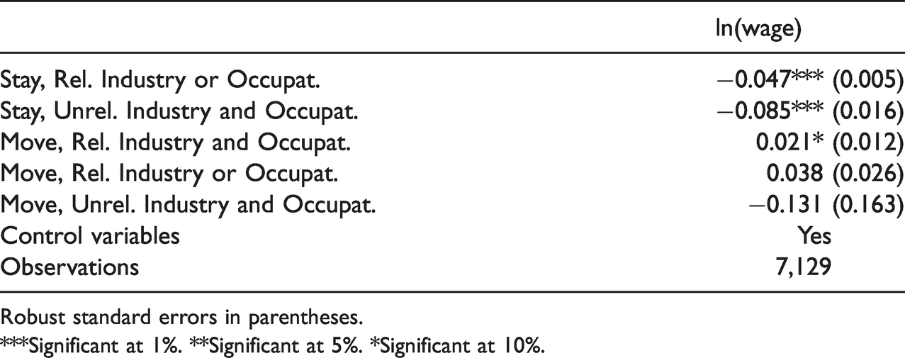
A weakness of the data is that Statistics Sweden does not gather information on hours worked, and we do therefore not know whether the individuals work full time or not. However, we have the monthly wage of a subsample of the population, which includes everyone employed in the public sector and around 50% of the workers in the private sector. This variable is not dependent on the number of hours worked, but denotes the monthly wage of the individuals, as if they would be working 100%. This way, we get closer to estimating the actual effect of migration and job change on wages. For our sample of displaced workers, the number of observations drops to 7,129 when we estimate the model with monthly wages rather than yearly ones. Table 5 indicates that migrants are better off than stayers in the base category if they get a related employment, with approximately 2% more earnings. The job match is important for earnings after displacement. However, the other two outcomes for the migrants show no statistical significance. This can be a result of the low number of observations in each of those categories. As for stayers, getting re-employed in an unrelated occupation and/or industry means lower earnings than the ones in the base category.

Table 5.

Treatment effects model for ln(monthly wages) two years after displacement.

	ln(wage)
Stay, Rel. Industry or Occupat.	−0.047*** (0.005)
Stay, Unrel. Industry and Occupat.	−0.085*** (0.016)
Move, Rel. Industry and Occupat.	0.021* (0.012)
Move, Rel. Industry or Occupat.	0.038 (0.026)
Move, Unrel. Industry and Occupat.	−0.131 (0.163)
Control variables	Yes
Observations	7,129

Robust standard errors in parentheses.

***Significant at 1%. **Significant at 5%. *Significant at 10%.

Other robustness checks

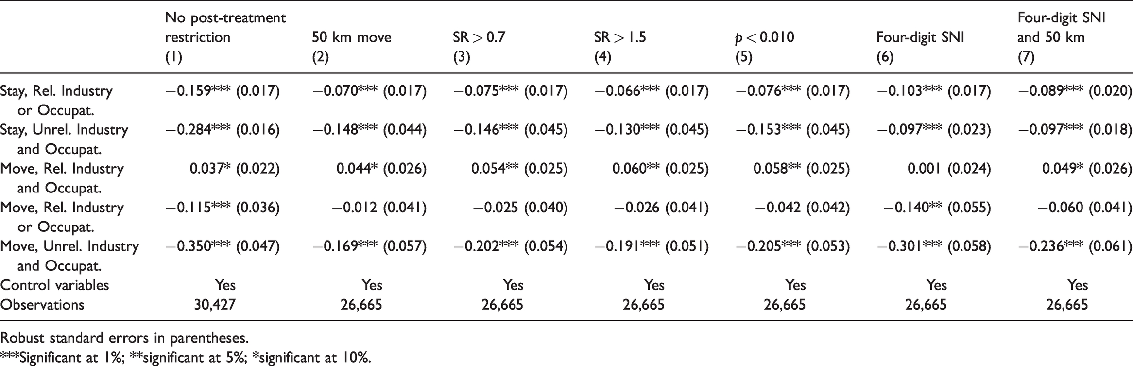
In the baseline regression, we condition the treatment estimations on individuals who do not receive unemployment benefits in t + 2 to be able to compare the wages of workers who have worked throughout the years. This way we can make meaningful comparisons, given that we have no information on days or hours worked in a year. However, by doing so, we condition our sample on post-treatment outcomes, which can give biased results (Montgomery et al., 2018). We therefore run the estimation without any restrictions in t + 2. Results are shown in the first column of Table 6 and are robust to the main specification, even though the magnitudes of wages are different. This is not surprising given that individuals who migrate are less likely to find a job (see the discussion in footnote 12), and they might even wait longer to get employment on average, even if we do not know this with certainty. We therefore do not interpret the coefficients, but we can at least to some extent ensure that the post-treatment restriction we make on the data does not affect the main findings.

Table 6.

Different robustness checks for the treatment effects model for returns to migration and job relatedness. ln(wage t2) is the dependent variable in all the estimations.

	No post-treatment restriction	50 km move	SR > 0.7	SR > 1.5	p < 0.010	Four-digit SNI	Four-digit SNI and 50 km
	(1)	(2)	(3)	(4)	(5)	(6)	(7)
Stay, Rel. Industry or Occupat.	−0.159*** (0.017)	−0.070*** (0.017)	−0.075*** (0.017)	−0.066*** (0.017)	−0.076*** (0.017)	−0.103*** (0.017)	−0.089*** (0.020)
Stay, Unrel. Industry and Occupat.	−0.284*** (0.016)	−0.148*** (0.044)	−0.146*** (0.045)	−0.130*** (0.045)	−0.153*** (0.045)	−0.097*** (0.023)	−0.097*** (0.018)
Move, Rel. Industry and Occupat.	0.037* (0.022)	0.044* (0.026)	0.054** (0.025)	0.060** (0.025)	0.058** (0.025)	0.001 (0.024)	0.049* (0.026)
Move, Rel. Industry or Occupat.	−0.115*** (0.036)	−0.012 (0.041)	−0.025 (0.040)	−0.026 (0.041)	−0.042 (0.042)	−0.140** (0.055)	−0.060 (0.041)
Move, Unrel. Industry and Occupat.	−0.350*** (0.047)	−0.169*** (0.057)	−0.202*** (0.054)	−0.191*** (0.051)	−0.205*** (0.053)	−0.301*** (0.058)	−0.236*** (0.061)
Control variables	Yes	Yes	Yes	Yes	Yes	Yes	Yes
Observations	30,427	26,665	26,665	26,665	26,665	26,665	26,665

Robust standard errors in parentheses.

***Significant at 1%; **significant at 5%; *significant at 10%.

We defined migration as moves across labor market borders. However, it can be the case that individuals live close to the labor market borders and the move does not necessarily imply migration. Given that we have geo-coded data on where individuals live, another robustness check we did is to define migrants as those who have moved at least 50 km after displacement. The results are shown in the second column of Table 6: they are in line with the baseline estimation. Movers with a related employment earn more than stayers in the same category and those who get unrelated jobs are still worse off.

The third set of robustness tests deals with how we define relatedness. We defined skill-related industries and occupations if the SR measure (equation (1)) is larger than one and the p-value (equation (2)) is lower than 5%. To ensure that these are not too restrictive, we adjust the definition by defining skill-relatedness as SR> 0.7 and SR > 1.5 (columns 3 and 4 in Table 6). Even here the results are in line with what is presented in the baseline estimation. In column 5, skill relatedness is defined as above 1 with a p-value less than 10%. A similar pattern is observed in this case as well, where migrants with a related employment are better off than the stayers. Now, migrants who get employed in a related industry or occupation (only one of the dimensions is unrelated) show that they earn less than stayers who get a related job.

In column 6, results are presented with skill-relatedness measured with 4-digit SNI codes. While the results look like the baseline ones, the wage of movers who get employed in a related job is now not statistically different than stayers. For that reason, we re-estimated the same model with 4-digit SNI codes when migration is defined as moves greater than 50 km, instead of moves across labor markets. These results are presented in column 7. Now, migrants who get a related employment are again better off than stayers in the base category, with about 5% higher earnings. Therefore, we argue that the results after all the robustness tests are very similar to the baseline estimations and our main conclusions still hold.

Concluding remarks

This paper expands the discussion on returns to migration of displaced workers by accounting for the type of jobs they get and how this matches their skills. It builds on studies that have looked at mechanisms why displaced workers experience earnings losses (Carrington, 1993; Kambourov and Manovskii, 2009; Neal, 1995) and combines it with the skill-relatedness literature (Neffke and Henning, 2013) that has shown that labor mobility across related industries and occupations may have positive economic outcomes (Boschma et al., 2008; Cappelli et al., 2019; Jara-Figueroa et al., 2018; Timmermans and Boschma, 2014).

We find that displaced workers that migrate are, on average, slightly more likely to get employed in unrelated industries and occupations. However, migrants who get employed in an occupation and industry related to their pre-displacement one have higher wages than those who stay in the region and get a related employment, making them the group that experiences the highest earnings after migration. In contrast, migrants who get a job in an unrelated occupation and industry experience lower earnings than the base category. This group actually shows the lowest earnings after displacement. Stayers who do not find a suitable employment for their occupation and industry-specific skills exhibit low earnings, but not as low as migrants in that category.

These results have policy relevance, given that displacement is now and then associated with high costs for individuals as well as for society. Our findings suggest that migration is not necessarily the key mechanism that matters for future earnings, but job match is. Those who migrate and get an unrelated employment experience the highest earning losses, compared to the base category of stayers with a related job. This finding implies a need for policy intervention programs that facilitate the job match between workers and firms by incorporating a broader view of job matching that also includes skill-related activities. This suggests that policy focused on job-matching should not only look at educational levels of displaced workers, but also account for the type of industry- and job-specific skills displaced workers have. It implies that any policy should be tailor-made and targeted to specific groups. In regions with many skill-related industries around, the need for strong policy intervention is low, as displaced workers can find job opportunities in which their skills are still relevant. Our findings suggest that policy is especially relevant for displaced workers that move to another region, because there is a higher likelihood of poor job-matching, with individual and social welfare losses as a result. This implies that policy should be very keen on this group of migrants and focus on their smooth integration in the regional labor market through information provision and active re-integration programs.

Another group of displaced workers that requires special policy attention consists of displaced workers that got displaced from jobs that face low demand for their skills in general (for example, due to automation of specific job-skills, see Autor et al., 2003), and those that live in regions with no or few skill-related industries. In these circumstances, a strong policy of re-education rather than job-matching efforts is needed to ensure that displaced workers get re-integrated into the labor market so as to get access to better jobs. Another type of policy is to ensure that there is a substantial local presence of skill-related industries in a region in order to ensure that displaced workers will be absorbed by the local labor market. This can be stimulated by an active industrial and diversification policy that encourages the development of new industries or jobs that are skill-related to local activities in the region (Balland et al., 2019). This also enhances the resilience of regions to shocks, as studies have shown that a local supply of skill-related industries can act as an effective shock-absorber in regions (Boschma, 2015; Diodato and Weterings, 2014).

This study has its limitations. First, the lack of hourly wage data for the full displaced population could be improved in future studies for greater accuracy. Second, it would be interesting to study this in a panel setting where individuals are tracked over a longer period to see the wage development. Another empirical challenge we face is that we only observe those workers who get re-employed. What we cannot measure is whether the alternative to an unrelated employment is being without a job. People may be pushed into migration and unrelated employment. This is difficult to estimate since we do not observe job offers. One way to extend it is by focusing on the regional characteristics and how the regions shape the labor outcomes for stayers as well as for migrants, and whether that is reflected in their wages.

Footnotes

Declaration of conflicting interests

The author(s) declared no potential conflicts of interest with respect to the research, authorship, and/or publication of this article.

Funding

The author(s) received no financial support for the research, authorship, and/or publication of this article.

ORCID iD

Orsa Kekezi

Notes

References

Abowd

Kramarz

Margolis

(1999) High wage workers and high wage firms. Econometrica 67(2): 251–333.

Abreu

Faggian

McCann

(2015) Migration and inter-industry mobility of UK graduates. Journal of Economic Geography 15(2): 353–385.

Ahlin

Andersson

Thulin

(2014) Market thickness and the early labour market career of university graduates: An urban advantage? Spatial Economic Analysis 9(4): 396–419.

Autor DH, Frank L and Murnane RJ (2003) The Skill Content of Recent Technological Change: An Empirical Exploration. The Quarterly Journal of Economics 118(4): 1279–1333.

Axelsson

Westerlund

(1998) A panel study of migration, self-selection and household real income. Journal of Population Economics 11(1): 113–126.

Balland P-A, Boschma R, Crespo J and Rigby DL (2019) Smart specialization policy in the European Union: relatedness, knowledge complexity and regional diversification. Regional Studies 53(9): 1252–1268.

Bartel

(1979) The migration decision: What role does job mobility play? The American Economic Review 69(5): 775–786.

Basile

Lim

(2017) Nonlinearities in interregional migration behavior: Evidence from the United States. International Regional Science Review 40(6): 563–589.

Becker

(1962) Investment in human capital: A theoretical analysis. Journal of Political Economy 70(5): 9–49.

10.

Bleakley

Lin

(2012) Thick-market effects and churning in the labor market: Evidence from US cities. Journal of Urban Economics 72(2–3): 87–103.

11.

Böheim

Taylor

(2007) From the dark end of the street to the bright side of the road? The wage returns to migration in Britain. Labour Economics 14(1): 99–117.

12.

Boman

(2011) Does migration pay? Earnings effects of geographic mobility following job displacement. Journal of Population Economics 24(4): 1369–1384.

13.

Borjas

(1987) Self-selection and the earnings of immigrants. Americal Economic Review 77(4): 531–553.

14.

Boschma R (2015) Towards an Evolutionary Perspective on Regional Resilience. Regional Studies 49(5): 733–751.

15.

Boschma

Eriksson

Lindgren

(2014) Labour market externalities and regional growth in Sweden: The importance of labour mobility between skill-related industries. Regional Studies 48(10): 1669–1690.

16.

Boschma

Eriksson

Lindgren

(2008) How does labour mobility affect the performance of plants? The importance of relatedness and geographical proximity. Journal of Economic Geography 9(2): 169–190.

17.

Butschek

Sauermann

(2019a) Do estimated individual fixed effects capture worker ability? Stockholm University [Unpublished work].

18.

Butschek

Sauermann

(2019b) The effect of employment protection on firms’ worker selection. IZA Discussion Paper No. 12305, Available at SSRN: https://ssrn.com/abstract=3390295

19.

Cappelli

Boschma

Weterings

(2019) Labour mobility, skill-relatedness and new plant survival across different development stages of an industry. Environment and Planning A: Economy and Space 51(4): 869–890.

20.

Card

Heining

Kline

(2013) Workplace heterogeneity and the rise of west German wage inequality. The Quarterly Journal of Economics 128(3): 967–1015.

21.

Carrington

(1993) Wage losses for displaced workers: Is it really the firm that matters? The Journal of Human Resources 28(3): 435–462.

22.

Couch

Placzek

(2010) Earnings losses of displaced workers revisited. The American Economic Review 100(1): 572–589.

23.

Cox

(1971) The effect of geographic and industry mobility on income: A further comment. The Journal of Human Resources 6(4): 525–527.

24.

Deb

Trivedi

P K

(2006) Specification and simulated likelihood estimation of a non‐normal treatment‐outcome model with selection: Application to health care utilization. The Econometrics Journal 9(2): 307–331.

25.

Di Cintio

Grassi

(2017) International mobility and wages: An analysis of Italian Ph.D. graduates. The Annals of Regional Science 59(3): 759–791.

26.

Diodato

Weterings

ABR

(2014) The resilience of regional labour markets to economic shocks: Exploring the role of interactions among firms and workers. Journal of Economic Geography 15(4): 723–742.

27.

Dostie

Léger

(2009) Self-selection in migration and returns to unobservables. Journal of Population Economics 22(4): 1005–1024.

28.

Duranton

Diego

(2004) Micro-foundations of urban agglomeration economies. In: Vernon Henderson

Jacques-François

(eds) Handbook of Regional and Urban Economics. Amsterdam: Elsevier, 2063–2117.

29.

Eliason

Storrie

(2006) Lasting or latent scars? Swedish evidence on the long‐term effects of job displacement. Journal of Labor Economics 24(4): 831–856.

30.

Eriksson

Hane-Weijman

Henning

(2018) Sectoral and geographical mobility of workers after large establishment cutbacks or closures. Environment and Planning A: Economy and Space 50(5): 1071–1091.

31.

Fackler

Rippe

(2017) Losing work, moving away? Regional mobility after job loss. LABOUR 31(4): 457–479.

32.

Gallaway

(1969) The effect of geographic labor mobility on income: A brief comment. The Journal of Human Resources 4(1): 103–109.

33.

Gathmann

Helm

Schönberg

(2020) Spillover effects of mass layoffs. Journal of the European Economic Association 18(1): 427–468.

34.

Gathmann

Schönberg

(2010) How general is human capital? A task‐based approach. Journal of Labor Economics 28(1): 1–49.

35.

Glaeser

Mare

(2001) Cities and skills. Journal of Labor Economics 19(2): 316–342.

36.

Grant

Vanderkamp

(1980) The effects of migration on income: A micro study with Canadian data 1965-71. The Canadian Journal of Economics. Revue Canadienne D'economique 13(3): 381–406.

37.

Greenwood

(1975) Research on internal migration in the United States: A survey. Journal of Economic Literature 13(2): 397–433.

38.

Greenwood

(1985) Human migration: Theory, models, and empirical studies. Journal of Regional Science 25(4): 521–544.

39.

Herzog

Schlottmann

Boehm

(1993) Migration as spatial job–search: A survey of empirical findings. Regional Studies 27(4): 327–340.

40.

Huttunen

Møen

Salvanes

(2018) Job loss and regional mobility. Journal of Labor Economics 36(2): 479–509.

41.

Isserman

Carol

Shelby

, et al. (1987) Regional labor market analysis. In: Handbook of Regional and Urban Economics. Amsterdam: Elsevier, pp. 543–580.

42.

Jacobson

Robert

Daniel

(1993) Earnings losses of displaced workers. The American Economic Review 83(4): 685–709.

43.

Jara-Figueroa

Jun

Glaeser

, et al. (2018) The role of industry-specific, occupation-specific, and location-specific knowledge in the growth and survival of new firms. Proceedings of the National Academy of Sciences of the United States of America 115(50): 12646–12653.

44.

Kambourov

Manovskii

(2009) Occupational specificity of human capital. International Economic Review 50(1): 63–115.

45.

Korpi

Martin

, William

A V Clark

Malmberg

(2010) The urban hierarchy and domestic migration: The interaction of internal migration, disposable income and the cost of living, Journal of Economic Geography Sweden 1993–2002 11(6): 1051–1077.

46.

Krieg

(1997) Occupational change, employer change, internal migration, and earnings. Regional Science and Urban Economics 27(1): 1–15.

47.

LO-tidningen (2006) Tjänstemannafack har sämsta lägstalönerna. LO-tidningen. Accessed 17 February 2020.

48.

Maddala

(1983) Limited-Dependent and Qualitative Variables in Econometrics. New York: Cambridge University Press.

49.

Mincer

(1974) Schooling, Experience, and Earnings. New York: National Bureau of Economics Research.

50.

Montgomery

Nyhan

Torres

(2018) How conditioning on posttreatment variables can ruin your experiment and what to do about it. American Journal of Political Science 62(3): 760–775.

51.

Nakosteen

Westerlund

(2004) The effects of regional migration on gross income of labour in Sweden. Papers in Regional Science 83(3): 581–595.

52.

Nakosteen

Zimmer

(1982) The effects on earnings of interregional and interindustry migration. Journal of Regional Science 22(3): 325–341.

53.

Neal

(1995) Industry-specific human capital: Evidence from displaced workers. Journal of Labor Economics 13(4): 653–677.

54.

Nedelkoska

Frank

Wiederhold

(2015) Skill mismatch and the costs of job displacement. Annual Meeting of the American Economic Association: Boston, MA.

55.

Neffke

Henning

(2013) Skill relatedness and firm diversification. Strategic Management Journal 34(3): 297–316.

56.

Neffke

Otto

Hidalgo

(2018) The mobility of displaced workers: How the local industry mix affects job search. Journal of Urban Economics 108: 124–140.

57.

Ong

Mar

(1992) Post-layoff earnings among semiconductor workers. ILR Review 45(2): 366–379.

58.

Pekkala

Tervo

(2002) Unemployment and migration: Does moving help? The Scandinavian Journal of Economics 104(4): 621–639.

59.

Poletaev

Robinson

(2008) Human capital specificity: Evidence from the dictionary of occupational titles and displaced worker surveys. Journal of Labor Economics 26(3): 387–420.

60.

Ritchey

(1976) Explanations of migration. Annual Review of Sociology 2(1): 363–404.

61.

Robinson

(2018) Occupational mobility, occupation distance, and specific human Capital. Journal of Human Resources 53(2): 513–551.

62.

Roy

(1951) Some thoughts on the distribution of earnings. Oxford Economic Papers 3(2): 135–146.

63.

Shaw

(1991) The influence of human capital investment on migration and industry change. Journal of Regional Science 31(4): 397–416.

64.

Sjaastad

(1962) The costs and returns of human migration. Journal of Political Economy 70(5, Part 2): 80–93.

65.

Smits

(2001) Career migration, self-selection and the earnings of married men and women in The Netherlands, 1981-93. Urban Studies 38(3): 541–562.

66.

Sullivan

(2010) Empirical evidence on occupation and industry specific human capital. Labour Economics 17(3): 567–580.

67.

Thurow

(1975) Generating inequality. New York: Basic books.

68.

Timmermans

Boschma

(2014) The effect of intra- and inter-regional labour mobility on plant performance in Denmark: The significance of related labour inflows. Journal of Economic Geography 14(2): 289–311.

69.

Venhorst

Cörvers

(2018) Entry into working life: Internal migration and the job match quality of higher-educated graduates. Journal of Regional Science 58(1): 116–140.

70.

Wilson

(1985) Migration and occupational mobility: A research note. International Migration Review 19(2): 278–292.

71.

Yankow

(2003) Migration, job change, and wage growth: A new perspective on the pecuniary return to geographic mobility. Journal of Regional Science 43(3): 483–516.

Returns to migration after job loss—The importance of job match

Abstract

Keywords

Introduction

Returns to migration and job (mis)match

Data, method, and variables

Defining migration and job (mis)match

Model specification

Variables

Selection into treatment

Earnings

Descriptive statistics

Results and analysis

Selection into treatment (stage 1)

Earnings (stage 2)

Alternative specifications and robustness tests

Monthly wage

Other robustness checks

Concluding remarks

Footnotes

Declaration of conflicting interests

Funding

ORCID iD

Notes

References