Sage Journals: Discover world-class research

Abstract

A harmonograph is a mechanical device driven by one or more pendulums that produces aesthetically pleasing geometric designs. For a lateral harmonograph the pictures produced are 2D projections of 2n phase space where n is the number of pendulums. The pendulums can be simple pendulums or conical pendulums. In this paper mathematical models for a 2-pendulum and 3-pendulum lateral harmonograph are derived. A small subset of parameter space is explored by analysing a number of simulations. The simulations demonstrate what the two models are capable of. A harmonograph is an excellent device to model and use as an educational tool as it can be used to engage mechanical engineering students with dynamics. It shows engineering students that a pendulum or multiple pendulums are a dynamic system that should be taken seriously and is far more interesting than an undergraduate student might superficially consider it to be.

Keywords

Dynamic system oscillating system lissajous curve lateral harmonograph

Introduction

Harmonographs are mechanical devices that use pendulums to control the motion of a pen on a sheet of paper placed on a platform. The platform can also oscillate from side to side or rotate. The harmonograph draws geometric patterns on the paper. The geometric patterns are 2-dimensional projections of 2n dimensional phase space where n is the number of pendulums. The pattern produced depends on the natural frequencies of the pendulums and the initial conditions for the pendulum motion. The pattern produced can be a geometric design that is aesthetically pleasing, or it might resemble a space filling curve that is not of much interest. Harmonographs have a role in engaging students of mechanical engineering in the mechanical engineering science, dynamics.

There is a long-standing issue with engineering students and the application of mathematics to mechanical engineering science. It is well known that over the last few decades the mathematical ability of engineering and science students has deteriorated. This is a particular problem in engineering mechanics.^1–3 The problem with poor mathematical skills of engineering students was recently reviewed.⁴ The reasons for this are complex and a detailed analysis of the issues is beyond the present article. One issue is an inability to make connections between the mathematics taught and the mechanical systems of interest. There have been many attempts to support students and find a solution to this problem.^5,6 One approach is the use of virtual learning environments (VLEs)⁷ or graphical user interfaces (GUIs).⁸ GUIs are computational tools that make it possible to explore parameter space for a dynamical system without a deep understanding of the mathematical basis of the system or the computational implementation of the model.

When trying to motivate students and identify links between mathematics and dynamical systems, one final possibility is to take a dynamic system that students are familiar with but maybe are not aware of some of the unusual or counter intuitive behaviour the system can exhibit. The simple pendulum is such a system. It is a device that is often considered early in the dynamic analysis syllabus. Most students are aware of the property that for small angular displacements the period is independent of the amplitude such that they can be used to keep time.⁹ A dynamics course including the analysis of a pendulum will often discuss resonance, the behaviour of a pendulum when forced at its natural frequency. Once the more straightforward properties of simple pendulums are discussed they are often put to one side and the lecturer moves on. There is a host of counterintuitive dynamic behaviour a simple pendulum exhibits that would greatly enhance the students experience and promote student enthusiasm for the subject. Examples of counter-intuitive pendulum dynamics are the unstable vertical-up orientation of a pendulum is stabilised if it is vertically forced at high frequency,⁸ and if a simple pendulum is forced then for certain ranges of parameter values the deterministic model demonstrates bifurcations that lead to chaotic trajectories.¹⁰

As well as the papers cited above, there are many papers in the mechanical engineering education literature where the focus is on different ways of enhancing the student experience using a simple pendulum. Big-Alabo¹¹ used the continuous piecewise linearisation method to accurately calculate the period of a simple pendulum for moderate and large amplitude oscillations. Another suggestion for enhancing the student experience using a simple pendulum is Stein et al.¹² where a desk top experiment is developed that demonstrates the functional relationship between the period of oscillation and the initial amplitude of the pendulum and demonstrates the period of oscillation dependency on the length of the pendulum.

Harmonographs are a mechanical device that demonstrates in a visual way that a relatively simple devise, a pendulum or multiple pendulums can produce both surprizing and interesting simulations. This will be discussed further below. The author has used this model to engage with mechanical engineering undergraduates taking introductory courses and intermediate courses in dynamics. This is of benefit as dynamics is a highly mathematical area that some of the weaker students regard as something to be endured rather than enjoyed.

This paper is the latest in a series of papers in the literature with the theme of taking a mechanical system that students are familiar with and presenting the mathematical basis and simulation of the respective models.^13–15 The students are engaged by the counter-intuitive behaviour or can view the more advanced models as beacons of what is possible in dynamics.

Turning to the historical development of harmonographs. The first ever harmonograph is a ‘Y’ suspended pendulum, invented by James Dean in 1815 and analysed by Nathaniel Bowditch.¹⁶ Hugh Blackburn reinvented the ‘Y’ suspended pendulum in 1844 with the device taking his name, the Blackburn pendulum.¹⁷ The Blackburn pendulum has the property that it can oscillate in two perpendicular directions with different natural frequencies. Depending on the initial conditions the pendulum bob of a Blackburn pendulum follows a trajectory similar to a Lissajous curve.¹⁸ Lissajous curves have the form.

x_{H} = A_{x} \sin (ω_{x} t + p_{x})

y_{H} = A_{y} \sin (ω_{y} t)

(1)

where the curve generated depends on the amplitudes, A_x and A_y, the natural frequencies, ω_x and ω_y and the phase p_x. Lissajous curves have applications in generating search patterns,¹⁸ the interpretation of the combination of different frequencies to produce music¹⁹ and the solution of oscillating systems consisting of two masses coupled by springs satisfying Hooke's law.²⁰

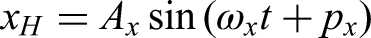
It is more usual for harmonographs to have two, three or four pendulums. Up to two pendulums controlling the motion of the pen and up to two pendulums controlling the platform the sheet of paper is on. The more pendulums used, the potentially more intricate the pattern that can be produced. The pendulums can be lateral pendulums, oscillating in a plane or rotary pendulums. For the rotary pendulums the pivot is a gimbal mechanism that allows orbital motion much the same as a conical pendulum.^13,21

The harmonograph is a mechanical device that exhibits the rich dynamic behaviour of pendulums. At present there is little in the literature on the mathematical analysis of such systems. A simple empirical model for the trajectory of the pen in a harmonograph is possible by introducing energy dissipation due to the resistive force of the pen traversing the paper and including the phase p_y.

x_{H} = A_{x} \sin (ω_{x} t + p_{x}) e^{- d_{x} t}

y_{H} = A_{y} \sin (ω_{y} t + p_{y}) e^{- d_{y} t}

(2)

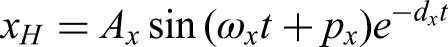
This parameterisation for the geometric pattern generated by a harmonograph is convenient for programming the generation of curves of this form, but it is not the complete solution. There is no link to the dynamic analysis of a harmonograph and the curves are “harmonograph” like. It is not possible to take a picture generated by a harmonograph and parameterise it using (2). The best that can be done is a curve fitting exercise such that the trajectory for early time is reproduced.

There are papers on the history of harmonographs and advice on how to fabricate a harmonograph.^22,23 There is little on the mathematical modelling of harmonographs in the literature. The small angle approximation to a damped simple pendulum is used to model the dynamics of two pendulums oscillating at right angles to one another.²⁴ The pendulum model has an analytical solution of the form (2). A 2-pendulum harmonograph is simulated using ProEngineer software to prescribe the kinematics. The harmonograph model produces geometric patterns similar to Lissajous curves but the simulations are initiated by prescribing the initial conditions of the pendulums.²⁴ This is a weakness as in a real harmonograph the initial conditions for the pendulum motion are prescribed indirectly by a user initially driving the motion of the pen.

There is nothing in the engineering education literature of relevance to the mathematical modelling of harmonographs. This deficiency in the literature is important as a model of a harmonograph strengthens the linkage between the mechanical device, the important physical phenomena, mathematical basis and the geometric designs generated. This paper addresses this deficiency by investigating a 2-pendulum lateral harmonograph model that is then extended to a 3-pendulum lateral harmonograph. How the mathematical models of harmonographs could be used to enhance the engineering students learning experience is also considered.

2-Pendulum harmonograph model

The type of harmonograph considered is a fixed platform 2-pendulum lateral harmonograph. The two pendulums oscillate at right angles to each other and the pen is connected to the two pendulums by light rods, see Figure 1.

Figure 1.

Sketch of a 2-pendulum lateral harmonograph.

Simple pendulum model

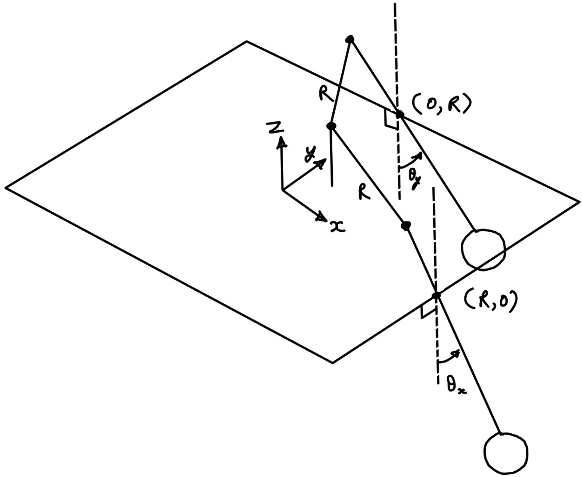
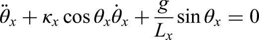
A plan view of the harmonograph is given in Figure 2. Considering the dynamics of the pendulum with a pivot located at (R, 0). The free body diagram and mass acceleration diagram for the simple pendulum are given in Figure 3. Taking a moment at the pivot and applying Newton's 2nd law gives,

I {\ddot{θ}}_{x} = - m g L_{x} \sin θ_{x} - T_{f r i c} - F_{p e n, x} L_{p e} \cos θ_{x}

(3)

where I is the mass moment of inertia of the pendulum, T_fric is the frictional loss associated with the friction at the pivot and, F_{pen, x} is the component of the resistive force acting in the plane of the pendulums motion. The frictional torque is small compared to the induced torque produced by the pens resistance to motion, meaning T_fric can be neglected. The pendulum bob can be approximated as a point mass meaning the mass moment of inertia is,

I = m L_{x}^{2}

(4)

Figure 2.

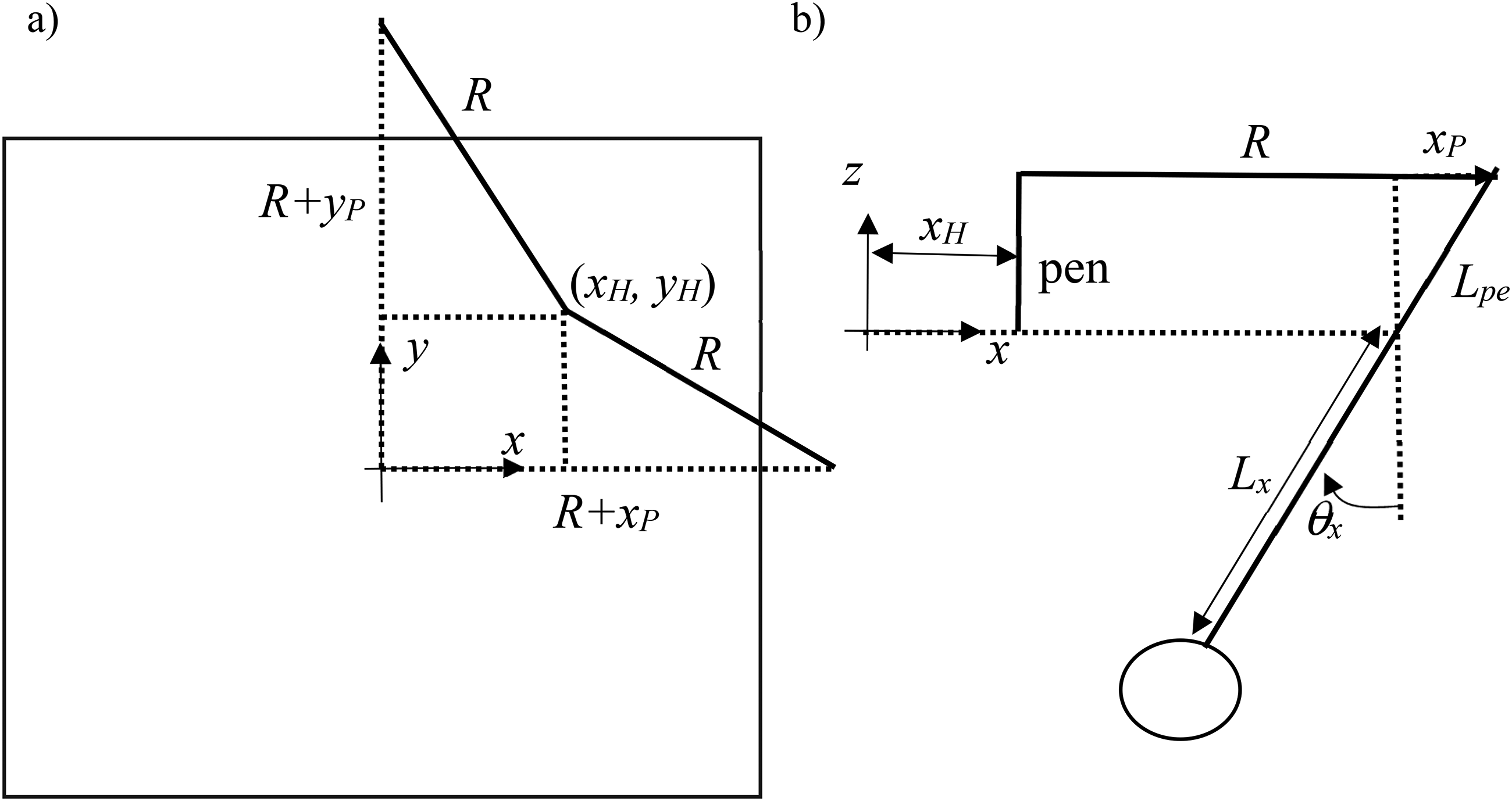
(a) Plan view and (b) side view of a lateral harmonograph.

Figure 3.

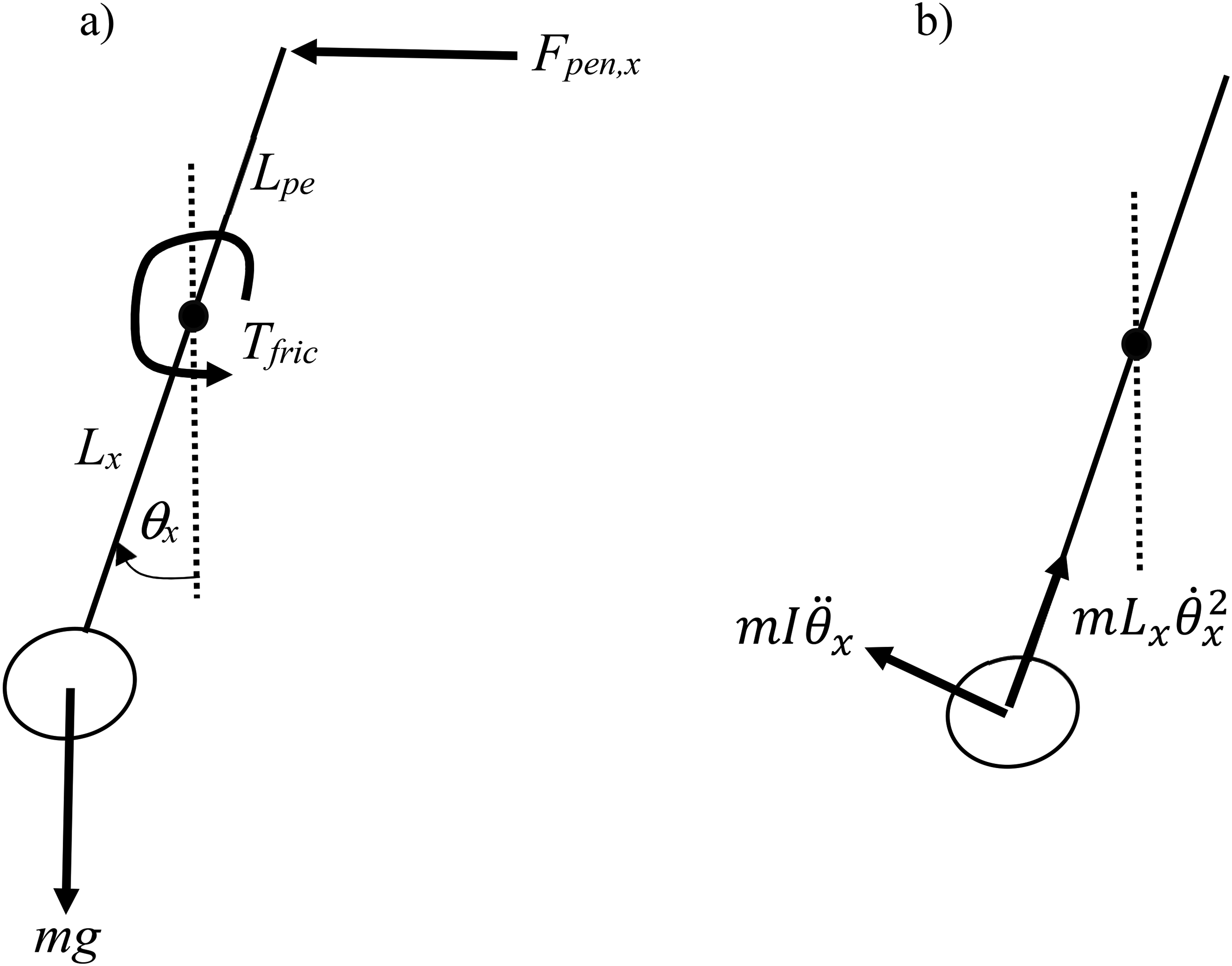
(a) Free body diagram and (b) mass acceleration diagram for a pendulum.

The final approximation introduced is the resistive force of the pen on the pendulums motion is modelled as,

F_{p e n, x} = K_{p e n} {\dot{θ}}_{x}

(5)

where K_pen is a constant. The model for the resistive force for the pen has been used previously.²⁴ All of these assumptions and approximations give the initial value problem,

{\ddot{θ}}_{x} + κ_{x} \cos θ_{x} {\dot{θ}}_{x} + \frac{g}{L_{x}} \sin θ_{x} = 0

κ $_{x} = (\frac{K_{p e n}}{m}) (\frac{L_{p e}}{L_{x}^{2}})

θ_{x} (0) = θ_{x, 0}

{\dot{θ}}_{x} (0) = {\dot{θ}}_{x, 0}

(6)

The model for the pendulum with a pivot located at (0, R), oscillating in the y-z plane follows the same derivation as (6).

An analytical solution for the above model (6) is not found easily. A numerical solution using an ode solver is relatively straightforward. This can be done once the second order system is converted to an equivalent first order system. The first order system reads,

\dot{Θ} = f (Θ)

(\begin{matrix} \begin{matrix} Θ_{1} \\ Θ_{2} \end{matrix} \\ \begin{matrix} Θ_{3} \\ Θ_{4} \end{matrix} \end{matrix}) = (\begin{matrix} \begin{matrix} θ_{x} \\ {\dot{θ}}_{x} \end{matrix} \\ \begin{matrix} θ_{y} \\ {\dot{θ}}_{y} \end{matrix} \end{matrix})

f (Θ) = (\begin{matrix} \begin{matrix} Θ_{2} \\ - κ_{x} \cos Θ_{1} Θ_{2} - \frac{g}{L_{x}} \sin Θ_{1} \end{matrix} \\ \begin{matrix} Θ_{4} \\ - κ_{y} \cos Θ_{3} Θ_{4} - \frac{g}{L_{x}} \sin Θ_{3} \end{matrix} \end{matrix})

(7)

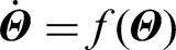
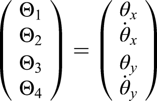
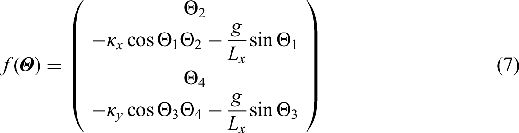
For convenience (7) is labelled as the complete model.

2-Pendulum kinematics

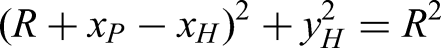
Denoting the location of the pen as (x_H, y_H) it is defined as the intersection of two circles of radius R with centres at (R + x_P, 0) and (0, R + y_P).

(R + x_{P} - x_{H})^{2} + y_{H}^{2} = R^{2}

x_{H}^{2} + (R + y_{p} - y_{H})^{2} = R^{2}

(8)

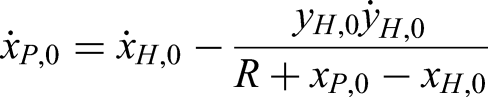
Differentiating (8) with respect to time and dividing by two,

(R + x_{P} - x_{H}) ({\dot{x}}_{P} - {\dot{x}}_{H}) + y_{H} {\dot{y}}_{H} = 0

x_{H} {\dot{x}}_{H} + (R + y_{P} - y_{H}) ({\dot{y}}_{P} - {\dot{y}}_{H}) = 0

(9)

The pendulum conditions can be related to x_P and y_P,

x_{P} = L_{p e} \sin θ_{x}

y_{P} = L_{P} \sin θ_{y}

(10)

Differentiating (10) with respect to time,

{\dot{x}}_{P} = L_{P} \cos θ_{x} {\dot{θ}}_{x}

{\dot{y}}_{P} = L_{P} \cos θ_{y} {\dot{θ}}_{y}

(11)

During the simulation of a harmonograph the pendulum conditions, $(θ_{x}, {\dot{θ}}_{x}, θ_{y}, {\dot{θ}}_{y})$ , are used to calculate (x_H, y_H). Given the pendulum conditions (10) are used to calculate x_P and y_P. The location of the pen (x_H, y_H) is found by solving the nonlinear system,

f (\begin{matrix} x_{H} \\ y_{H} \end{matrix}) = (\begin{matrix} {(R + x_{P} - x_{H})}^{2} + y_{H}^{2} - R^{2} \\ x_{H}^{2} + {(R + y_{p} - y_{H})}^{2} - R^{2} \end{matrix})

(12)

The system is solved using Newton's method,

d_{n} = - J_{n}^{- 1} f_{n}

x_{H, n + 1} = x_{H, n} + d_{n}

(13)

where J_n is the Jacobian of the nonlinear system (12) evaluated at x_H,n . The system (12) depending on x_p, y_p and R has two roots, one root or no roots. For parameters appropriate for a harmonograph there are typically two roots. Fortunately starting with an initial guess for the iteration process as the origin the root closest to the origin is generally found using (13).

Initial conditions for the harmonograph

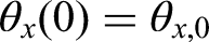
The pendulum initial conditions, $(θ_{x, 0}, {\dot{θ}}_{x, 0}, θ_{y, 0}, {\dot{θ}}_{y, 0})$ must be specified such that the kinematic Equations (8) and (9) are satisfied. To calculate the pendulum initial conditions the initial location of the pen is specified, $(x_{H, 0}, y_{H, 0})$ , the initial location of the top of the pendulums are given by solving (8) for x_P and y_P.

x_{P, 0} = - (R - x_{H, 0}) + \sqrt{R^{2} - y_{H, 0}^{2}}

y_{P, 0} = - (R - y_{H, 0}) + \sqrt{R^{2} - y_{H, 0}^{2}}

(14)

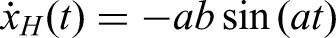
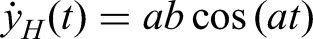
The initial horizontal velocities of the extensions of the two pendulums are also required, see Figure 1. Expressions for the initial velocities, $({\dot{x}}_{P, 0}, {\dot{y}}_{P, 0})$ can be derived by differentiating (14) with respect to time and using (14) to eliminate the square root term, $\sqrt{R^{2} - y_{H, 0}^{2}}$ giving,

{\dot{x}}_{P, 0} = {\dot{x}}_{H, 0} - \frac{y_{H, 0} {\dot{y}}_{H, 0}}{R + x_{P, 0} - x_{H, 0}}

{\dot{y}}_{P, 0} = {\dot{y}}_{H, 0} - \frac{x_{H, 0} {\dot{x}}_{H, 0}}{R + y_{P, 0} - y_{H, 0}}

(15)

see (9). The pendulum initial conditions can then be calculated using (10) and (11).

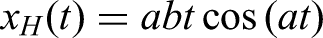
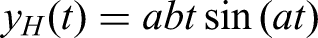
For a harmonograph the device is initiated by the user moving the pen until a picture that is potentially of interest is evolving. The user then releases the pen, and the pendulum dynamics take over the movement of the pen. In the simulations discussed in the next section two parametric curves are explored as geometric pattern initiators. One functional form used to calculate initial conditions for the harmonograph is a circular trajectory.

φ = a t, r = b

x_{H} (t) = b \cos (a t)

y_{H} (t) = b \sin (a t)

{\dot{x}}_{H} (t) = - a b \sin (a t)

{\dot{y}}_{H} (t) = a b \cos (a t)

t \leq t_{r e l}

(16)

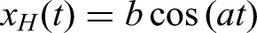
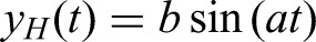
The second set of pendulum initial conditions are calculated using an Archimedean spiral.

φ = a t, r = b φ

x_{H} (t) = a b t \cos (a t)

y_{H} (t) = a b t \sin (a t)

{\dot{x}}_{H} (t) = a b \cos (a t) - a^{2} b t \sin (a t)

{\dot{y}}_{H} (t) = a b \sin (a t) + a^{2} b t \cos (a t)

t \leq t_{r e l}

(17)

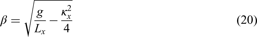
Approximate model for a 2-pendulum harmonograph

If the initial condition is close to the equilibrium point, $(θ_{x}, {\dot{θ}}_{x})_{e q} = (0, 0)$ then the small angle approximation can be invoked, $\sin θ_{x} \approx θ_{x}, \cos θ_{x} \approx 1$ . This gives the approximate model

{\ddot{θ}}_{x} + κ_{x} {\dot{θ}}_{x} + \frac{g}{L_{x}} θ_{x} = 0

(18)

A corollary of the small angle approximation is the kinematics based on (8) and (9) reduce to,

x_{H} = x_{P} = L_{p e} θ_{x}

{\dot{x}}_{H} = {\dot{x}}_{P} = L_{p e} {\dot{θ}}_{x}

(19)

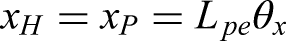
For convenience (18) is labelled as the linear model. The linear model has an analytical solution of the form,

θ_{x} (t) = e^{- α t} (A \sin (β t + \frac{π}{2}) + B \sin (β t))

A, B \geq 0

where

α = \frac{κ_{x}}{2}

β = \sqrt{\frac{g}{L_{x}} - \frac{κ_{x}^{2}}{4}}

(20)

The parameters A and B are determined by the initial conditions. Note if A or B are negative then the phase can be adjusted to make A and B positive.

Simulations of a 2-pendulum harmonograph

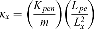
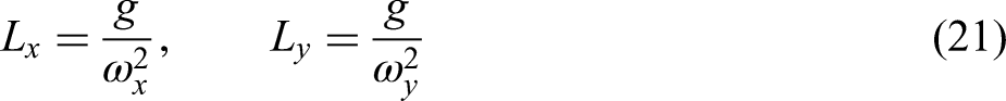
There are many parameters that define the harmonograph. There are too many parameters to comprehensively explore parameter space. Fortunately, there are some physical constraints that define narrow ranges for some parameters. For all simulations unless stated otherwise have the following values: the mass of the pendulum, m = 1 kg, the parameter L_pe = 0.5 m and the rods connected to the pen, R = 0.5 m. The length of the pendulums is specified indirectly by prescribing the natural frequencies.

L_{x} = \frac{g}{ω_{x}^{2}}, L_{y} = \frac{g}{ω_{y}^{2}}

(21)

In a real lateral harmonograph the length of the pendulums is restricted by the physical space available. For a mathematical model this is not an issue. In general, for a harmonograph, the pen resistive force, F_pen is small compared to the weight of the pendulum bobs. In the simulations presented below K_pen is treated as a free parameter. This is equivalent to K_pen being fixed and the importance of the resistive pen force adjusted by increasing or decreasing the mass of the pendulum bob.

Evaluation of the linear model

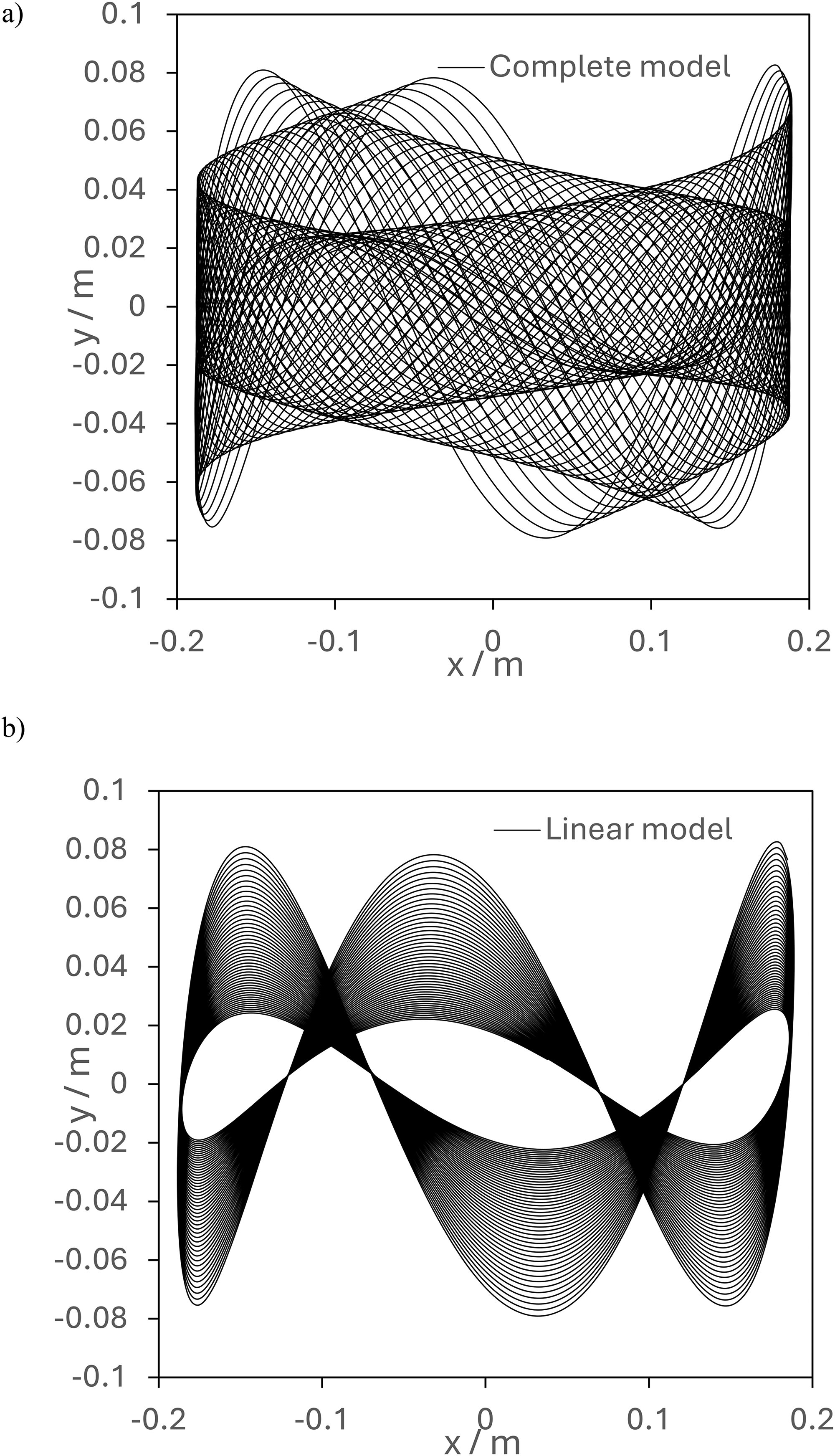
In this subsection the variants of the harmonograph model are compared. Two different harmonograph configurations are considered, Test 1 and Test 2. The two sets of parameter values are given in Table 1. Test 1 is defined primarily by a large value for the resistive pen force coefficient, K_pen = 1. For Test 1 other parameters of note are the frequencies of the pendulums are assigned the values ω_x = ω_y = 2 rad/s. The simulated pen trajectory for the complete model (6), and the linear model (18) are shown in Figure 4. The analytical solution for the linear model applied to the Test 1 conditions is,

x_{H} (t) = e^{- 0.04 t} (0.2 \sin (2 t + \frac{π}{2}) + 0.002 \sin (2 t + π))

y_{H} (t) = e^{- 0.04 t} (0.03 \sin (2 t + \frac{3 π}{2}) + 0.05 \sin (2 t))

(22)

where the constants are given to one significant figure. As the resistive pen force is large, for both the complete model and the linear model the pen follows a spiral trajectory towards the equilibrium point (x_H, y_H) = (0, 0). The complete model prediction and the linear model prediction are very similar. For the Test 1 harmonograph configuration the approximate pen trajectory equations, (2), are valid.

Figure 4.

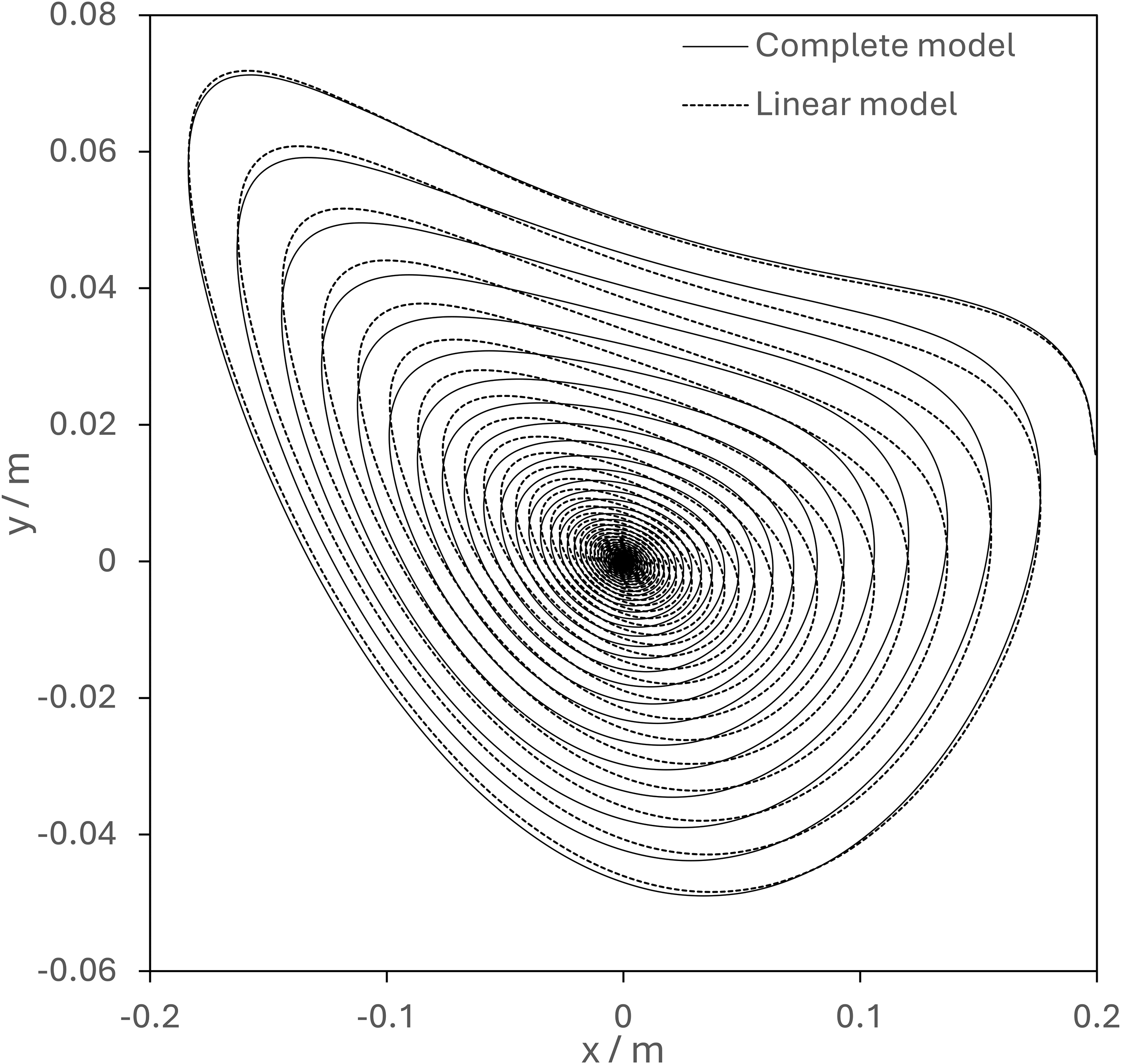
Test 1, geometric design generated.

Table 1.

Simulation conditions.

Test^a	Nu. of Pendulums	ω_x	ω_y	ω_pl	K_pen	R	Initial Condition
Test^a	Nu. of Pendulums	ω_x	ω_y	ω_pl	K_pen	R	Function	a	b	t_rel / s	θ_pl,0
1	2	2	2	–	1	0.5	Circle	0.5	0.2	π/20	–
2	2	1	3	–	0.02	5	Circle	0.5	0.2	π /4	–
3	2	2	2	–	0.1	0.5	Spiral	0.5	0.1	3	–
4	2	2	2	–	0.1	0.5	Spiral	0.5	0.1	5	–
5	2	1.99	2.01	–	0.1	0.5	Spiral	0.5	0.1	3	–
6	2	1.99	2.01	–	0.1	0.5	Spiral	0.5	0.1	5	–
7	2	3.99	1.01	–	0.02	0.5	Circle	3	0.1	7π /4	–
8	2	3.99	1.01	–	0.02	0.5	Circle	6	0.1	7π /4	–
9	3	2	2	2	0.1	0.5	Circle	3	0.1	7π/4	π /4
10	2	2	2	–	0.1	0.5	Circle	3	0.1	7π/4	–
11	3	1.99	2.01	1	0.1	0.5	Circle	3	0.1	7π/4	π /8
12	2	1.99	2.01	–	0.1	0.5	Circle	3	0.1	7π/4	–

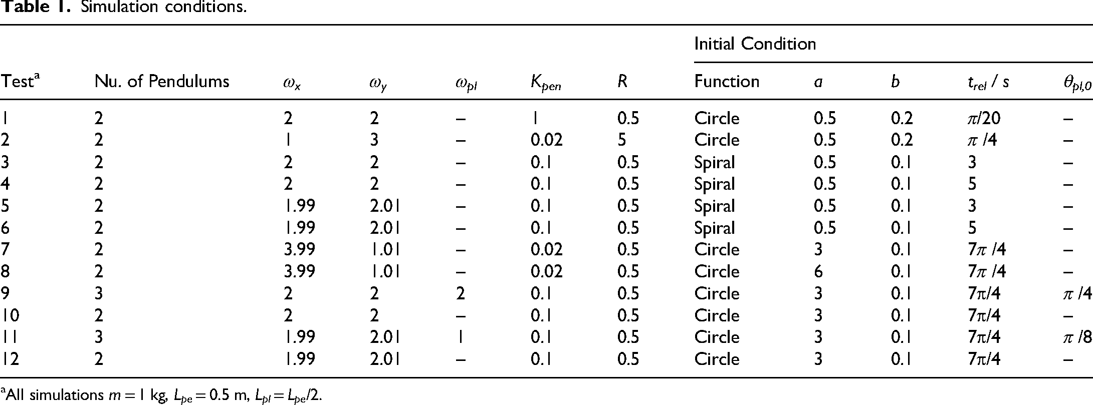
All simulations m = 1 kg, L_pe = 0.5 m, L_pl = L_pe/2.

In Test 2 a set of harmonograph parameter values are specified to give a more interesting geometric shape than a spiral. All parameter values defining Test 2 are given in Table 1. The main parameters defining Test 2 are R = 5 m, K_pen = 0.02 Ns/rad, ω_x = 1 rad/s and ω_y = 3 rad/s. The second test has more initial rotational kinetic energy in the system. Note a connection rod of 5 m would not be possible in most harmonographs but for a mathematical model is possible. Similar to Test 1, two simulations are presented in Figure 5 using the different harmonograph models. Figure 5(a) shows the pen trajectory using the complete model. The effect of the different natural frequencies for the pendulums is clear. The geometric design produced is antisymmetric about the line x = 0 and is far more interesting than a spiral shape. For Test 2 the linear model has an analytical solution of the form,

x_{H} (t) = e^{- 5 \times 10^{- 5} t} (0.2 \sin (t + \frac{π}{2}) + 0.04 \sin (t + π))

y_{H} (t) = e^{- 0.004 t} (0.07 \sin (3 t + \frac{π}{2}) + 0.03 \sin (3 t))

(23)

where the parameter values are stated to one significant figure. The linear model prediction is shown in Figure 5(b) and is qualitatively similar to that shown in Figure 5(a). The two geometric designs shown in Figure 5(a) and (b) have three peaks in the x direction, but quantitatively the trajectories are very different.

Figure 5.

Test 2, geometric design generated.

The overall conclusion of the analysis of Test 1 and Test 2 is that the complete model and the linear model have the potential to produce aesthetically pleasing geometric patterns, but the predicted trajectories calculated by the two models can be very different. The linear model will not be considered further.

Sensitivity to initial conditions

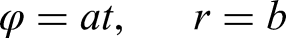
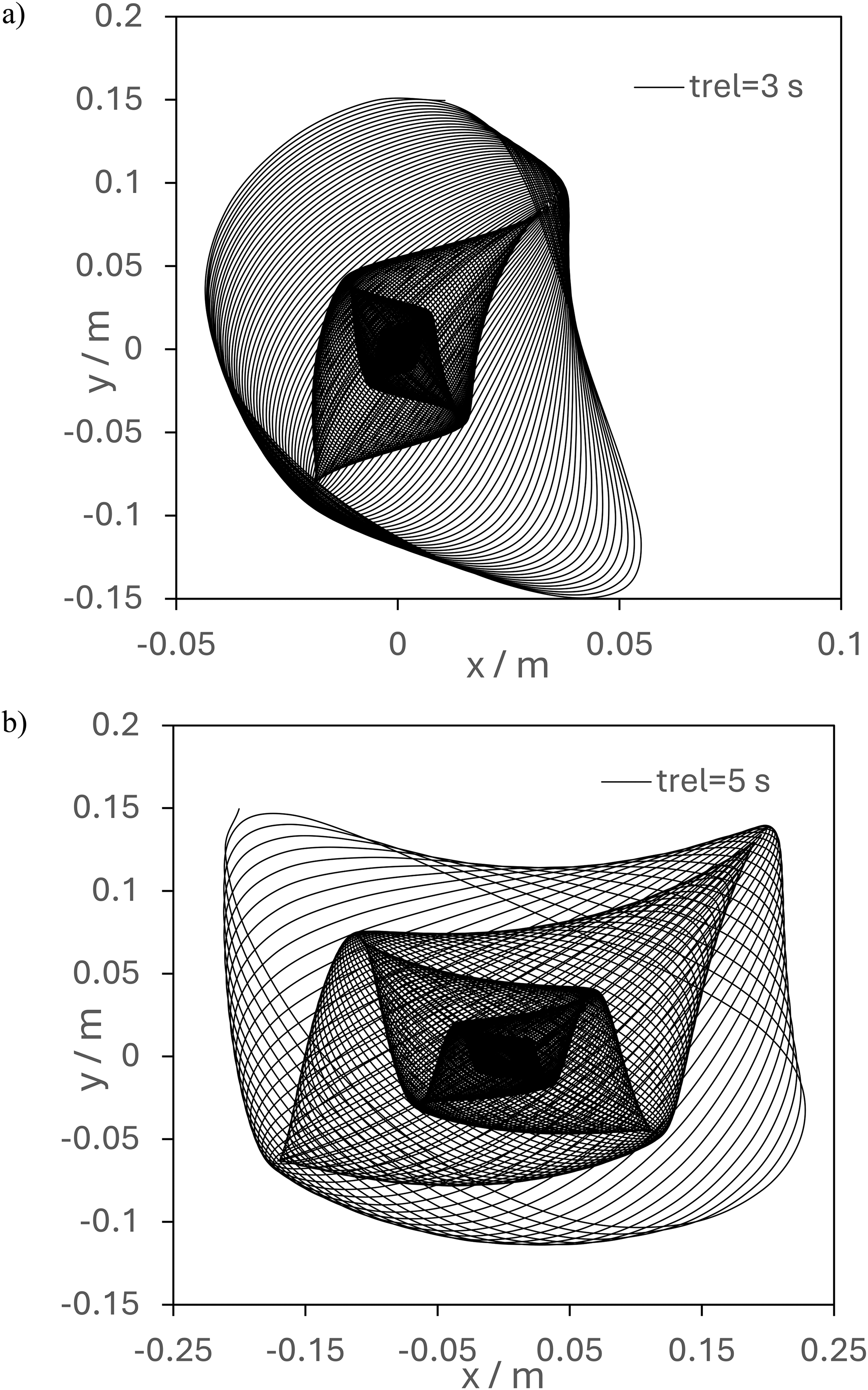
In this subsection the sensitivity of the geometric pattern generated to the initial conditions of the pendulums is investigated. The harmonograph defined in Test 3 and Test 4 are the same as Test 1, the tests differ in the initial conditions specified. In Test 3 and Test 4 the initial conditions of the pendulums are defined by an Archimedean spiral with a = 0.5 and b = 0.1 with a release time of t_rel = 3 s for Test 3 and t_rel = 5 s for Test 4. For both tests the harmonograph pendulums have natural frequencies of ω_x = ω_y = 2 rad/s.

For Test 3 the initial condition specification gives the following initial pendulum conditions.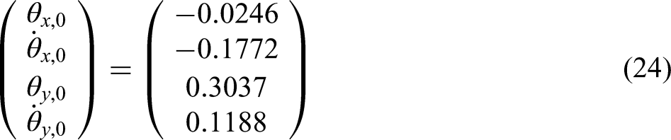

(\begin{matrix} \begin{matrix} θ_{x, 0} \\ {\dot{θ}}_{x, 0} \end{matrix} \\ \begin{matrix} θ_{y, 0} \\ {\dot{θ}}_{y, 0} \end{matrix} \end{matrix}) = (\begin{matrix} \begin{matrix} - 0.0246 \\ - 0.1772 \end{matrix} \\ \begin{matrix} 0.3037 \\ 0.1188 \end{matrix} \end{matrix})

(24)

For Test 4 the initial condition specification gives the following initial pendulum conditions.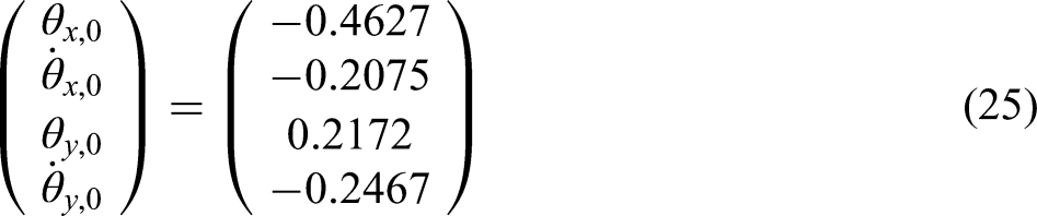

(\begin{matrix} \begin{matrix} θ_{x, 0} \\ {\dot{θ}}_{x, 0} \end{matrix} \\ \begin{matrix} θ_{y, 0} \\ {\dot{θ}}_{y, 0} \end{matrix} \end{matrix}) = (\begin{matrix} \begin{matrix} - 0.4627 \\ - 0.2075 \end{matrix} \\ \begin{matrix} 0.2172 \\ - 0.2467 \end{matrix} \end{matrix})

(25)

The geometric designs generated in Test 3 and Test 4 are shown in Figure 6(a) and (b) respectively. The two patterns are similar in some respects and different in others. For Test 3 the geometric shape resembles a seashell, similar to a mussel. For Test 4 the shape is more complex with the trajectory for early times having a crossing pattern. For later times both patterns asymptote to a straight line of the form, y = mx + c. For Test 3 the gradient m is negative and for Test 4 m is positive. The main difference between the two geometric patterns is the range in x, for Test 3 it is approximately −0.05 < x < 0.05 compared to Test 4 where the range in x is approximately 5 times larger.

Figure 6.

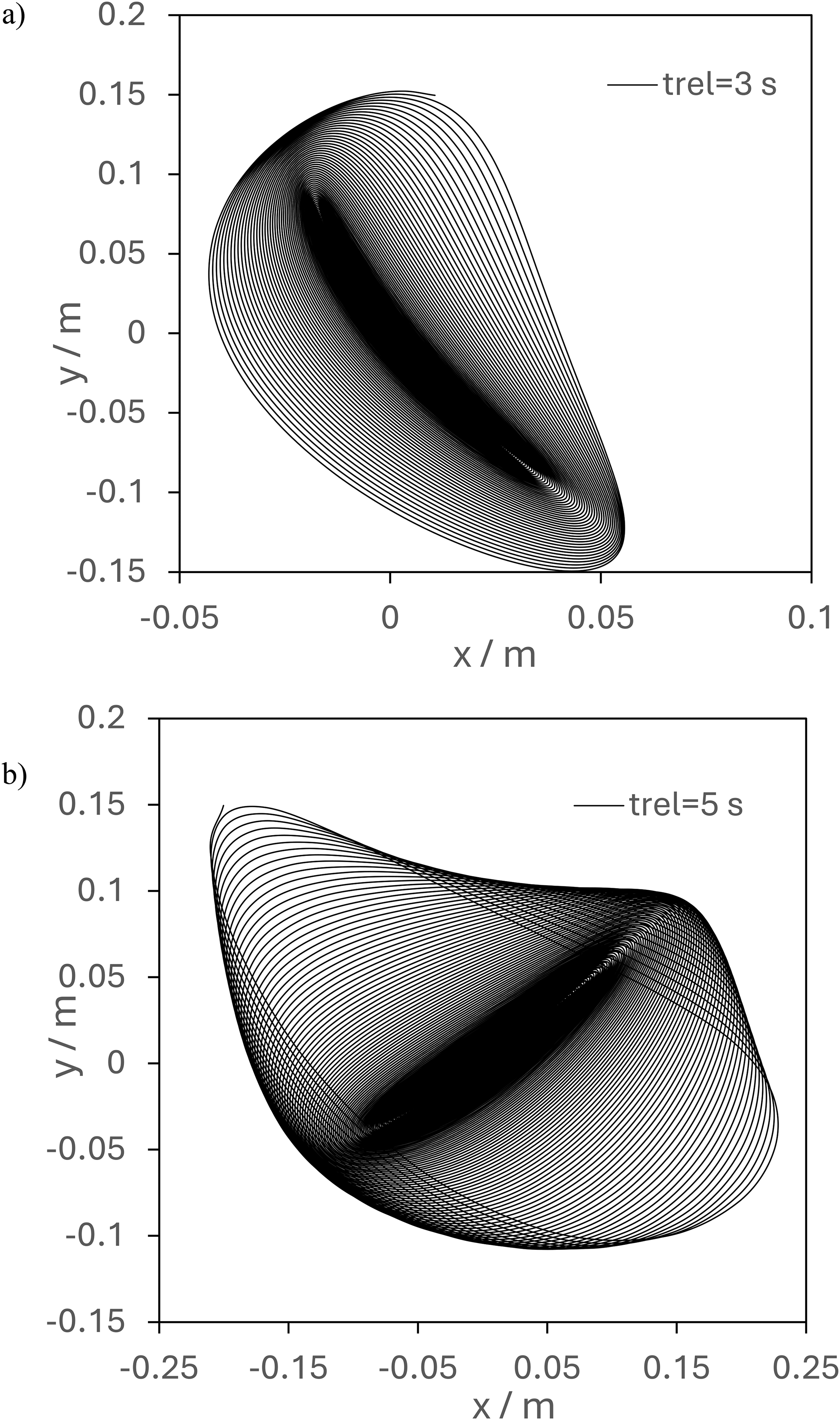
Geometric design generated, (a) Test 3 and (b) Test 4.

Sensitivity to pendulum natural frequency

It is well known by investigators of harmonographs that interesting geometric patterns are possible when the natural frequencies are close to integer values. Test 5 and Test 6 are similar to Test 3 and 4 except the natural frequences are ω_x = 1.99 and ω_y = 2.01. The geometric patterns for Test 5 and Test 6 are shown in Figure 7(a) and (b) respectively. To assess the sensitivity of the geometric pattern produced to the pendulum natural frequencies, Test 5 should be compared to Test 3. The equivalent figures are Figures 7(a) and 6(a). Unsurprisingly the initial trajectory of the pen is similar for both Test 3 and Test 5, but later in the picture generation process the pen trajectories diverge. For Test 3 the trajectory asymptotes to a straight line as discussed above. For Test 5 the situation is much more complex with the geometric pattern producing a series of parallelogram-like shapes centred on the origin that reduce in size and are successively reflected about the y axis.

Figure 7.

Geometric design generated, (a) Test 5 and (b) Test 6.

Comparing Test 6 with Test 4, see Figures 7(b) and 6(b), the range of x and y for the patterns generated is similar. The spacing between the lines for Test 6 are larger than for Test 4, a direct consequence of the small changes in the natural frequencies. Comparing Figure 7(a) and (b), Test 5 and Test 6, the geometric designs have the pattern of reducing area parallelograms with each subsequent parallelogram reflected about the y-axis.

The final two 2-pendulum simulations, Test 7 and Test 8 have the natural frequencies ω_x = 3.99 rad/s and ω_y = 1.01 rad/s. The initial conditions for the geometric pattern generation are a circular trajectory where Test 7 has an initial angular velocity of 3 rad/s and Test 8 has an initial angular velocity of 6 rad/s. For Test 7 the initial condition specification gives the following initial pendulum conditions.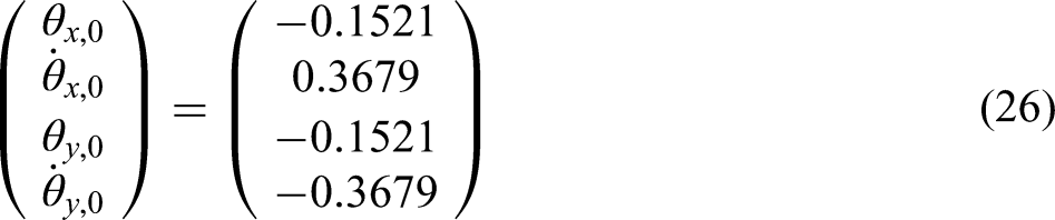

(\begin{matrix} \begin{matrix} θ_{x, 0} \\ {\dot{θ}}_{x, 0} \end{matrix} \\ \begin{matrix} θ_{y, 0} \\ {\dot{θ}}_{y, 0} \end{matrix} \end{matrix}) = (\begin{matrix} \begin{matrix} - 0.1521 \\ 0.3679 \end{matrix} \\ \begin{matrix} - 0.1521 \\ - 0.3679 \end{matrix} \end{matrix})

(26)

The geometric pattern generated is shown in Figure 8(a). The pattern produced resembles a ribbon with several twists in it. The pen trajectory asymptotes to a near vertical line before tending to the equilibrium point (x_H, y_H) = (0, 0). The trajectory asymptoting to a near vertical line is one consequence of the different pendulum natural frequencies as the resistive coefficient parameter κ_y is less than κ_x, see (6).

Figure 8.

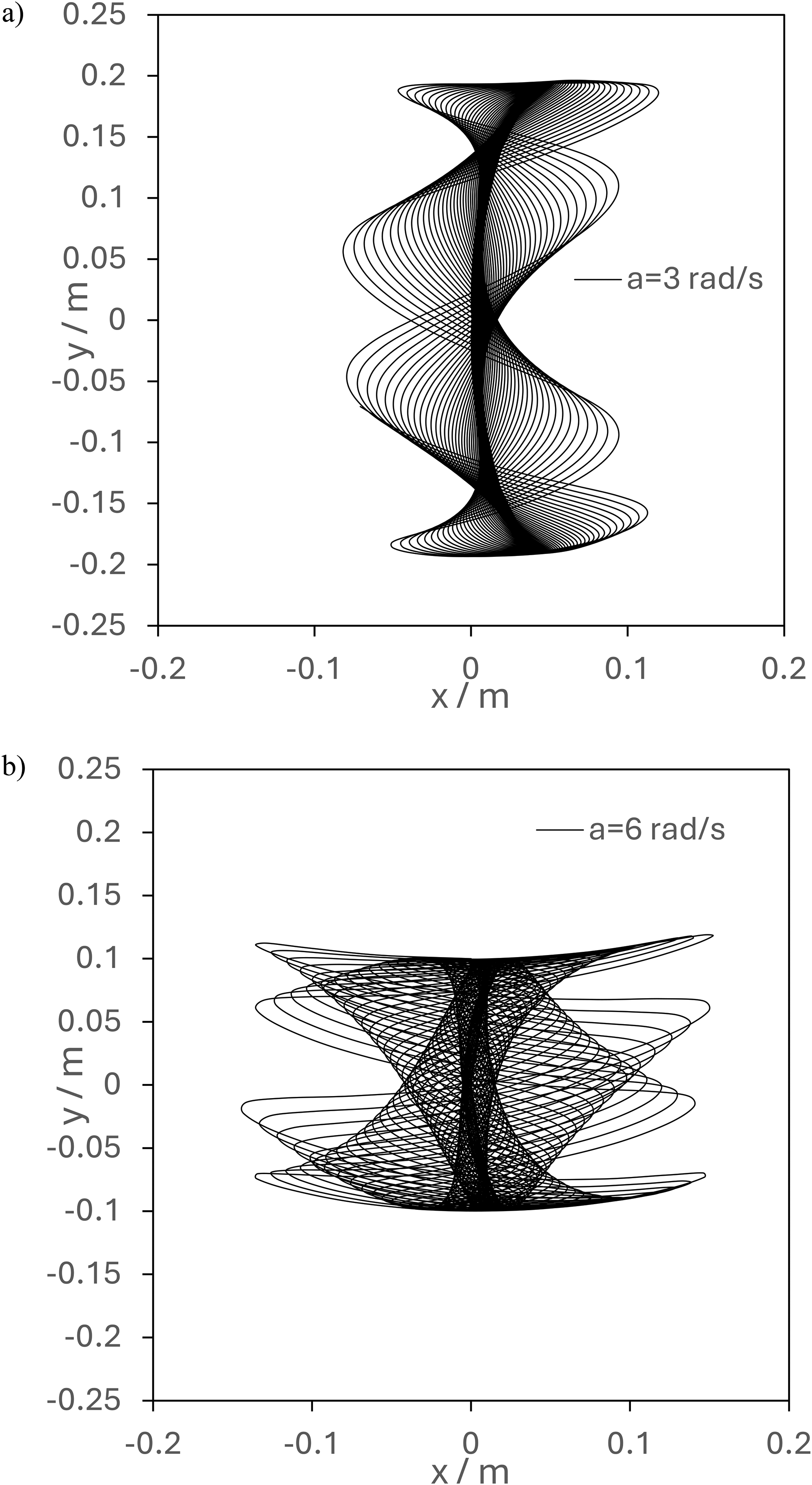
Geometric design generated, (a) Test 7 and (b) Test 8.

For Test 8 the initial condition specification gives the following initial pendulum conditions.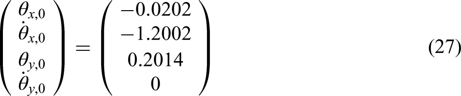

(\begin{matrix} \begin{matrix} θ_{x, 0} \\ {\dot{θ}}_{x, 0} \end{matrix} \\ \begin{matrix} θ_{y, 0} \\ {\dot{θ}}_{y, 0} \end{matrix} \end{matrix}) = (\begin{matrix} \begin{matrix} - 0.0202 \\ - 1.2002 \end{matrix} \\ \begin{matrix} 0.2014 \\ 0 \end{matrix} \end{matrix})

(27)

For Test 8, when the pen is released, it has twice the velocity of Test 7. The geometric design produced is shown in Figure 8(b). Comparing Figure 8(b) with 8(a) the design is topologically very similar except the range of y_H is reduced and the range of x_H is increased. The overall appearance in Figure 8(b) is a ‘squashed’ version of the geometric pattern shown in Figure 8(a).

It is difficult to predict the geometric pattern generated when changing the parameters defining the harmonograph and pen release conditions. When using the mathematical model of a harmonograph to generate interesting geometric designs, it is a case of numerical experimentation, adjusting parameters that define the harmonograph and initial pen trajectory. This is much like a mechanical harmonograph.

3-Pendulum harmonograph

The 2-pendulum harmonograph can produce interesting geometric designs, but even more complex geometric patterns are possible with a 3-pendulum or 4-pendulum harmonograph. Considering a 3-pendulum harmonograph further, the additional harmonic motion is introduced by oscillating the platform the paper is placed on. The platform can be oscillated directly such that the platform undergoes angular motion, see Figure 9(a). In an alternative 3-pendulum design the platform is on wheels guided by tracks, or the platform is suspended. For the wheeled platform design, the platform has a connecting rod to the oscillating pendulum, see Figure 9(b). The platform undergoes horizontal oscillating motion. As to which type of 3-pendulum harmonograph is the better? The directly driven platform oscillation harmonograph is the simplest to fabricate. As far as the mathematical basis for a 3-pendulum harmonograph model, the wheeled platform harmonograph is the simpler extension of the 2-pendulum harmonograph model.

Figure 9.

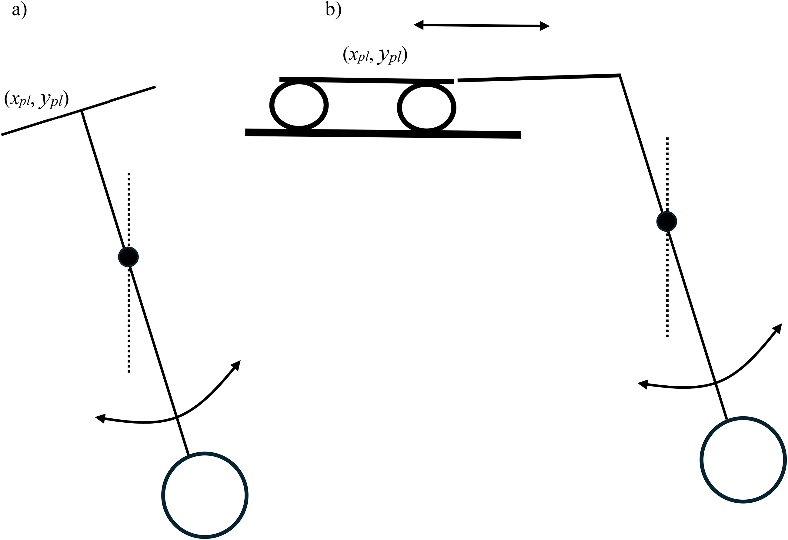
Platform motion in a 3-pendulum harmonograph, (a) direct drive and (b) indirect drive.

3-Pendulum model

We will present a 3-pendulum harmonograph based on the horizontal oscillating platform design, see Figure 9(b). For the 3-pendulum harmonograph the dynamics of the pen is similar to a 2-pendulum harmonograph except the movement of the platform must be accounted for.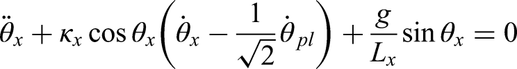

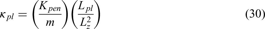
{\ddot{θ}}_{x} + κ_{x} \cos θ_{x} ({\dot{θ}}_{x} - \frac{1}{\sqrt{2}} {\dot{θ}}_{p l}) + \frac{g}{L_{x}} \sin θ_{x} = 0

{\ddot{θ}}_{y} + κ_{y} \cos θ_{y} ({\dot{θ}}_{y} - \frac{1}{\sqrt{2}} {\dot{θ}}_{p l}) + \frac{g}{L_{y}} \sin θ_{y} = 0

(28)

The dynamics of the pendulum driving the motion of the platform is similar to the pendulums used to drive the pens motion, a moment is taken about the pivot and Newton's second law is applied.

I {\ddot{θ}}_{p l} = - m g L_{z} \sin θ_{p l} - T_{f r i c} - F_{p e n} L_{p l} \cos θ_{p l}

(29)

Using the same assumptions, such as the pendulum bob is a point mass and the frictional torque at the pivot is negligible, and taking platform motion to be on the identity line y = x, gives a simplification of the model.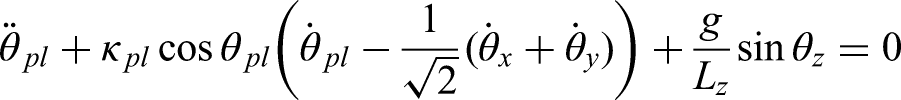

{\ddot{θ}}_{p l} + κ_{p l} \cos θ_{p l} ({\dot{θ}}_{p l} - \frac{1}{\sqrt{2}} ({\dot{θ}}_{x} + {\dot{θ}}_{y})) + \frac{g}{L_{z}} \sin θ_{z} = 0

κ_{p l} = (\frac{K_{p e n}}{m}) (\frac{L_{p l}}{L_{z}^{2}})

(30)

The location of the centre of the platform is,

x_{p l} = y_{p l} = \frac{1}{\sqrt{2}} L_{p l} \sin θ_{p l}

(31)

The location of the pen relative to the centre of the paper is,

x_{p l, H} = x_{H} - x_{p l}

y_{p l, H} = y_{H} - y_{p l}

(32)

Simulations of a 3-pendulum harmonograph

In this section only two simulations of a 3-pendulum harmonograph are considered. For Test 9 the initial condition of the pendulum driving the motion of the platform is it is stationary with an orientation,

θ_{p l, 0} = \frac{π}{4} r a d

(33)

In Test 9 the natural frequencies of all three pendulums are set to ω_x = ω_y = ω_pl = 2 rad/s. The pattern generated is shown in Figure 10(a). The geometric pattern produced is similar to a projection of a collection of tori one inside another. The tori are aligned with the identity line y = x. The impact of the platform oscillations can be appreciated by comparing Test 9 and Test 10. Test 10 has the same set of harmonograph conditions except the platform is stationary, see Table 1. This means Test 10 is a 2-pendulum simulation. Figure 10(b) shows the geometric design generated for Test 10, which resembles a slowly decaying spiral. The geometric design produced for Test 9, shown in Figure 10(a) is radically different from Test 10, but the only difference in setup of the harmonograph is the decaying oscillation of the platform, in Test 9, or stationary condition of the platform, in Test 10.

Figure 10.

Geometric design generated, (a) Test 9 and (b) Test 10.

The final pair of simulations considered are Test 11 and Test 12. For Test 11 the natural frequencies of the three pendulums are, ω_x = 1.99 rad/s, ω_y = 2.01 rad/s and ω_pl = 1 rad/s. The platform pendulum is initially stationary with an orientation,

θ_{p l, 0} = \frac{π}{8} r a d

(34)

For Test 11, the geometric pattern generated is shown in Figure 11(a). The geometric picture is complex making it difficult to characterise. It is an interesting design and is aesthetically pleasing. This demonstrates that similar to the 2-pendulum harmonograph, natural frequency's close to integer values are interesting regions of parameter space to explore. For comparison purposes the 2-pendulum simulation with the natural frequencies, ω_x = 1.99 rad/s, ω_y = 2.01 rad/s, Test 12 is shown in Figure 11(b). Figures 10 and 11 demonstrate the extension of the range of geometric pattern generation possible with the introduction of the third pendulum.

Figure 11.

Geometric design generated, (a) Test 11 and (b) Test 12.

The investigation of harmonographs with natural frequencies close to integer values has an impact on the practical design of harmonographs as it is almost impossible to give a pendulum an exact integer value for its natural frequency as experimental error and precision comes into play.

Using the harmonograph models to enhance the student experience

The harmonograph models can be used to reinforce and support pendulum analysis in introductory and intermediate dynamics courses for undergraduate engineering students. The harmonograph is a memorable example of a dynamic model where the interplay between natural frequencies of multiple pendulums and frictional losses produces interesting behaviour. The author has used the software based on the harmonograph models presented in this paper to enthuse undergraduate 1st year students taking introductory courses in dynamics. The harmonograph simulations have been produced in lectures once the dynamics of a pendulum has been presented.

The MATLAB implementation of the harmonograph models are relatively straightforward to produce with very little programming knowledge. A block diagram of the MATLAB harmonograph model software is shown in the Appendix. The 2-pendulum harmonograph MATLAB software is available on request to the author. At present the model simulation set up is changed by editing a MATLAB script. Ultimately a GUI for the harmonograph models would be a useful extension of the software. The parameter space defining the harmonograph and initial conditions of the pen and platform invite engineering students to explore the behaviour of harmonographs by numerical experimentation using the MATLAB software.

One of the interesting points of a geometric design produced by a mechanical harmonograph, is the observation of the evolution of the geometric design can be viewed in real time. There is a similar possibility in MATLAB where the trajectory of the pen and the evolution of the pattern produced can be shown using the MATLAB function, comet, in place of the plot function. In a paper the evolution of a harmonograph design can only be partially demonstrated by showing a geometric design at certain times. As an example of this, the geometric design produced for Test 11 is shown in Figure 12. In Figure 12 the geometric design for Test 11 is produced for t = 30 s, Figure 12(a), t = 60 s, Figure 12(b), t = 120 s, Figure 12(c), and t = 240 s, Figure 12(d). Considering Figure 12 as a whole it is clear that with increasing time the geometric pattern produced changes in a way that is almost impossible to determine apriori.

Figure 12.

Evolution of a geometric design for test 11, (a) t = 30 s, (b) t = 60 s, (c) t = 120 s and (d) t = 240 s.

Conclusion

In this paper a model for a 2-pendulum lateral harmonograph and a 3-pendulum lateral harmonograph derived from first principles are presented. The model derivation uses concepts such as free body diagrams, mass acceleration diagrams and kinematic equations typically introduced in introductory and intermediate university courses in dynamics. A number of geometric designs generated by the harmonograph models are analysed. It is demonstrated that the geometric pattern produced is sensitive to the initial conditions and parameters defining the harmonograph. There are an infinite number of geometric designs that the harmonograph models can generate and this paper gives a small insight into what is possible.

The harmonograph models presented here represent the beginning of an investigation into what is possible when it comes to the mathematical modelling of harmonographs and the use of such models to encourage engagement of undergraduate students with dynamics. This paper demonstrates that a relatively simple system, the simple pendulum can demonstrate diverse dynamic behaviour. A perspective of some undergraduate mechanical engineering students is that the dynamic behaviour of a pendulum is boring. This paper challenges this attitude.

How could the models presented here be extended? It is relatively straightforward to apply first principles to a 4-pendulum harmonograph in a similar way to the derivation of the 2-pendulum lateral harmonograph and the 3-pendulum lateral harmonograph. It is a bigger step to apply similar modelling techniques to derive a model for a rotary harmonograph but deriving such a model would be a useful thing to do.

To give the harmonograph models to a student cohort and let the students discover what is possible for themselves is an attractive option, but student empowerment would be enabled further by developing a GUI for the harmonograph models. As it stands the MATLAB software can be given to the student cohort for them to explore parameter space with minimal supervision. The harmonograph models presented here have a large potential to enhance the student experience making the student cohort more readily engage with a mechanical engineering science, dynamics that in the past students have perceived as a course to be endured rather than enjoyed.

Footnotes

ORCID iD

Peter S Cumber

Funding

The author received no financial support for the research, authorship, and/or publication of this article.

Declaration of conflicting interests

The author declared no potential conflicts of interest with respect to the research, authorship, and/or publication of this article.

Data availability statement

Data sharing not applicable to this article as no datasets were generated or analyzed during the current study.

Appendix – Block diagram for MATLAB implementation. *ode45 – predefined MATLAB function. A copy of the MATLAB software for a 2-pendulum harmonograph can be obtained from the author.

References

Berry

Savage

Williams

. Mechanics in decline? Int J Math Educ Sci Technol 1989; 20: 289–296.

Biggoggero

Rovida

. Problems in the teaching of mechanics. Eur J Eng Educ 1977; 2: 277–290.

Firouzian

Ismail

Abd Rahman

, et al. Mathematical competency of engineers and engineering students. In: 2014 international conference on teaching and learning in computing and engineering, 2014, pp.216–219. doi https://doi.org/10.1109/LaTiCE32374.2014.

Piepin

Bichler

Gueudet

. Mathematics in engineering education: A review of the recent literature with a view towards innovative practices. Int J Res Undergrad Math Educ 2021; 7: 163–188.

Graham

Peek

. Developing an approach to the introduction of rigid body dynamics. Int J Math Educ Sci Technol 1997; 28: 373–380.

Graham

Rowlands

. Using computer software in the teaching of mechanics. Int J Math Educ Sci Technol 2000; 31: 479–493.

Wideberg

. A graphical user interface for the learning of lateral vehicle dynamics. Eur J Eng Educ 2003; 28: 225–235.

Cumber

. Waggling pendulums and visualisation in mechanics. Int J Math Educ Sci Technol 2015; 46: 611–630.

Fay

. The pendulum equation. Int J Math Educ Sci Technol 2002; 33: 505–519.

10.

Bevivino

. The path from the simple Pendulum to chaos, Colorado state university. Dyn Horsetooth 2009; 1: 1–24.

11.

Big-Alabo

. Approximate periodic solution for the large-amplitude oscillations of a simple pendulum. Int J Mech Eng Educ 2020; 48: 335–350.

12.

Stein

Parcic

Singh

. From playground swings to sway control of cranes: An active pendulum experiment. Int J Mech Eng Educ 2023; 51: 139–154.

13.

Cumber

. Waggling conical pendulums and visualisation in mechanics. Int J Math Educ Sci Technol 2016; 47: 612–636.

14.

Cumber

. Lagrange’s method applied to a slinky. Int J Mech Eng Educ 2024; 52: 372–400.

15.

Cumber

. Complete dynamic model of a Slinky based on torsion springs. Int J Mech Eng Educ 2024. https://doi.org/10.1177/03064190241293025

16.

Crowell

. Motion of the earth as viewed from the moon and the Y-suspended pendulum. Am J Phys 1981; 49: 452–454.

17.

Whitaker

. A note on the blackburn pendulum. Am J Phys 1991; 59: 330–333.

18.

Steckenrider

Adaptive aerial localization using Lissajous search patterns. IEEE Trans Robot 2022; 38: 2094–2113.

19.

Sierra

. Recurrence in Lissajous Curves and the Visual Representation of Tuning Systems. Found Sci 2023. https://doi.org/10.1007/s10699-023-09930-z

20.

Fay

Graham

. Coupled spring equations. Int J Math Educ Sci Technol 2003; 34: 65–79.

21.

Anurakpandit

Townsend

Wilson

. The numerical and experimental investigations of a gimballed pendulum energy harvester. Int J Non-Linear Mech 2020; 120: 103384.

22.

Whitaker

. Harmonographs. I. Pendulum design. Am J Phys 2001; 69: 162–173.

23.

Whitaker

. Harmonographs. II. Circular design. Am J Phys 2001; 69: 174–183.

24.

Pastor

Obradovic

Kojic

. Combination of perpendicular oscillations and analysis of harmonograph’s curves using math and CAD tools. In: Conference 2nd international scientific conference on geometry and graphics moNGeometrija Belgrade, Serbia, 2010. doi https://doi.org/10.13140/2.1.1440.0323.

A mathematical model for a lateral harmonograph

Abstract

Keywords

Introduction

2-Pendulum harmonograph model

Simple pendulum model

2-Pendulum kinematics

Initial conditions for the harmonograph

Approximate model for a 2-pendulum harmonograph

Simulations of a 2-pendulum harmonograph

Evaluation of the linear model

Sensitivity to initial conditions

Sensitivity to pendulum natural frequency

3-Pendulum harmonograph

3-Pendulum model

Simulations of a 3-pendulum harmonograph

Using the harmonograph models to enhance the student experience

Conclusion

Footnotes

ORCID iD

Funding

Declaration of conflicting interests

Data availability statement

Appendix – Block diagram for MATLAB implementation. *ode45 – predefined MATLAB function. A copy of the MATLAB software for a 2-pendulum harmonograph can be obtained from the author.

References