A mathematical model for a rotary harmonograph

Abstract

In this paper a mathematical model for a rotary harmonograph with two or three pendulums is presented. The rotary harmonograph model is derived using first principles and is a complete model in the sense that it includes the equations of motion, the kinematic expressions relating the pen trajectory to the pendulum conditions, and a prescription of harmonograph initial conditions that mimics the way a physical harmonograph is initiated. The rotary harmonograph model is used to generate a number of geometric designs for the 2-pendulum and 3-pendulum harmonograph. The sensitivity of the geometric design produced to the natural frequencies, friction and pendulum initial conditions is investigated. The generated patterns are qualitatively similar to the output of physical harmonographs.

Introduction

The dynamics of pendulums is very interesting, the trouble is, convincing undergraduate mechanical engineering students that this is the case can be a problem. ¹ This paper is one of a series that are focussed on using mechanical systems to engage with engineering undergraduates. The message is, there is value in investigating pendulum dynamics. An engineering or physics undergraduate is introduced to a simple pendulum early in their university education, typically the concept of resonance, the forcing of a pendulum at its natural frequency is presented and the investigation stops there. This paper shows an example of pendulum dynamics that demonstrates the topic of pendulum dynamics is so much more than resonance. The motivation for this investigation is to show that pendulum dynamics can be both interesting and beautiful.

A harmonograph is a mechanical drawing device that can generate interesting geometric patterns.^2,3 The moving parts of a harmonograph are driven by two or more pendulums. One or two pendulums are connected to a pen that rests on a piece of paper on a platform. The platform can be fixed, or it can be driven by a pendulum to rotate using a conical pendulum or undergo harmonic motion under the action of a simple pendulum.

Previously a mathematical model derived from first principles for a 2-pendulum or 3-pendulum lateral harmonograph based on simple pendulums, has been published. ⁴ This paper presents a mathematical model for a 2-pendulum rotary harmonograph and a 3-pendulum rotary harmonograph based on conical pendulums. A rotary harmonograph is a more challenging device to model compared to a lateral harmonograph. A rotary harmonograph produces geometric pictures that are 2-dimensional projections of up to a 12-dimensional phase space. For many areas of parameter space defining the harmonograph and its initial conditions the 2-dimensional projection is a space filling curve that is not very interesting, but for other regions of parameter space the drawing produced by the harmonograph has a beautiful structure that is aesthetically pleasing.

Literature review

The first device based on a pendulum that produces geometric designs is a pendulum called a Blackburn pendulum, invented in 1815 by James Dean and reinvented in 1844 by Hugh Blackburn. ⁵ A Blackburn pendulum can produce 2-dimensional patterns as the pendulum bob is suspended on a Y-shaped line. This means that the pendulum can oscillate in two directions at the same time. It has been recognised that 2-dimensional pendulums have a place in education. ⁶

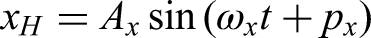
In the open literature research related to harmonographs is mostly focussed on physical harmonographs and their construction. Whitaker,^3,4 discusses the historical development of different types of physical harmonographs. There is a sparsity of papers on the modelling of harmonographs. A mathematical model for a lateral harmonograph derived using first principles is analysed in. ⁴ Other research related to harmonographs are investigations of Lissajous curves.^7–9 Lissajous curves take the form,

$$x_H=A_x\sin ({\omega }_{x}t+p_x)$$

$$y_H=A_y\sin ({\omega }_{y}t)$$

(1)

Lissajous curves can be linked with the theory of music and harmonics.^7,8 Different mechanisms for producing Lissajous curves are discussed in. ⁹ An unusual application of Lissajous curves is the investigation of Lissajous curves as a basis for producing aerial search patterns. ¹⁰

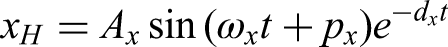
An empirical extension of Lissajous curves to a curve that might be generated by a harmonograph takes the form, ¹¹

$$x_H=A_x\sin ({\omega }_{x}t+p_x)e^{-d_{x}t}$$

$$y_H=A_y\sin ({\omega }_{y}t+p_y)e^{-d_{y}t}$$

(2)

where the decay constants, d_x and d_y introduce the effect of the frictional loss due to the motion of the pen on the platform of the harmonograph. ¹² The geometric patterns produced by (2) should be considered “harmonograph like” as it is not possible to take parameter values in (2) and relate it directly to a harmonograph and prescribed initial conditions for a harmonograph. The empirical harmonograph model (2) are solutions to the linearised simple pendulum model. ⁴ The linearised simple pendulum model is valid for small angle displacements of the azimuthal angle, but this has no relevance to a conical pendulum. ¹³ In ⁴ an evaluation of (2) as an approximation to a lateral harmonograph showed that for only a small region of parameter space is the approximate trajectory similar to the complete model pen trajectory. The approximate model and the complete model of a lateral harmonograph produce similar pen trajectories when the frictional losses are sufficiently large that the pen trajectory produces a spiral like curve centred on the origin.

In this paper a mathematical model for a rotary harmonograph based on first principles is derived and investigated. The initial conditions for the rotary harmonograph are generated in a way that mimics a physical harmonograph. As part of the model the kinematics for a rotary harmonograph are presented.

2-Pendulum harmonograph model

In this section the equations of motion and associated kinematic relations for a 2-pendulum rotary harmonograph are presented. The basis of rotary harmonographs is the conical pendulum. ¹³

Conical pendulum model

A schematic diagram of a conical pendulum where the pendulum is suspended from a horizontal boom, B is given in Figure 1. Figure 1 also shows the weight acting through the centre of mass of the pendulum bob and the tension, T acting through the weightless connecting rod. Note for the remainder of the paper T will denote the kinetic energy of the system, see below.

Figure 1.

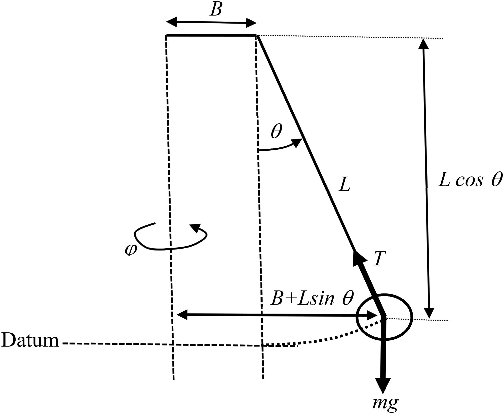
Conical pendulum with a boom.

Initially we consider a conical pendulum without a boom, B = 0, see Figure 1. A conical pendulum is a two degrees of freedom model with independent variables the azimuthal angle, φ, and the polar angle, θ. The pendulum bob is treated as a point mass, m. The conical pendulum is taken to be an undamped system, so drag and friction at the pivot are assumed to be negligible. In, ¹³ the equations of motion for a forced conical pendulum are derived using Newtonian laws of motion. For the undamped conical pendulum, the same approach can be used but one based on the Lagrangian is simpler to formulate. The Lagrangian is defined to be,

$$\mathcal{L}=T-V$$

(3)

Where T is the kinetic energy of the system and V is the potential energy of the system.

$$T={\displaystyle \frac{1}{2}{I}_{\theta }{\dot{\theta }}^2+{\displaystyle \frac{1}{2}{I}_{\phi }{\dot{\phi }}^2}}$$

$$V=mgL(1-\cos \theta )$$

(4)

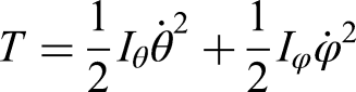
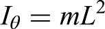
Figure 1 shows the important lengths and symbols used to define the kinetic energy and potential energy expressions given above. In the initial analysis given below the horizontal boom, B is set to zero. The mass moment of inertias, I_θ and I_φ can be expressed as,

$$I_{\theta }=m{L}^2$$

$$I_{\phi }=m{L}^2{\sin }^2\theta$$

(5)

The equations of motion for the conical pendulum are then given by,

$${\displaystyle \frac{d}{dt}\left[{\displaystyle \frac{\mathrm{\partial }\mathcal{L}}{\mathrm{\partial }\dot{\theta }}}\right]-{\displaystyle \frac{\mathrm{\partial }\mathcal{L}}{\mathrm{\partial }\theta }=0}}$$

$${\displaystyle \frac{d}{dt}\left[{\displaystyle \frac{\mathrm{\partial }\mathcal{L}}{\mathrm{\partial }\dot{\phi }}}\right]-{\displaystyle \frac{\mathrm{\partial }\mathcal{L}}{\mathrm{\partial }\phi }=0}}$$

(6)

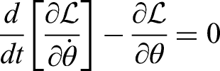
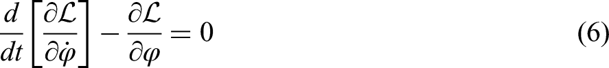
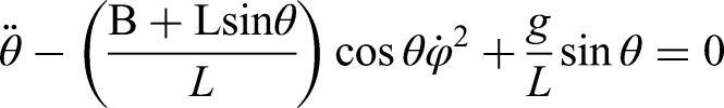
Making the substitutions for the mass moments of inertia into (4) and differentiating the different terms in the Lagrangian gives the equations of motion for a conical pendulum.

$$m{L}^2\ddot{\theta }-m{L}^2\sin \theta \cos \theta {\dot{\phi }}^2+mgL\sin \theta =0$$

$$m(L\sin \theta {)}^2\ddot{\phi }+2m{L}^2\sin \theta \cos \theta \dot{\theta }\dot{\phi }=0$$

(7)

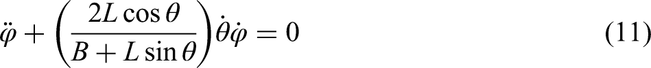
These equations can be derived by taking moments about the two axes of rotation and applying Newtons 2^nd law of motion, but the analysis is more complicated. These equations can be simplified further to give,

$$\ddot{\theta }-\sin \theta \cos \theta {\dot{\phi }}^2+{\displaystyle \frac{g}{L}\sin \theta =0}$$

$$\ddot{\phi }+{\displaystyle \frac{2}{\tan \theta }\dot{\theta }\dot{\phi }=0}$$

(8)

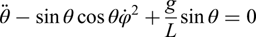
For a simple pendulum there is some value to investigating the small angle approximation, sin θ ≈ θ and cos θ≈1, but for a conical pendulum it is not possible to take a small angle analysis forward to the point an analytical solution can be found.

If the angular velocity, $\dot{\phi }$ , in (8) is taken to be constant then θ is also constant and the equations of motion reduce to,

$$\dot{\phi }=\sqrt{{\displaystyle \frac{g}{L\cos \theta }}}$$

(9)

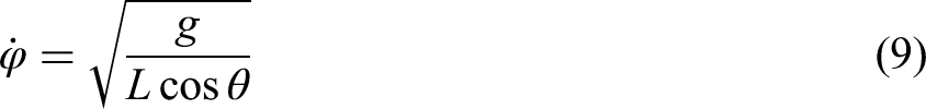
The classic relationship between angular velocity, $\dot{\phi }$ and azimuthal angle, θ for a conical pendulum.

For θ = 0 the system has a singularity but is not an issue unless frictional losses are introduced into the model. This problem can be avoided by changing the case to a conical pendulum with a horizontal boom between the pivot and the axis of rotation, see Figure 1. The horizontal boom changes the mass moment of inertia to,

$$I_{\phi }=m(B+L\sin \theta {)}^2$$

(10)

where B is the length of the horizontal boom. Substituting this into the kinetic energy term T and differentiating the Lagrangian as required the system of equations for this type of conical pendulum is,

$$\ddot{\theta }-\left({\displaystyle \frac{\mathrm{B}+\mathrm{Lsin}\theta }{L}}\right)\cos \theta {\dot{\phi }}^2+{\displaystyle \frac{g}{L}\sin \theta =0}$$

$$\ddot{\phi }+\left({\displaystyle \frac{2L\cos \theta }{B+L\sin \theta }}\right)\dot{\theta }\dot{\phi }=0$$

(11)

For practical purposes B can be made small but finite to model the motion of a rotary harmonograph.

Extension of the conical pendulum model

In this subsection the extension of a conical pendulum to a rotary harmonograph is considered. Figure 2 shows a schematic diagram for a 2-pendulum rotary harmonograph. One conical pendulum is attached to the pen, and a second controls the motion of the platform. The rotational motion is achieved by the pivot being two gimbals connected to allow motion in two dimensions. For a rotary harmonograph the light rod connecting the pendulum bob to the pivot extends beyond the pivot.

Figure 2.

A schematic diagram of a 2-pendulum rotary harmonograph.

The two pendulums act independently apart from there is a resistive force that damps both pendulums due to the motion of the pen on the paper. The force has a small magnitude but can have an impact on the geometric design generated. The relative magnitude of the resistive force is controlled by the mass of the pendulum bobs, m. If m is large, then the resistive force has a smaller impact on the dynamics of the pen and platform.

Starting from the undamped model equations for a single conical pendulum (11), and introducing the resistive force gives a system of equations for the pendulum driving the pen,

$$m{L}_{px}^2{\ddot{\theta }}_{px}-m{L}_{px}(B+L_{px}\sin {\theta }_{px})\cos {\theta }_{px}{\dot{\phi }}_{px}^2+mg{L}_{px}\sin {\theta }_{px}+F_{px,\theta }{L}_{px,2}\cos {\theta }_{px}=0$$

$$\begin{array}{rl}m(& B+L_{px}\sin {\theta }_{px}{)}^2{\ddot{\phi }}_{px}+2m{L}_{px}(B+L_{px}\sin {\theta }_{px})\cos {\theta }_{px}{\dot{\theta }}_{px}{\dot{\phi }}_{px}\\ & +F_{px,\phi }{L}_{px,2}\sin {\theta }_{px}=0\end{array}$$

(12)

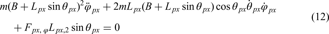
F_px,θ and F_px,φ are components of the resistive force between the motion of the pen and platform. The model for the conical pendulum moving the platform is similar,

$$m{L}_{pl}^2{\ddot{\theta }}_{pl}-m{L}_{pl}(B+L_{pl}\sin {\theta }_{pe})\cos {\theta }_{pl}{\dot{\phi }}_{pl}^2+mg{L}_{pl}\sin {\theta }_{pl}+F_{pl,\theta }{L}_{pl,2}\cos {\theta }_{pl}=0$$

$$m(B+L_{pl}\sin {\theta }_{pl}{)}^2{\ddot{\phi }}_{pl}+2m{L}_{pl}(B+L_{pl}\sin {\theta }_{pl})\cos {\theta }_{pl}{\dot{\theta }}_{pl}{\dot{\phi }}_{pl}+F_{pl,\phi }{L}_{pl,2}\sin {\theta }_{pl}=0$$

(13)

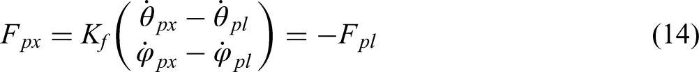
A fundamental model for the resistive force for the platform-pen motion is difficult to formulate but fortunately a simple empirical model is sufficient as it is just a mechanism for introducing some energy dissipation into the system and its relative magnitude can be controlled by changing the mass of the pendulum bobs. To progress the analysis a model for the resistive force is proposed of the form,

$$F_{px}=K_f\left(\begin{array}{c}{\dot{\theta }}_{px}-{\dot{\theta }}_{pl}\\ {\dot{\phi }}_{px}-{\dot{\phi }}_{pl}\end{array}\right)=-F_{pl}$$

(14)

where K_f is an adjustable constant. This is a similar approach used for other pendulum models,.^1,4 The system of equations for the rotary harmonograph motion is,

$${\ddot{\theta }}_{px}-{\displaystyle \frac{(B+L_{px}\sin {\theta }_{px})}{L_{px}}\cos {\theta }_{px}{\dot{\phi }}_{px}^2+{\displaystyle \frac{g}{L_{px}}\sin {\theta }_{px}+{\kappa }_{px,\theta }\cos {\theta }_{px}({\dot{\theta }}_{px}-{\dot{\theta }}_{pl})=0}}$$

$${\ddot{\phi }}_{px}+\left({\displaystyle \frac{2L_{px}}{B+L_{px}\sin {\theta }_{px}}}\right)\cos {\theta }_{px}{\dot{\theta }}_{px}{\dot{\phi }}_{px}+{\kappa }_{px,\phi }\sin {\theta }_{px}({\dot{\phi }}_{px}-{\dot{\phi }}_{pl})=0$$

$${\ddot{\theta }}_{pl}-{\displaystyle \frac{(B+L_{pl}\sin {\theta }_{pl})}{L_{pl}}\cos {\theta }_{pl}{\dot{\phi }}_{pl}^2+{\displaystyle \frac{g}{L_{pl}}\sin {\theta }_{pl}-{\kappa }_{pl,\theta }\cos {\theta }_{pl}({\dot{\theta }}_{pl}-{\dot{\theta }}_{pe})=0}}$$

$${\ddot{\phi }}_{pl}+\left({\displaystyle \frac{2L_{pl}}{B+L_{pl}\sin {\theta }_{pl}}}\right)\cos {\theta }_{pl}{\dot{\theta }}_{pl}{\dot{\phi }}_{pl}-{\kappa }_{pl,\phi }\sin {\theta }_{pl}({\dot{\phi }}_{pl}-{\dot{\phi }}_{pe})=0$$

$${\kappa }_{px}={\displaystyle \frac{K_f{L}_{px,2}}{m}\left(\begin{array}{c}{L}_{px}^{-2}\\ {(B+L_{px}\sin {\theta }_{px})}^{-2}\end{array}\right)}$$

$${\kappa }_{pl}={\displaystyle \frac{K_f{L}_{pl,2}}{m}\left(\begin{array}{c}{L}_{pl}^{-2}\\ {(B+L_{pl}\sin {\theta }_{pl})}^{-2}\end{array}\right)}$$

(15)

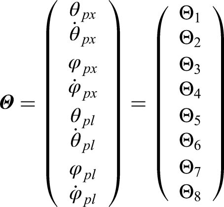
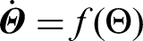
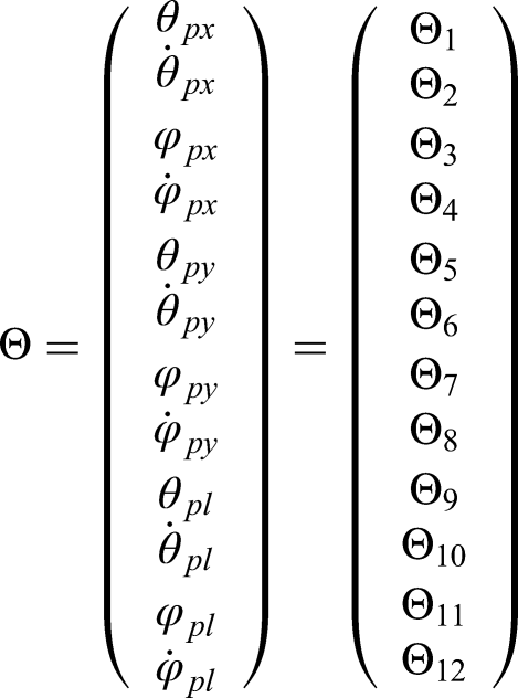
This system is solved using an ODE numerical solver once it is converted to a first order system,

$$\dot{\mathbf{\Theta }}=f(\mathrm{\Theta })$$

Where

$$\mathbf{\Theta }=\left(\begin{array}{c}\begin{array}{c}\begin{array}{c}{\theta }_{px}\\ {\dot{\theta }}_{px}\end{array}\\ \begin{array}{c}{\phi }_{px}\\ {\dot{\phi }}_{px}\end{array}\end{array}\\ \begin{array}{c}\begin{array}{c}{\theta }_{pl}\\ {\dot{\theta }}_{pl}\end{array}\\ \begin{array}{c}{\phi }_{pl}\\ {\dot{\phi }}_{pl}\end{array}\end{array}\end{array}\right)=\left(\begin{array}{c}\begin{array}{c}\begin{array}{c}{\mathrm{\Theta }}_1\\ {\mathrm{\Theta }}_2\end{array}\\ \begin{array}{c}{\mathrm{\Theta }}_3\\ {\mathrm{\Theta }}_4\end{array}\end{array}\\ \begin{array}{c}\begin{array}{c}{\mathrm{\Theta }}_5\\ {\mathrm{\Theta }}_6\end{array}\\ \begin{array}{c}{\mathrm{\Theta }}_7\\ {\mathrm{\Theta }}_8\end{array}\end{array}\end{array}\right)$$

$$f(\mathbf{\Theta })=\left(\begin{array}{c}{\mathrm{\Theta }}_2\\ \left({\displaystyle \frac{B+L_{px}\sin {\mathrm{\Theta }}_1}{L_{px}}}\right)\cos {\mathrm{\Theta }}_1{\mathrm{\Theta }}_4^2-{\displaystyle \frac{g}{L_{px}}\sin {\mathrm{\Theta }}_1-{\kappa }_{px,\theta }\cos {\mathrm{\Theta }}_1({\mathrm{\Theta }}_2-{\mathrm{\Theta }}_6)}\\ {\mathrm{\Theta }}_4\\ -\left({\displaystyle \frac{2L_{px}}{B+L_{px}\sin {\mathrm{\Theta }}_1}}\right)\cos {\mathrm{\Theta }}_1{\mathrm{\Theta }}_2{\mathrm{\Theta }}_4-{\kappa }_{px,\phi }\sin {\mathrm{\Theta }}_1({\mathrm{\Theta }}_4-{\mathrm{\Theta }}_8)\\ {\mathrm{\Theta }}_6\\ \left({\displaystyle \frac{B+L_{pl}\sin {\mathrm{\Theta }}_5}{L_{pl}}}\right)\cos {\mathrm{\Theta }}_5{\mathrm{\Theta }}_8^2-{\displaystyle \frac{g}{L_{pl}}\sin {\mathrm{\Theta }}_5-{\kappa }_{pl,\theta }\cos {\mathrm{\Theta }}_5({\mathrm{\Theta }}_6-{\mathrm{\Theta }}_2)}\\ {\mathrm{\Theta }}_8\\ -\left({\displaystyle \frac{2L_{pl}}{B+L_{pl}\sin {\mathrm{\Theta }}_5}}\right)\cos {\mathrm{\Theta }}_5{\mathrm{\Theta }}_6{\mathrm{\Theta }}_8-{\kappa }_{pl,\phi }\sin {\mathrm{\Theta }}_5({\mathrm{\Theta }}_8-{\mathrm{\Theta }}_4)\end{array}\right)$$

(16)

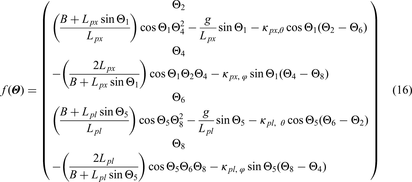
The system of differential equations, (16) is solved in MATLAB using the ode45 function. This is a variable step ODE solver, that uses 4^th and 5^th order Runge-Kutta methods. The system of differential equations is not stiff and does not represent a challenge to produce a numercal solution using the ode45 function.

2-pendulum kinematics

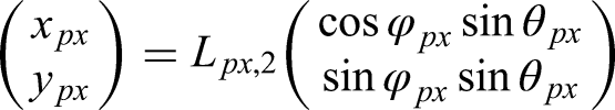
The relationship of the pen and platform dynamics, such as the location of the pen and location of the centre of the platform as well as the velocity of the pen and platform must be related to the conical pendulum dynamics. The kinematic relations for the pen and platform must be determined. From Figure 2 the pen location and platform centre location are,

$$\left(\begin{array}{c}{x}_{px}\\ y_{px}\end{array}\right)=L_{px,2}\left(\begin{array}{c}\cos {\phi }_{px}\sin {\theta }_{px}\\ \sin {\phi }_{px}\sin {\theta }_{px}\end{array}\right)$$

$$\left(\begin{array}{c}{x}_{pl}\\ y_{pl}\end{array}\right)=L_{pl,2}\left(\begin{array}{c}\cos {\phi }_{pl}\sin {\theta }_{pl}\\ \sin {\phi }_{pl}\sin {\theta }_{pl}\end{array}\right)$$

(17)

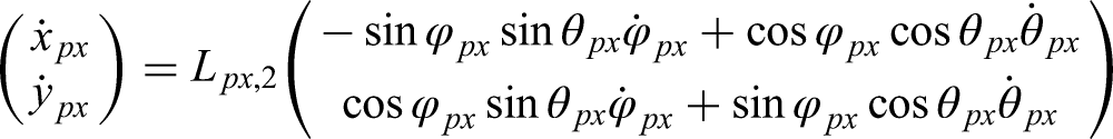
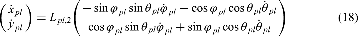
The velocity of the pen and platform in the x and y direction can be calculated by differentiating (17) with respect to time,

$$\left(\begin{array}{c}{\dot{x}}_{px}\\ {\dot{y}}_{px}\end{array}\right)=L_{px,2}\left(\begin{array}{c}-\sin {\phi }_{px}\sin {\theta }_{px}{\dot{\phi }}_{px}+\cos {\phi }_{px}\cos {\theta }_{px}{\dot{\theta }}_{px}\\ \cos {\phi }_{px}\sin {\theta }_{px}{\dot{\phi }}_{px}+\sin {\phi }_{px}\cos {\theta }_{px}{\dot{\theta }}_{px}\end{array}\right)$$

$$\left(\begin{array}{c}{\dot{x}}_{pl}\\ {\dot{y}}_{pl}\end{array}\right)=L_{pl,2}\left(\begin{array}{c}-\sin {\phi }_{pl}\sin {\theta }_{pl}{\dot{\phi }}_{pl}+\cos {\phi }_{pl}\cos {\theta }_{pl}{\dot{\theta }}_{pl}\\ \cos {\phi }_{pl}\sin {\theta }_{pl}{\dot{\phi }}_{pl}+\sin {\phi }_{pl}\cos {\theta }_{pl}{\dot{\theta }}_{pl}\end{array}\right)$$

(18)

2-pendulum harmonograph initial conditions

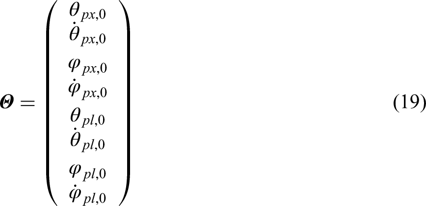
The final component of the model is some way to initiate the harmonograph. The conical pendulums require initial conditions of the form,

$$\mathbf{\Theta }=\left(\begin{array}{c}\begin{array}{c}\begin{array}{c}{\theta }_{px,0}\\ {\dot{\theta }}_{px,0}\end{array}\\ \begin{array}{c}{\phi }_{px,0}\\ {\dot{\phi }}_{px,0}\end{array}\end{array}\\ \begin{array}{c}\begin{array}{c}{\theta }_{pl,0}\\ {\dot{\theta }}_{pl,0}\end{array}\\ \begin{array}{c}{\phi }_{pl,0}\\ {\dot{\phi }}_{pl,0}\end{array}\end{array}\end{array}\right)$$

(19)

This is an 8-dimensional space, and it is impractical to specify initial pendulum conditions that are likely to produce an interesting geometric design. The way forward for specifying the harmonograph initial conditions is to mimic the way a real harmonograph is initiated. For a real harmonograph the device is initiated by the pen and platform being moved by the user until a design that looks like it might be interesting is evolving. At this point the user releases the platform, lowers the pen on to the platform, and the process is driven by the pendulum motion.

The basis of the initial condition prescription is specified to be an ellipse. The parametric equations for an ellipse can be stated as,

$$\left(\begin{array}{c}x\\ y\end{array}\right)=\left(\begin{array}{c}{a}_{pen}\cos c_{pen}{t}_{rel}\\ b_{pen}\sin c_{pen}{t}_{rel}\end{array}\right)$$

(20)

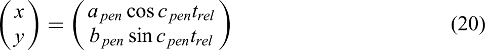
Where t_rel is the time, the pen is released, and the generation of the drawing begins. This is not quite general enough as the ellipse given by (20) is aligned with the x axis and y axis. It can be generalised to an ellipse centred on the origin with any orientation by applying a rotation matrix to (20).

$$\left(\begin{array}{c}{x}_{px,0}\\ y_{px,0}\end{array}\right)=\left(\begin{array}{c}{a}_{pen}\cos c_{pen}{t}_{rel}\cos \psi +b_{pen}\sin c_{pen}{t}_{rel}\sin \psi \\ -a_{pen}\cos c_{pen}{t}_{rel}\sin \psi +b_{pen}\sin c_{pen}{t}_{rel}\cos \psi \end{array}\right)$$

(21)

Where a_pen, b_pen, c_pen, and ψ are constants determining the ellipse used for the initial pendulum conditions, and t_rel is the time of release of the pen. The velocity of the pen can be determined by differentiating (21) with respect to time.

$$\left(\begin{array}{c}{\dot{x}}_{px,0}\\ {\dot{y}}_{px,0}\end{array}\right)=\left(\begin{array}{c}-a_{pen}{c}_{pen}\sin c_{pen}{t}_{rel}\cos \psi +b_{pen}{c}_{pen}\cos c_{pen}{t}_{rel}\sin \psi \\ a_{pen}{c}_{pen}\sin c_{pen}{t}_{rel}\sin \psi +b_{pen}{c}_{pen}\cos c_{pen}{t}_{rel}\cos \psi \end{array}\right)$$

(22)

The analysis for the initial condition for the platform is similar.

The kinematic conditions are used to relate the pen and platform location and trajectory to the pendulum conditions once the simulation is initiated. For the initial conditions for the pendulums the kinematic conditions are applied in reverse. The analysis will be presented for the pen alone as the analysis for the platform initial location and trajectory is similar. Taking $\left(\begin{array}{c}{x}_{px,0}\\ y_{px,0}\end{array}\right)$ and $\left(\begin{array}{c}{\dot{x}}_{px,0}\\ {\dot{y}}_{px,0}\end{array}\right)$ as given by (21, 22), and solving for θ_pe,0 and φ_pe,0.

$${\phi }_{px,0}={\tan }^{-1}\left({\displaystyle \frac{y_{px,0}}{x_{px,0}}}\right)$$

$${\theta }_{px,0}={\sin }^{-1}\left({\displaystyle \frac{x_{px,0}}{\cos {\phi }_{px,0}}}\right)$$

(23)

When taking the inverse tangent care must be taken as to which quadrant the initial condition is in, based on the signs of x_pe,0 and y_pe,0. The pens initial trajectory can be used to determine the angular velocities for the conical pendulum attached to the pen. The initial angular velocities of the conical pendulum are determined by solving the linear system,

$$\left(\begin{array}{c}{\dot{x}}_{px,0}\\ {\dot{y}}_{px,0}\end{array}\right)=L_{px,2}\left(\begin{array}{cc}-\sin {\phi }_{px,0}\sin {\theta }_{px,0}& \cos {\phi }_{px,0}\cos {\theta }_{px,0}\\ \cos {\phi }_{px,0}\sin {\theta }_{px,0}& \sin {\phi }_{px,0}\cos {\theta }_{px,0}\end{array}\right)\left(\begin{array}{c}{\dot{\phi }}_{px,0}\\ {\dot{\theta }}_{px,0}\end{array}\right)$$

(24)

The mathematical model for a 2-pendulum rotary harmonograph is complete and it is possible to simulate a 2-pendulum rotary harmonograph.

Simulations of a 2-pendulum harmonograph

There are many parameters that define the rotary harmonograph, there are too many to comprehensively explore parameter space. Fortunately, there are some physical constraints that define narrow ranges for some parameters. For all simulations unless stated otherwise have the following values: the mass of the pendulum, m = 1 kg, the parameter L_px,2 = 0.5 m and, L_pl,2 = 0.8L_px,2. The length of the pendulums is specified indirectly by prescribing the natural frequencies of the pendulums.

$$L_{px}={\displaystyle \frac{g}{{\omega }_x^2},L_{pl}={\displaystyle \frac{g}{{\omega }_{pl}^2}}}$$

(25)

In a real rotary harmonograph the length of the pendulums is restricted by the physical space available. For a mathematical model this is not an issue. In general, for a harmonograph, the pen resistive force, F_pen is small compared to the weight of the pendulum bobs. In the simulations presented below K_f is treated as a free parameter.

The geometric designs produced by a harmonograph depend on the natural frequencies of the pendulums, initial conditions of the pendulums defining the location and speed of the pen and platform and the balance between the pendulum weights and frictional force.

The first simulation considered, Test 1 is two pendulums with natural frequencies, ω_px = ω_pl = 2 rad/s and the initial conditions of the pen and platform have an initially circulating motion defined by,

$$a_{pen}=b_{pen}=0.2,c_{pen}=1,t_{rel}=1s,{\psi }_{pen}={\displaystyle \frac{\pi }{4}}$$

$$a_{pl}=b_{pl}=0.2,c_{pl}=-1,t_{rel}=1s,{\psi }_{pl}={\displaystyle \frac{\pi }{4}}$$

(26)

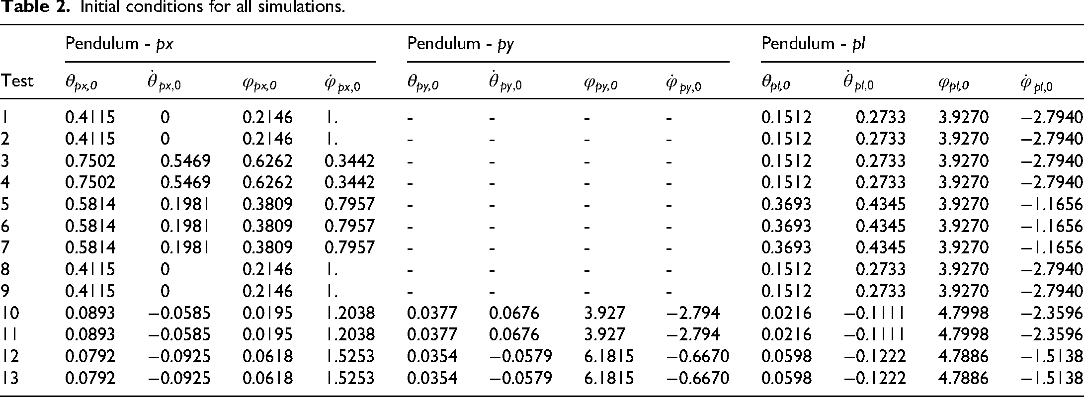
These parameters give a pen that has an initially circular motion with an anticlockwise sense of rotation and the platform has a clockwise sense of rotation. The simulation conditions for all tests are summarised in Table 1. The initial conditions for the pendulums for all simulations are summarised in Table 2.

Table 1.

Summary of harmonograph simulations. ^*

Test	ωpx	ωpy	ωpl	apen, bpen, cpen	apl, bpl, cpl	Kf	tsim / s
1	2	-	2	0.2, 0.2, 1	0.2, 0.2, −1	0	300
2	2	-	2	0.2, 0.2, 1	0.2, 0.2, −1	0.01	300
3	2	-	2	0.1, 0.4, 1	0.2, 0.2, −1	0	300
4	2.01	-	1.99	0.1, 0.4, 1	0.2, 0.2, −1	0	300
5	2.99	-	3.01	0.2, 0.3, 1	0.2, 0.3, −1	0	300
6	2.99	-	3.01	0.2, 0.3, 1	0.2, 0.3, −1	0.001	300
7	2.99	-	3.01	0.2, 0.3, 1	0.2, 0.3, −1	0.01	300
8	1	-	3	0.2, 0.2, 1	0.2, 0.2, −1	0.001	600
9	3	-	3	0.2, 0.2, 1	0.2, 0.2, −1	0.001	300
10	3.99	3.99	4.01	0.07, 0.03, 1	0.05, 0.05, −1	0	200
11	3.99	3.99	4.01	0.07, 0.03, 1	0.05, 0.05, −1	0.001	200
12	3	1	2	0.09, 0.01,1	0.05, 0.05, −0.5	0	300
13	2.99	1.01	1.99	0.09, 0.01,1	0.05, 0.05, −0.5	0	300

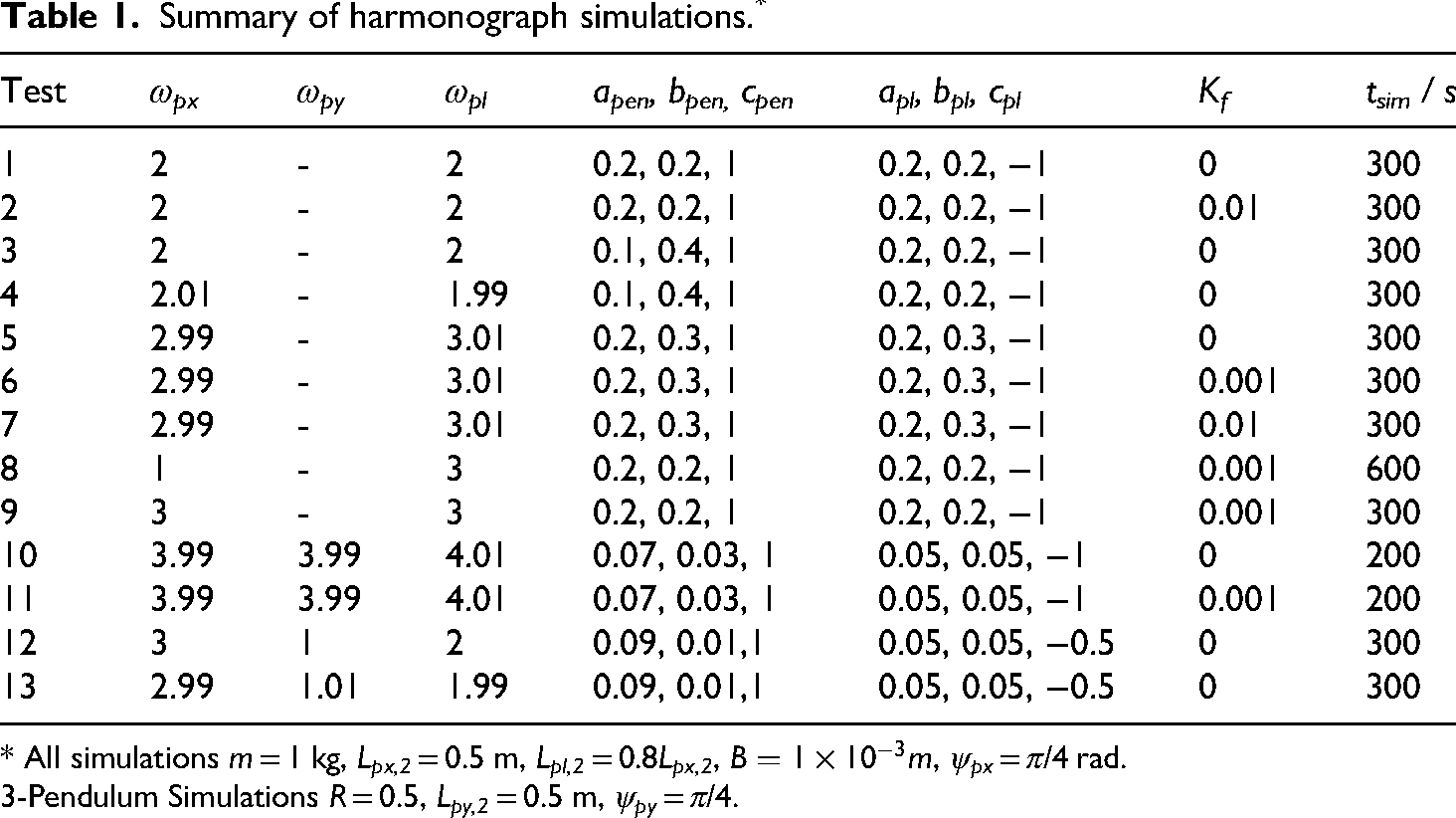
* All simulations m = 1 kg, L_px,2 = 0.5 m, L_pl,2 = 0.8L_px,2, $B=1\times {10}^{-3}m$ , ψ_px = π/4 rad.

3-Pendulum Simulations R = 0.5, L_py,2 = 0.5 m, ψ_py = π/4.

Table 2.

Initial conditions for all simulations.

Test	Pendulum - px				Pendulum - py				Pendulum - pl
	θpx,0	${\dot{\theta }}_{px,0}$	φpx,0	${\dot{\phi }}_{px,0}$	θpy,0	${\dot{\theta }}_{py,0}$	φpy,0	${\dot{\phi }}_{py,0}$	θpl,0	${\dot{\theta }}_{pl,0}$	φpl,0	${\dot{\phi }}_{pl,0}$
1	0.4115	0	0.2146	1.	-	-	-	-	0.1512	0.2733	3.9270	−2.7940
2	0.4115	0	0.2146	1.	-	-	-	-	0.1512	0.2733	3.9270	−2.7940
3	0.7502	0.5469	0.6262	0.3442	-	-	-	-	0.1512	0.2733	3.9270	−2.7940
4	0.7502	0.5469	0.6262	0.3442	-	-	-	-	0.1512	0.2733	3.9270	−2.7940
5	0.5814	0.1981	0.3809	0.7957	-	-	-	-	0.3693	0.4345	3.9270	−1.1656
6	0.5814	0.1981	0.3809	0.7957	-	-	-	-	0.3693	0.4345	3.9270	−1.1656
7	0.5814	0.1981	0.3809	0.7957	-	-	-	-	0.3693	0.4345	3.9270	−1.1656
8	0.4115	0	0.2146	1.	-	-	-	-	0.1512	0.2733	3.9270	−2.7940
9	0.4115	0	0.2146	1.	-	-	-	-	0.1512	0.2733	3.9270	−2.7940
10	0.0893	−0.0585	0.0195	1.2038	0.0377	0.0676	3.927	−2.794	0.0216	−0.1111	4.7998	−2.3596
11	0.0893	−0.0585	0.0195	1.2038	0.0377	0.0676	3.927	−2.794	0.0216	−0.1111	4.7998	−2.3596
12	0.0792	−0.0925	0.0618	1.5253	0.0354	−0.0579	6.1815	−0.6670	0.0598	−0.1222	4.7886	−1.5138
13	0.0792	−0.0925	0.0618	1.5253	0.0354	−0.0579	6.1815	−0.6670	0.0598	−0.1222	4.7886	−1.5138

For Test 1 the simulation run-time is 300 s. The geometric design produced is shown in Figure 3(a), and the design produced resembles a flower with six petals. It is difficult to relate the design back to the initial conditions and the natural frequencies of the system. Test 2 has the same specification as Test 1 except, it includes frictional losses associated with the motion of the pen on the platform, K_f = 0.01 Ns/rad. For Test 2 the simulated pen trajectory relative to the centre of the platform is shown in Figure 3(b). The initial transient for Test 2, as expected is similar to Test 1, but very quickly the trajectory spirals into the origin, a stable equilibrium point. Test 1 and Test 2 demonstrate that the geometric design produced by a harmonograph is sensitive to the frictional loss coefficient. This will be investigated further below as Figure 3(b) suggests a value of K_f = 0.01 Ns/rad for m = 1 kg represents a large frictional force.

Figure 3.

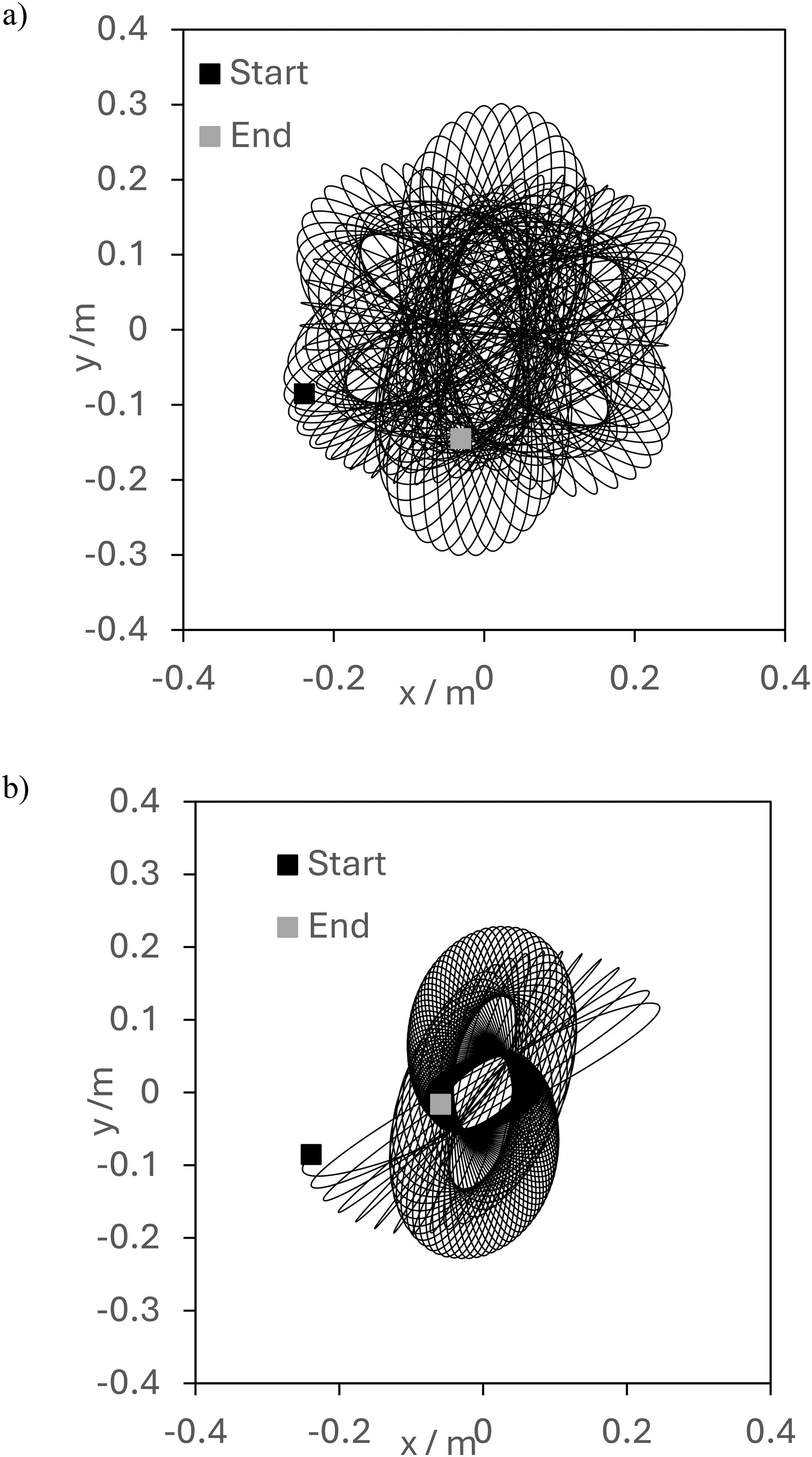
Geometric design produced for (a) Test 1, (ω_px, ω_pl) = (2, 2), K_f = 0 and (b) Test 2, (ω_px, ω_pl) = (2, 2), K_f = 0.01 Ns/rad.

For the third simulation considered, the initial condition for the pen is changed to have an elliptical trajectory,

$$a_{pen}=0.1,b_{pen}=0.4,c_{pen}=1,t_{rel}=1s,{\psi }_{pen}={\displaystyle \frac{\pi }{4}}$$

$$a_{pl}=b_{pl}=0.2,c_{pl}=-1,t_{rel}=1s,{\psi }_{pl}={\displaystyle \frac{\pi }{4}}$$

(27)

The natural frequencies are the same as Test 1 and Test 2, (ω_px, ω_pl) = (2, 2). Similar to Test 1 and Test 2 the simulation time is 300 s. The geometric design generated for the Test 3 conditions is shown in Figure 4(a). The elliptical initial condition produces a much different geometric design from Test 1. For Test 3, after the initial transient the design resembles a series of four-sided shapes with a quasi-symmetry of π/2 that would be expected for the natural frequencies prescribed. If the simulation for Test 3 were continued to t_sim = 600 s the design evolves into a cross like shape.

Figure 4.

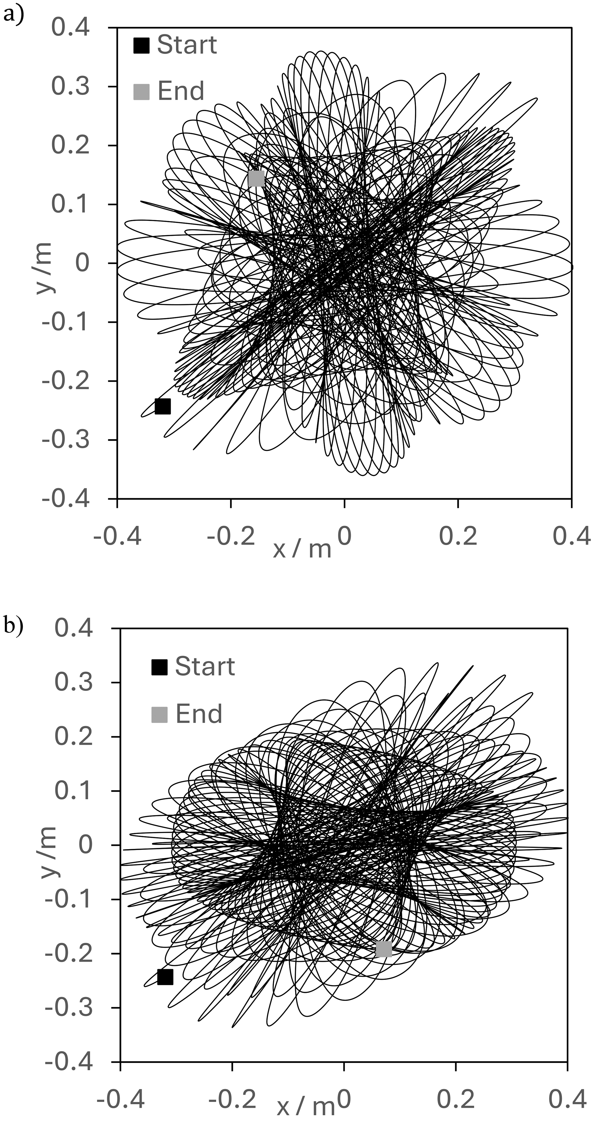
Geometric design produced for elliptical initial conditions, (a) Test 3, (ω_px, ω_pl) = (2, 2), and (b) Test 4, (ω_px, ω_pl) = (2.01, 1.99).

Often it is interesting to simulate a harmonograph with natural frequencies perturbed from integer values. Test 4 is similar to Test 3 except, (ω_px, ω_pl) = (2.01, 1.99) rad/s, a relative change of 0.5%. The geometric design produced for the Test 4 conditions is shown in Figure 4(b). The geometric design beyond the initial transient has a four-sided structure but there the similarity with Test 3 ends. If the simulation time is doubled to t_sim = 600 s there is no cross-like structure and the design asymptotes to the origin. The geometric design produced for the Test 4 conditions is very different from the Test 3 design when the small changes in natural frequency are factored into the analysis. This has a practical impact on the design of a physical harmonograph as there are always errors in the prescribed natural frequencies of the pendulums.

Test 1 and Test 2 show that the geometric design produced changes radically when the frictional loss is introduced to account for the movement of the pen on the moving platform. The next set of simulations consider the sensitivity of the geometric design produced for different values of K_f. Test 5, Test 6 and Test 7 have the same initial conditions and natural frequencies,

$$a_{pen}=0.1,b_{pen}=0.4,c_{pen}=1,t_{rel}=1s,{\psi }_{pen}={\displaystyle \frac{\pi }{4}rad}$$

$$a_{pl}=b_{pl}=0.2,c_{pl}=-1,t_{rel}=1s,{\psi }_{pl}={\displaystyle \frac{\pi }{4}rad}$$

$$({\omega }_{px},{\omega }_{pl})=(2.99,3.01){\displaystyle \frac{rad}{s}}$$

(28)

For each of the three tests the simulation time is the same, t_sim = 300 s. The three tests have different values for the friction coefficient, Test 5, K_f = 0, Test 6, K_f = 0.001 Ns/rad and Test 7, K_f = 0.01 Ns/rad. The simulated harmonograph patterns for each test are shown in Figure 5.

Figure 5.

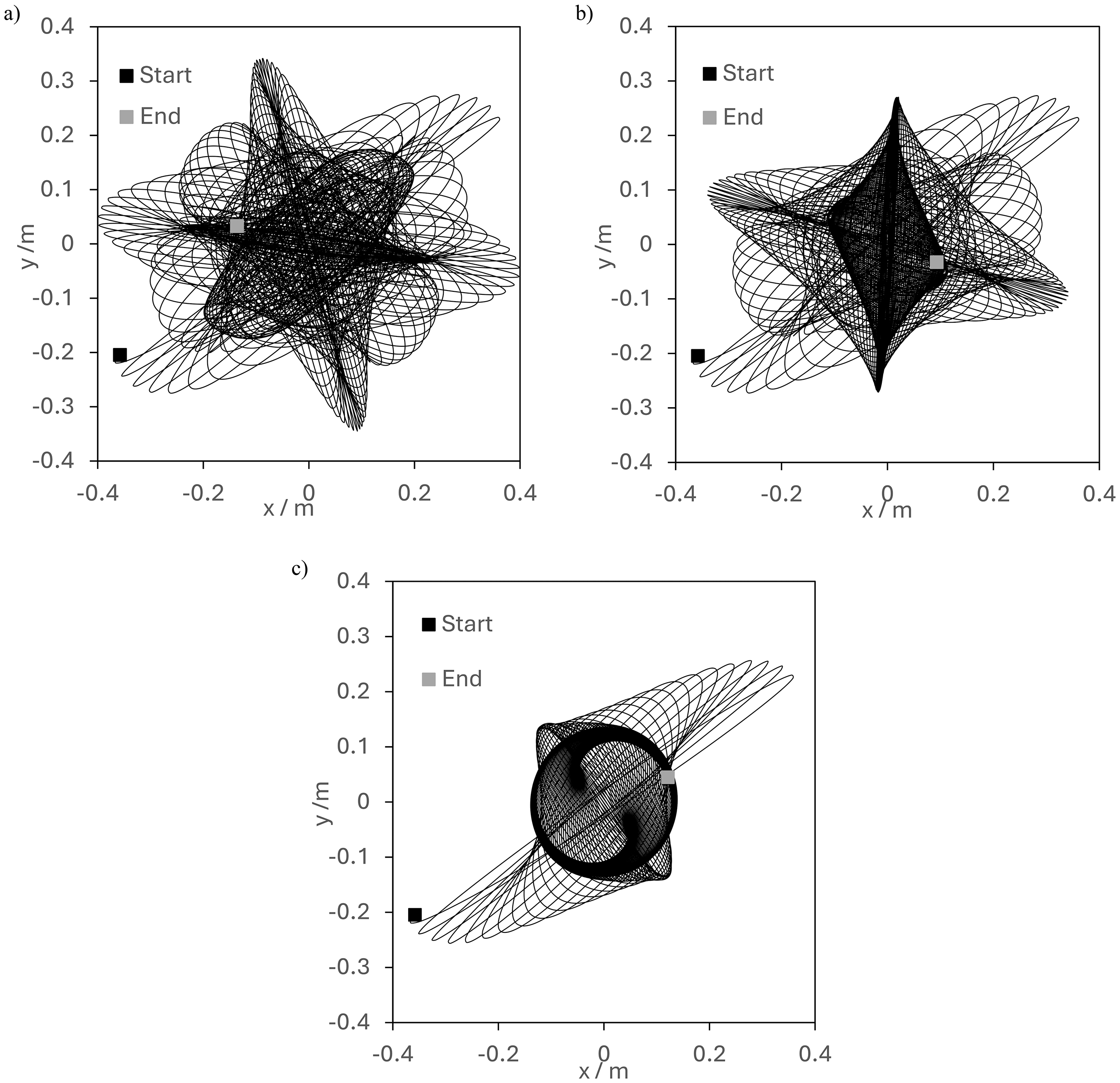
Geometric design produced for (a) Test 5, (ω_px,ω_pl) = (2.99, 3.01), K_f = 0, (b) Test 6, K_f = 0.001 Ns/rad, and (c) Test 7, K_f = 0.01 Ns/rad.

The geometric pattern produced for Test 5 is shown in Figure 5(a), it is an interesting design but cannot easily be related to the initial conditions and natural frequencies of the system. The geometric pattern produced for Test 6 is shown in Figure 5(b). For this simulation the friction coefficient is K_f = 0.001 Ns/rad, and the pattern produced is very different from Test 5 with no frictional losses, see Figure 5(a). For the simulation time of t_sim = 300 s Figure 5(b) suggests that the pen trajectory asymptotes to a line close to x = 0, continuing the simulation to 600 s shows that the pen trajectory converges on the origin as expected.

The final simulation in this series, Test 7, with a much larger friction coefficient, K_f = 0.01 Ns/rad is shown in Figure 5(c). The geometric pattern generated for the first 300 s of simulation time shows the initial transient asymptotes to a circular trajectory. Continuing the simulation for another 300 s, t_sim = 600 s, shows the circular trajectory decays towards the origin.

One conclusion that can be drawn from Figure 5 is that the geometric pattern produced by the harmonograph is sensitive to the friction force imposed on the system.

The last two simulations for the 2-pendulum rotary harmonograph, Test 8 and Test 9, illustrate how the dynamics of a harmonograph depend on how the frictional loss and natural frequencies interact. Test 8 and Test 9 are defined to both have circular initial conditions, see Table 1, both tests have a frictional loss coefficient, K_f = 0.001 Ns/rad. For Test 8 the natural frequencies are,

$$({\omega }_{px},{\omega }_{pl})=(1,3){\displaystyle \frac{rad}{s}}$$

(29)

and a simulation time of t_sim = 600 s. For Test 9, t_sim = 300 s and the natural frequencies are,

$$({\omega }_{px},{\omega }_{pl})=(3,3){\displaystyle \frac{rad}{s}}$$

(30)

The simulated pen trajectories are shown in Figure 6(a) and (b). The geometric pattern generated for the Test 8 specification is shown in Figure 6(a) and is rotationally symmetric and converges to an annulus. For longer simulation times the outer radius of the annulus converges to the origin. For Test 9, the geometric design is shown in Figure 6(b) and is more interesting than Figure 6(a). In Figure 6(b), Test 9 the pen trajectory asymptotes to an ellipse, and given that the simulation time is half that of Test 8 the rate of convergence to the origin is much larger than for Test 8.

Figure 6.

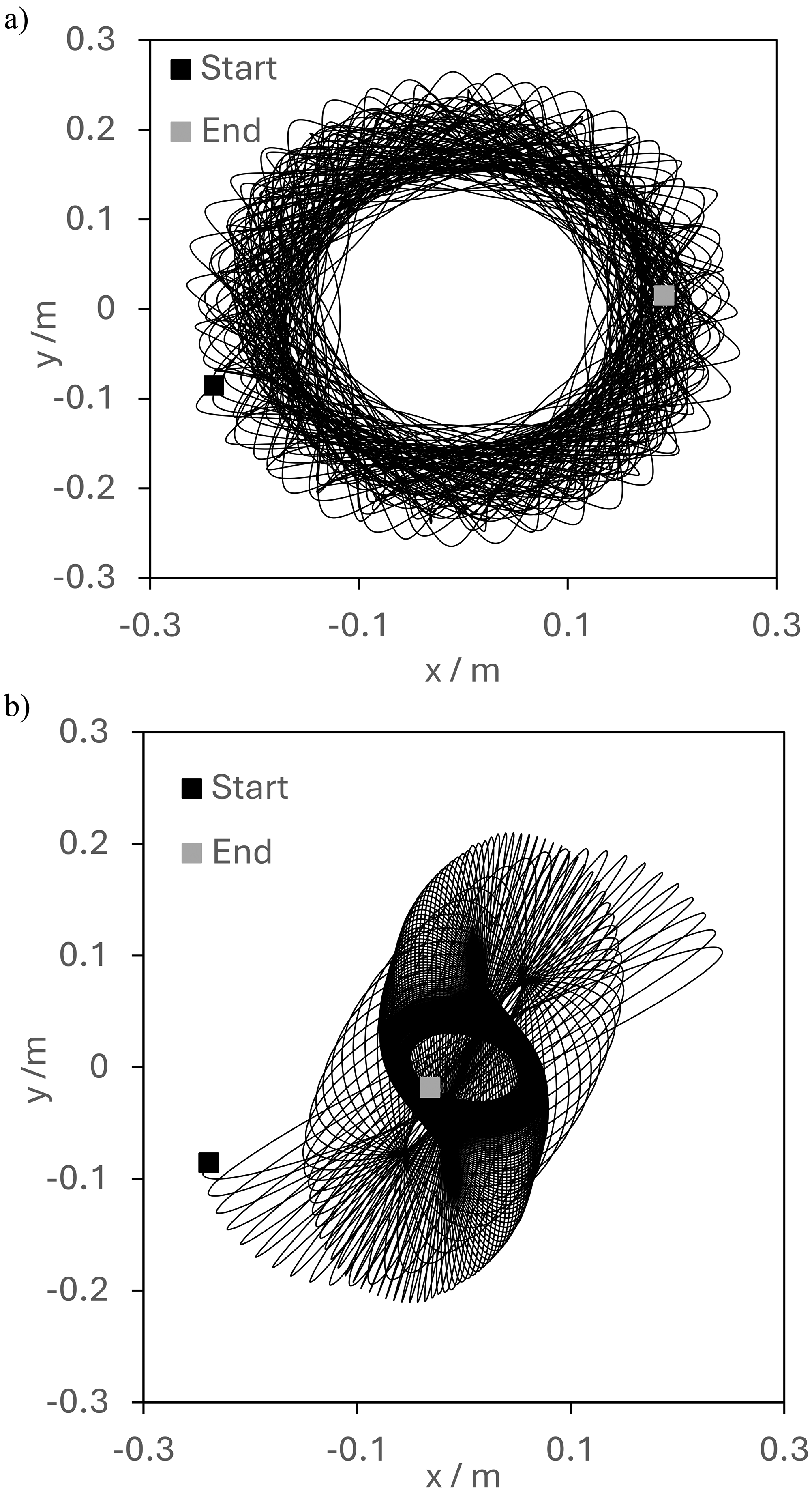
Geometric design produced for (a) Test 8, K_f = 0.001 Ns/rad, (ω_px, ω_pl) = (1, 3), and (b) Test 9, (ω_px, ω_pl) = (3, 3).

This behaviour can be explained by looking at the ratio of the two parameters, κ_px,θ and κ_pl,θ. These two parameters depend on the frictional loss and the length of the pendulums making them implicitly dependant on the natural frequencies of the pendulums such that for Test 8,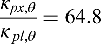

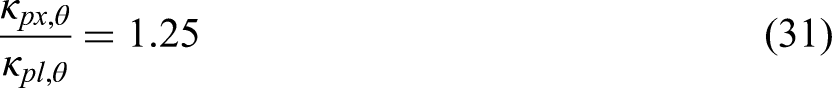
$${\displaystyle \frac{{\kappa }_{px,\theta }}{{\kappa }_{pl,\theta }}=64.8}$$

and for Test 9 the ratio is,

$${\displaystyle \frac{{\kappa }_{px,\theta }}{{\kappa }_{pl,\theta }}=1.25}$$

(31)

This means that for Test 8 the pendulum driving the motion of the pen relatively quickly converges to a near stationary pendulum, the equilibrium state. The platform motion driven by a conical pendulum continues with its circular motion giving the geometric pattern shown in Figure 6(a). In Test 9 the frictional loss is more evenly balanced giving an asymptotic elliptical trajectory for the pen relative to the platform that converges to the origin in a much shorter time interval.

3-pendulum rotary harmonograph

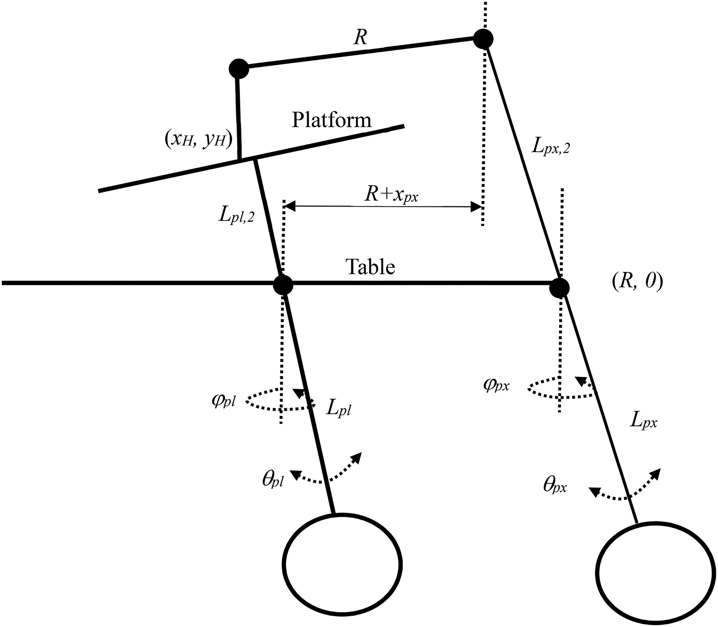
A schematic of a 3-pendulum rotary harmonograph is shown in Figure 7. The gimbles for the conical pendulums are located at (R, 0) and (0, R) where R is the length of a connecting rod between the pendulum and the pen.

Figure 7.

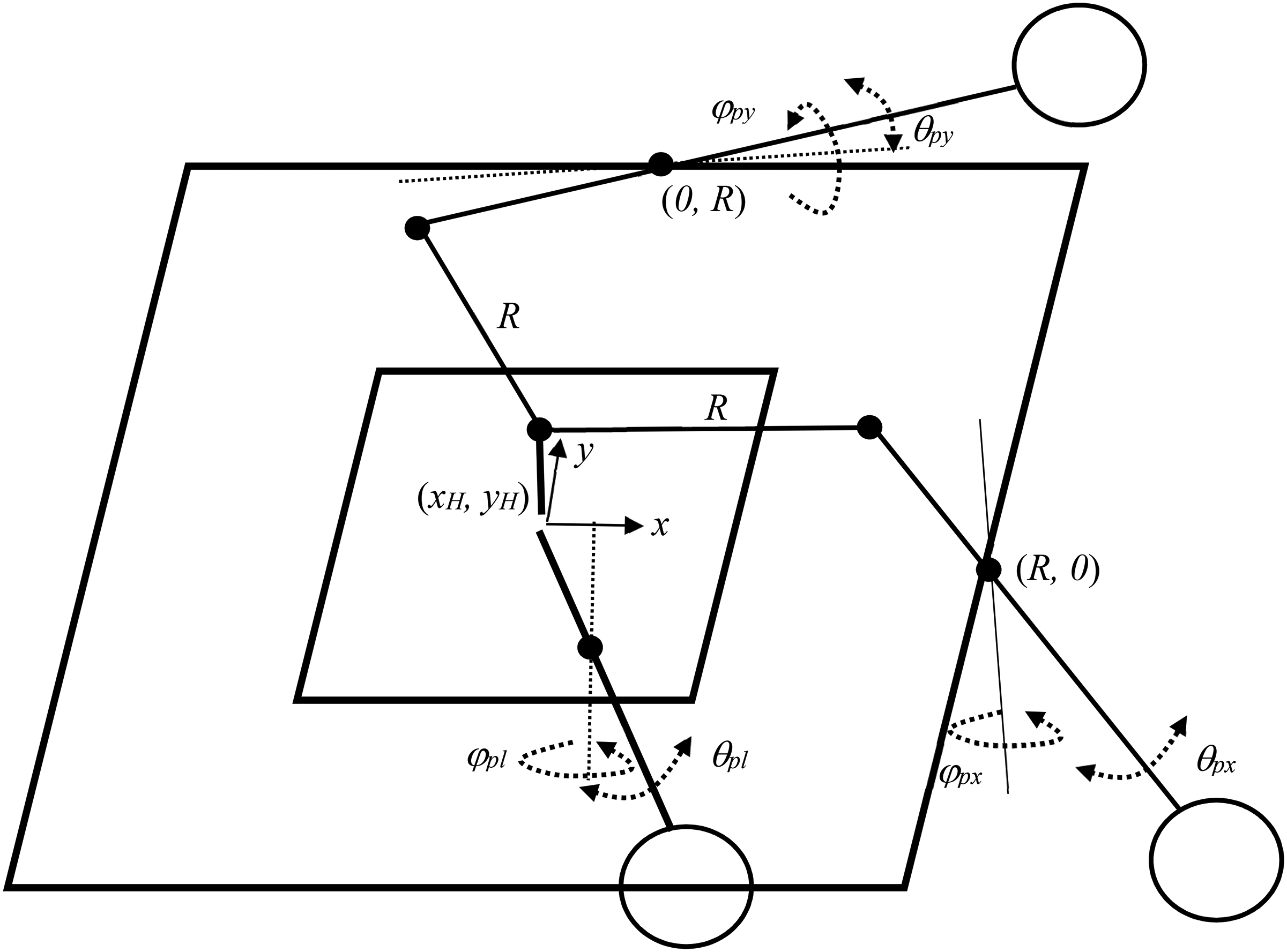
Schematic diagram of a 3-pendulum rotary harmonograph.

3-pendulum rotary harmonograph model

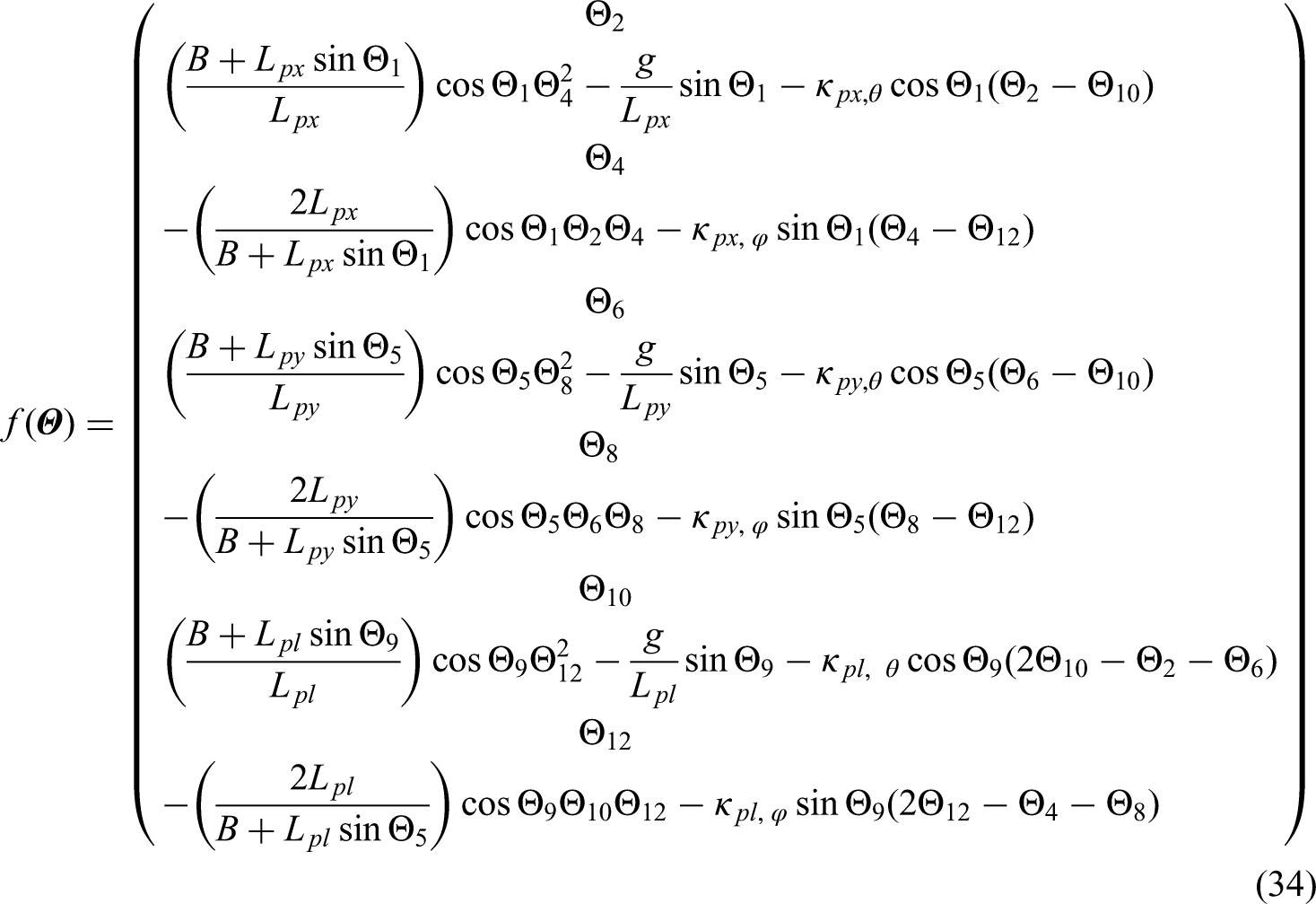
The basis of the 3-pendulum rotary harmonograph model is three conical pendulums that move independently of each other except frictional loss due to the motion of the pen and the platform. The basis is very similar to the 2-pendulum rotary harmonograph except there are two pendulums controlling the movement of the pen. The basis of the 3-pendulum rotary harmonograph model is,

$${\ddot{\theta }}_{px}-{\displaystyle \frac{(B+L_{px}\sin {\theta }_{px})}{L_{px}}\cos {\theta }_{px}{\dot{\phi }}_{px}^2+{\displaystyle \frac{g}{L_{px}}\sin {\theta }_{px}+{\kappa }_{px,\theta }\cos {\theta }_{px}({\dot{\theta }}_{px}-{\dot{\theta }}_{pl})=0}}$$

$${\ddot{\phi }}_{px}+\left({\displaystyle \frac{2L_{px}}{B+L_{px}\sin {\theta }_{px}}}\right)\cos {\theta }_{px}{\dot{\theta }}_{px}{\dot{\phi }}_{px}+{\kappa }_{px,\phi }\sin {\theta }_{px}({\dot{\phi }}_{px}-{\dot{\phi }}_{pl})=0$$

$${\ddot{\theta }}_{py}-{\displaystyle \frac{(B+L_{py}\sin {\theta }_{py})}{L_{py}}\cos {\theta }_{py}{\dot{\phi }}_{py}^2+{\displaystyle \frac{g}{L_{py}}\sin {\theta }_{py}+{\kappa }_{py,\theta }\cos {\theta }_{py}({\dot{\theta }}_{py}-{\dot{\theta }}_{pl})=0}}$$

$${\ddot{\phi }}_{py}+\left({\displaystyle \frac{2L_{py}}{B+L_{py}\sin {\theta }_{py}}}\right)\cos {\theta }_{py}{\dot{\theta }}_{py}{\dot{\phi }}_{py}+{\kappa }_{py,\phi }\sin {\theta }_{py}({\dot{\phi }}_{py}-{\dot{\phi }}_{pl})=0$$

$${\ddot{\theta }}_{pl}-{\displaystyle \frac{(B+L_{pl}\sin {\theta }_{pl})}{L_{pl}}\cos {\theta }_{pl}{\dot{\phi }}_{pl}^2+{\displaystyle \frac{g}{L_{pl}}\sin {\theta }_{pl}+{\kappa }_{pl,\theta }\cos {\theta }_{pl}(2{\dot{\theta }}_{pl}-({\dot{\theta }}_{px}+{\dot{\theta }}_{py}))=0}}$$

$${\ddot{\phi }}_{pl}+\left({\displaystyle \frac{2L_{pl}}{B+L_{pl}\sin {\theta }_{pl}}}\right)\cos {\theta }_{pl}{\dot{\theta }}_{pl}{\dot{\phi }}_{pl}+{\kappa }_{pl,\phi }\sin {\theta }_{pl}(2{\dot{\phi }}_{pl}-({\dot{\phi }}_{px}+{\dot{\phi }}_{py}))=0$$

$${\kappa }_{px}={\displaystyle \frac{K_f{L}_{px,2}}{m}\left(\begin{array}{c}{L}_{px}^{-2}\\ {(B+L_{px}\sin {\theta }_{px})}^{-2}\end{array}\right)}$$

$${\kappa }_{py}={\displaystyle \frac{K_f{L}_{py,2}}{m}\left(\begin{array}{c}{L}_{py}^{-2}\\ {(B+L_{py}\sin {\theta }_{py})}^{-2}\end{array}\right)}$$

$${\kappa }_{pl}={\displaystyle \frac{K_f{L}_{pl,2}}{m}\left(\begin{array}{c}{L}_{pl}^{-2}\\ {(B+L_{pl}\sin {\theta }_{pl})}^{-2}\end{array}\right)}$$

(32)

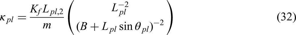
The only point of note is that the frictional loss term in the differential equations has been extended from the 2-pendulum rotary harmonograph model such that the condition,

$$F_{px}+F_{py}=-F_{pl}$$

(33)

is satisfied. The 3-pendulum harmonograph model is solved numerically by converting the system to a first order system of differential equations,

$$\dot{\mathbf{\Theta }}=f(\mathrm{\Theta })$$

where

$$\mathrm{\Theta }=\left(\begin{array}{c}\begin{array}{c}\begin{array}{c}{\theta }_{px}\\ {\dot{\theta }}_{px}\end{array}\\ \begin{array}{c}{\phi }_{px}\\ {\dot{\phi }}_{px}\end{array}\end{array}\\ \begin{array}{c}\begin{array}{c}{\theta }_{py}\\ {\dot{\theta }}_{py}\end{array}\\ \begin{array}{c}{\phi }_{py}\\ {\dot{\phi }}_{py}\end{array}\end{array}\\ \begin{array}{c}\begin{array}{c}{\theta }_{pl}\\ {\dot{\theta }}_{pl}\end{array}\\ \begin{array}{c}{\phi }_{pl}\\ {\dot{\phi }}_{pl}\end{array}\end{array}\end{array}\right)=\left(\begin{array}{c}\begin{array}{c}\begin{array}{c}{\mathrm{\Theta }}_1\\ {\mathrm{\Theta }}_2\end{array}\\ \begin{array}{c}{\mathrm{\Theta }}_3\\ {\mathrm{\Theta }}_4\end{array}\end{array}\\ \begin{array}{c}\begin{array}{c}{\mathrm{\Theta }}_5\\ {\mathrm{\Theta }}_6\end{array}\\ \begin{array}{c}{\mathrm{\Theta }}_7\\ {\mathrm{\Theta }}_8\end{array}\end{array}\\ \begin{array}{c}\begin{array}{c}{\mathrm{\Theta }}_9\\ {\mathrm{\Theta }}_{10}\end{array}\\ \begin{array}{c}{\mathrm{\Theta }}_{11}\\ {\mathrm{\Theta }}_{12}\end{array}\end{array}\end{array}\right)$$

$$f(\mathbf{\Theta })=\left(\begin{array}{c}{\mathrm{\Theta }}_2\\ \left({\displaystyle \frac{B+L_{px}\sin {\mathrm{\Theta }}_1}{L_{px}}}\right)\cos {\mathrm{\Theta }}_1{\mathrm{\Theta }}_4^2-{\displaystyle \frac{g}{L_{px}}\sin {\mathrm{\Theta }}_1-{\kappa }_{px,\theta }\cos {\mathrm{\Theta }}_1({\mathrm{\Theta }}_2-{\mathrm{\Theta }}_{10})}\\ {\mathrm{\Theta }}_4\\ -\left({\displaystyle \frac{2L_{px}}{B+L_{px}\sin {\mathrm{\Theta }}_1}}\right)\cos {\mathrm{\Theta }}_1{\mathrm{\Theta }}_2{\mathrm{\Theta }}_4-{\kappa }_{px,\phi }\sin {\mathrm{\Theta }}_1({\mathrm{\Theta }}_4-{\mathrm{\Theta }}_{12})\\ {\mathrm{\Theta }}_6\\ \left({\displaystyle \frac{B+L_{py}\sin {\mathrm{\Theta }}_5}{L_{py}}}\right)\cos {\mathrm{\Theta }}_5{\mathrm{\Theta }}_8^2-{\displaystyle \frac{g}{L_{py}}\sin {\mathrm{\Theta }}_5-{\kappa }_{py,\theta }\cos {\mathrm{\Theta }}_5({\mathrm{\Theta }}_6-{\mathrm{\Theta }}_{10})}\\ {\mathrm{\Theta }}_8\\ -\left({\displaystyle \frac{2L_{py}}{B+L_{py}\sin {\mathrm{\Theta }}_5}}\right)\cos {\mathrm{\Theta }}_5{\mathrm{\Theta }}_6{\mathrm{\Theta }}_8-{\kappa }_{py,\phi }\sin {\mathrm{\Theta }}_5({\mathrm{\Theta }}_8-{\mathrm{\Theta }}_{12})\\ {\mathrm{\Theta }}_{10}\\ \left({\displaystyle \frac{B+L_{pl}\sin {\mathrm{\Theta }}_9}{L_{pl}}}\right)\cos {\mathrm{\Theta }}_9{\mathrm{\Theta }}_{12}^2-{\displaystyle \frac{g}{L_{pl}}\sin {\mathrm{\Theta }}_9-{\kappa }_{pl,\theta }\cos {\mathrm{\Theta }}_9(2{\mathrm{\Theta }}_{10}-{\mathrm{\Theta }}_2-{\mathrm{\Theta }}_6)}\\ {\mathrm{\Theta }}_{12}\\ -\left({\displaystyle \frac{2L_{pl}}{B+L_{pl}\sin {\mathrm{\Theta }}_5}}\right)\cos {\mathrm{\Theta }}_9{\mathrm{\Theta }}_{10}{\mathrm{\Theta }}_{12}-{\kappa }_{pl,\phi }\sin {\mathrm{\Theta }}_9(2{\mathrm{\Theta }}_{12}-{\mathrm{\Theta }}_4-{\mathrm{\Theta }}_8)\end{array}\right)$$

(34)

3-pendulum harmonograph kinematics

Once the differential equations (32) are solved for the three conical pendulum the pen trajectory relative to the centre of the platform can be calculated. The extensions of the two pendulums relative to the location of the pendulum gimbles projected on the x-y plane is,

$$\left(\begin{array}{c}{x}_{px}\\ y_{px}\end{array}\right)=L_{px,2}\left(\begin{array}{c}\cos {\phi }_{px}\sin {\theta }_{px}\\ \sin {\phi }_{px}\sin {\theta }_{px}\end{array}\right)$$

$$\left(\begin{array}{c}{x}_{py}\\ y_{py}\end{array}\right)=L_{py,2}\left(\begin{array}{c}\cos {\phi }_{py}\sin {\theta }_{py}\\ \sin {\phi }_{py}\sin {\theta }_{py}\end{array}\right)$$

(35)

See Figure 2 for the definition of x_px and implicitly the definition of y_px, x_py and y_py. The location of the pen (x_H, y_H) is found by solving the nonlinear system,

$$(x_H-(R+x_{px}){)}^2+(y_H-y_{px}{)}^2-R^2=0$$

$$(x_H-x_{py}{)}^2+(y_H-(R+y_{py}){)}^2-R^2=0$$

(36)

This system has 0, 1 or 2 roots. Using Newton's method with an initial guess at the origin generally converges to a solution, similar to the 2-pendulum lateral harmonograph discussed in. ⁴

The kinematics for the platform location is the same as a 2-pendulum harmonograph so will not be repeated. The trajectory of the pen on the platform is then given by calculating the pen location relative to the centre of the platform.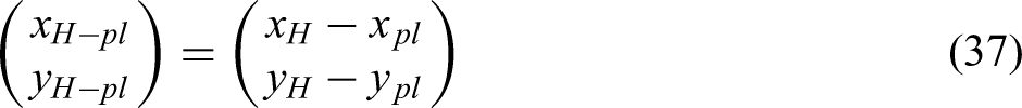

$$\left(\begin{array}{c}{x}_{H-pl}\\ y_{H-pl}\end{array}\right)=\left(\begin{array}{c}{x}_H-x_{pl}\\ y_H-y_{pl}\end{array}\right)$$

(37)

3-pendulum harmonograph initial condition

The initial conditions for the conical pendulum driving the platform motion is the same as that given for a 2-pendulum harmonograph.

The initial condition for the conical pendulums driving the pen is more complex than for a 2-pendulum harmonograph. The pen location in the x-y plane is denoted (x_H, y_H). The location of the extensions of the pendulums, (L_px,2, L_py,2) projected onto the x-y plane, are labelled (R + x_px, y_px) and (x_py, R + y_py), see Figures 2 and 7. When specifying the initial conditions for the conical pendulums controlling the pen, this is done as a three-stage process. The location of (x_H,0, y_H,0) using the ellipse specification (20), from this the coordinates, (x_px,0, y_px,0) and (x_py,0, y_py,0) are determined and then the pendulum conditions are calculated, (θ_px,0, φ_px,0, θ_py,0, φ_py,0) (23, 24).

The difficulty with the initial condition specification is the mapping from (x_H,0, y_H,0) to (x_px,0, y_px,0) and (x_py,0, y_py,0). The starting point for this is the kinematic equations,

$$(x_{H,0}-(R+x_{px,0}){)}^2+(y_{H,0}-y_{px,0}{)}^2=R^2$$

$$(x_{H,0}-x_{py,0}{)}^2+(y_{H,0}-(R+y_{py,0}){)}^2=R^2$$

(38)

This is a two-equation nonlinear solution in four unknowns so there is no unique solution. The best that can be done is to find a solution that is consistent with the conical pendulum conditions. Two constrained optimisation problems are specified such that (38) is satisfied, and the conical pendulum initial conditions exist. This is guaranteed if the following inequalities are satisfied.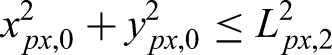

$$x_{px,0}^2+y_{px,0}^2\le L_{px,2}^2$$

$$x_{py,0}^2+y_{py,0}^2\le L_{py,2}^2$$

(39)

The two constrained optimisation problems are similar so only one is described. The initial conditions for the conical pendulum with the pendulum gimble located at (R,0) will be specified. The constrained optimisation problem is formulated using a penalty method, ¹⁴

$$f_{obj,px}=({(x_{H,0}-(R+x_{px,0}))}^2+{(y_{H,0}-y_{px,0})}^2-R^2{)}^2$$

$$f_{pen,px}={\alpha }_{pen}max\{0,x_{px,0}^2+y_{px,0}^2-L_{px,2}^2\}$$

$$f_{obj}=f_{obj,px}+f_{pen,px}$$

(40)

The constant α_pen is given a positive value such that the penalty function ensures that the solution satisfies (39). A numerical investigation of an appropriate value for α_pen suggests that any positive value is acceptable. The constrained optimisation problem is solved using a quasi-Newton method, using a BFGS update of the approximation to the Jacobian.^15,16

The initial velocities of the pendulum extensions are given by,

$${\dot{x}}_{px,0}={\dot{x}}_{H,0}$$

$${\dot{y}}_{px,0}={\dot{y}}_{H,0}$$

$${\dot{x}}_{py,0}={\dot{x}}_{H,0}$$

$${\dot{y}}_{py,0}={\dot{y}}_{H,0}$$

The initial conditions for the conical pendulums controlling the pen are,

$${\phi }_{px,0}={\tan }^{-1}\left({\displaystyle \frac{y_{px,0}}{x_{px,0}}}\right)$$

$${\theta }_{px,0}={\sin }^{-1}\left({\displaystyle \frac{x_{px,0}}{\cos {\phi }_{px,0}}}\right)$$

$$\left(\begin{array}{c}{\dot{x}}_{px,0}\\ {\dot{y}}_{px,0}\end{array}\right)=L_{px,2}\left(\begin{array}{cc}-\sin {\phi }_{px,0}\sin {\theta }_{px,0}& \cos {\phi }_{px,0}\cos {\theta }_{px,0}\\ \cos {\phi }_{px,0}\sin {\theta }_{px,0}& \sin {\phi }_{px,0}\cos {\theta }_{px,0}\end{array}\right)\left(\begin{array}{c}{\dot{\phi }}_{px,0}\\ {\dot{\theta }}_{px,0}\end{array}\right)$$

(41)

The initial conditions for the conical pendulum with its gimble located at (0, R) are specified in a similar way.

3-pendulum simulations

For a 3-pendulum harmonograph there are even more parameters defining the simulations than for a 2-pendulum harmonograph. This means that in this paper only a very small region of parameter space can be investigated.

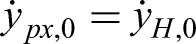
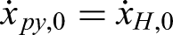
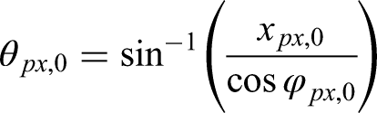
One of the attractions of a harmonograph is the observation of the development of a geometric design. Figure 8 shows the evolution of a 3-pendulum rotary harmonograph simulation. A geometric design defined in Table 1; Test 10 is shown in Figure 8. For Test 10 the natural frequencies of the three pendulums are, (ω_px, ω_py, ω_pl) = (3.99, 3.99,4.01) rad/s. Figure 8 is separated into four sub-figures showing the evolution of the geometric design at four times, Figure 8(a), t_frame = 25 s, Figure 8(b), t_frame = 50 s, Figure 8(c), t_frame = 100 s and Figure 8(d), t_frame = 200 s. In Figure 8(a) the initial pen trajectory is elliptical initially. For later times, Figure 8(b)–(d) the pen trajectory evolves into a very complex pattern, that is not easily described. An interesting point to note is it is not possible to determine the later time trajectory of the pen by inspecting the early time pen trajectory.

Figure 8.

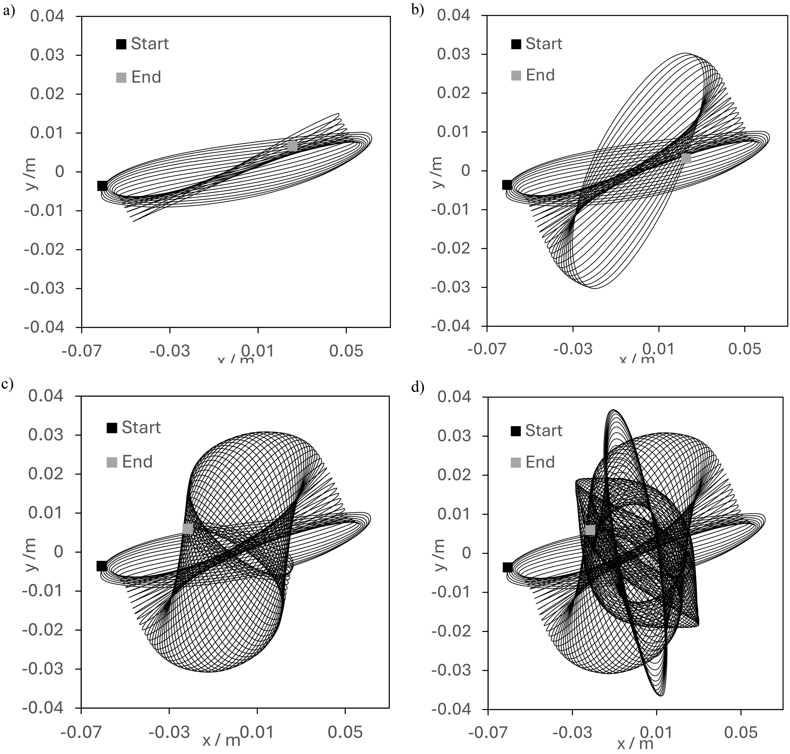
Geometric design produced for Test 10, (ω_pe,x, ω_pe,y, ω_pl) = (3.99, 3.99, 4.01), (a) t_frame = 25 s (b) t_frame = 50 s, (c) t_frame = 100 s and (d) t_frame = 200 s.

It is interesting to introduce frictional losses to Test 10. Test 11 is the same specification as Test 10 except K_f = 0.001 Ns/rad. Figure 9 shows the geometric pattern produced for the Test 11 specification, this should be compared with Figure 8(d), Test 10 at the same time, t_sim = 200 s. Figures 8(a) and 9 show that as expected the initial trajectories for Test 10 and Test 11 are near identical, but for later times a very different trajectory evolves for Test 11 compared to Test 10. The two figures show that introducing friction changes the long-time dynamics of the system, similar to the 2-pendulum harmonograph simulations, Figure 5(a), Test 5 and Figure 5(b), Test 6.

Figure 9.

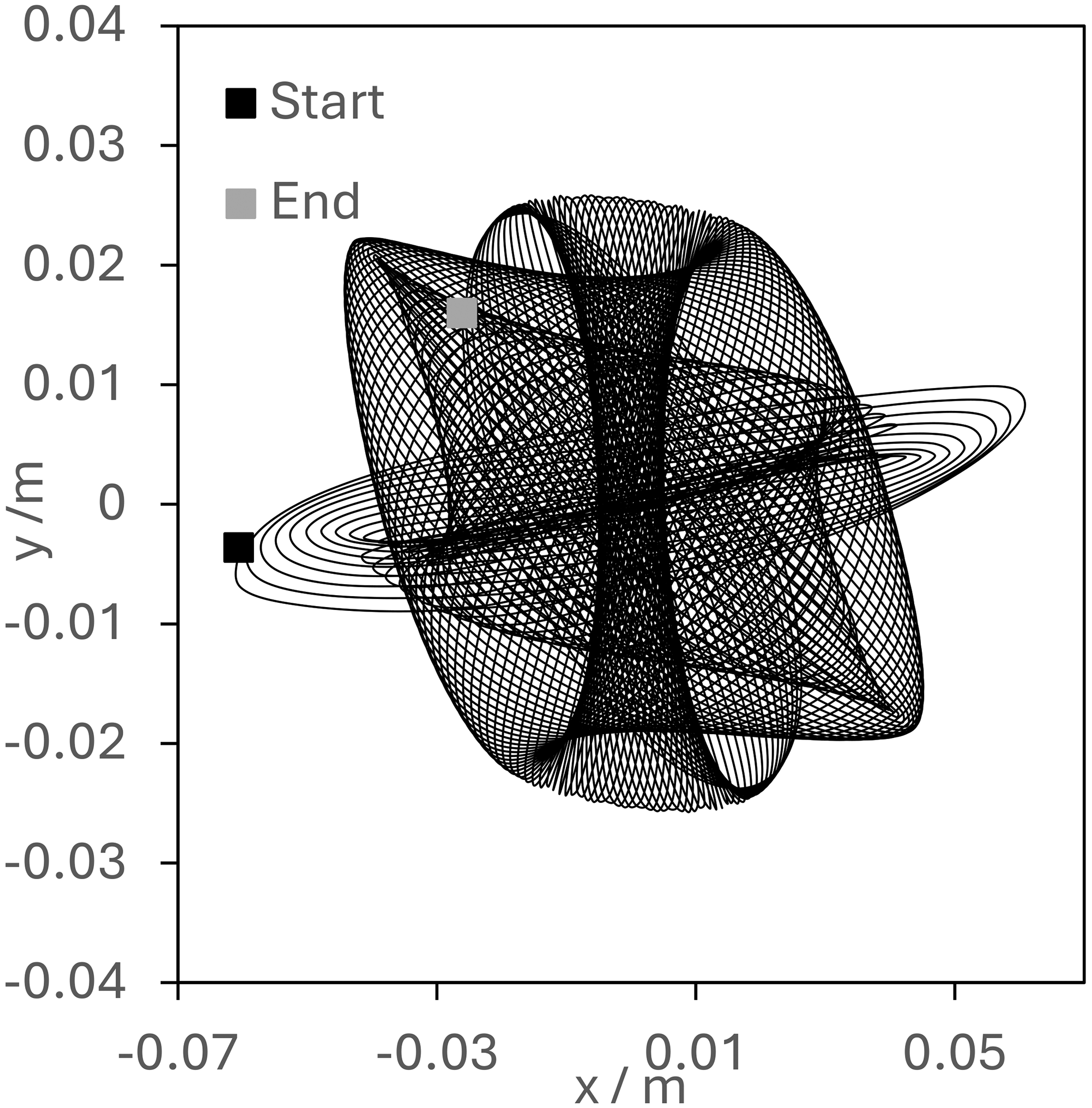
Geometric design produced for Test 11, (ω_pe,x, ω_pe,y, ω_pl) = (3.99, 3.99, 4.01), K_f = 0.001 Ns/rad.

The final two simulations, Test 12 and Test 13 show how sensitive the pen trajectory is to the perturbation of the natural frequencies in a 3-pendulum harmonograph. For Test 12 the natural frequencies of the harmonograph are,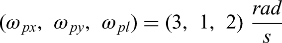

$$({\omega }_{px},{\omega }_{py},{\omega }_{pl})=(3,1,2){\displaystyle \frac{rad}{s}}$$

For Test 13 the natural frequencies are,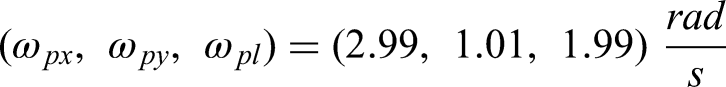

$$({\omega }_{px},{\omega }_{py},{\omega }_{pl})=(2.99,1.01,1.99){\displaystyle \frac{rad}{s}}$$

All other specifications of Test 12 and Test 13 are the same and given in Table 1. Comparing Figure 10(a), Test 12 and Figure 10(b), Test 13 the overall shape is similar but there are significant differences. Exploring the internet for images produced by physical harmonographs, ¹⁷ suggest that the natural frequencies of many physical harmonographs are close to, but not exact integer values.

Figure 10.

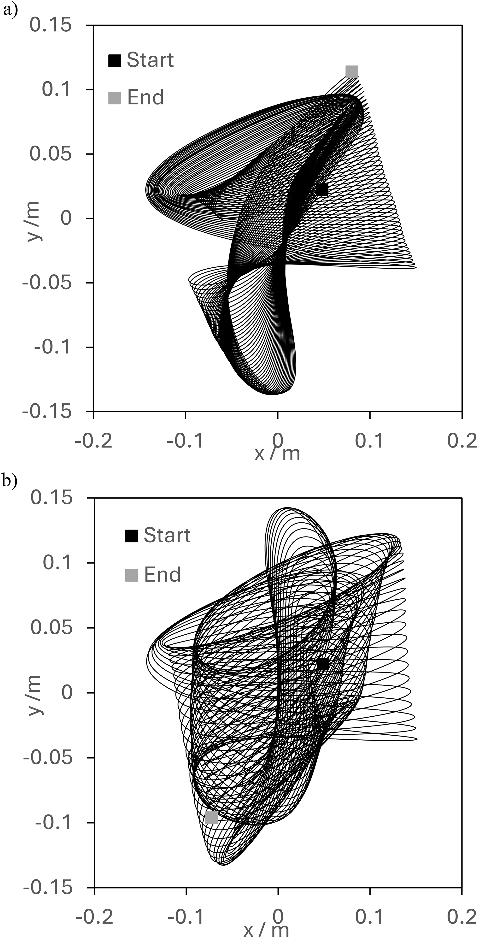
Geometric design produced for a) Test 12, (ω_px, ω_py, ω_pl) = (3, 1, 2), b) Test 13, (ω_px, ω_py, ω_pl) = (2.99, 1.01, 1.99).

Enhancing the student experience

The rotary harmonograph model can be used to enhance the student experience of undergraduate engineering students in much the same way as the lateral harmonograph model. ⁴ The rotary harmonograph is an excellent model for showing the interplay between natural frequencies of pendulums and friction producing interesting dynamic behaviour.

The author has demonstrated the conical pendulum model as a basis for a rotary harmonograph to students registered for an introductory course in dynamics. From discussions with the students taking the dynamics course, the students find the model very engaging and a motivation for maintaining interest in mechanical engineering science. The rotary harmonograph model is ideal for combining with a graphical user interface (GUI) in a programming environment such as MATLAB and handing the composite software over to the student body. Equipped with the software students can then explore parameter space of the harmonograph model with minimal supervision. As discussed above, one of the attractive features of the harmonograph model is to follow the evolution of a geometric design as it is produced, see Figure 8. Rather than producing a geometric design at different times the evolution of the design is possible in MATLAB using the comet function rather than the plot function.

Conclusion

In this paper a mathematical model for a rotary harmonograph is presented and analysed. The model can simulate a harmonograph with two or three pendulums. For the two pendulum harmonograph, one pendulum drives the pen and the second rotates the platform. For the more complex three pendulum harmonograph the motion of the pen is controlled by two pendulums. The harmonograph and initial condition specification defines a high dimensional parameter space. As a consequence, only a small region of parameter space is explored. In this paper the sensitivity of the geometric pattern generated to a number of different parameters is investigated. The parameters investigated are the harmonograph initial conditions, friction, and the natural frequencies of the pendulums.

For any geometric design produced by a harmonograph it is of interest to determine if it is possible to calculate initial conditions or approximate initial conditions. One conclusion of this investigation is that the sensitivity of the geometric design produced to the natural frequencies of the pendulums and the frictional loss in the system means that this is unlikely to be achieved, if not impossible.

Considering future directions of research in the modelling of harmonographs, in ⁴ an initial circular path or an Archimedean spiral is used to determine initial conditions for the pen. In this paper the initial conditions are determined based on a circular or elliptical curve. The rotary harmonograph with these initial conditions has produced a number of interesting geometric patterns. In the future there is value in the exploration of the patterns generated for diverse initial conditions. A good place to start would be to use (2) with d_x = d_y = 0 as a function for generating the initial pen and platform trajectory and velocity.

The rotary harmonograph model presented here and the lateral harmonograph model given in ⁴ means that it is possible to simulate the different types of harmonographs that are based on a combination of simple pendulums and conical pendulums, see Table 3. The next stage in the investigation is to produce a software tool that can simulate the different harmonographs defined in Table 3. The different harmonograph models can be embedded in a GUI. The harmonograph simulator software tool can then be handed over to mechanical engineering undergraduate students of dynamics to allow them to “go play” and express their artistic bent.

Table 3.

Different combinations of pendulums to produce different types of harmonograph.

		Pen
		1S	1C	2S	2C	1S 1C
Platform	0	-	-	X	X	X
	1 S	X	X	X	X	X
	1 C	X	X	X	X	X

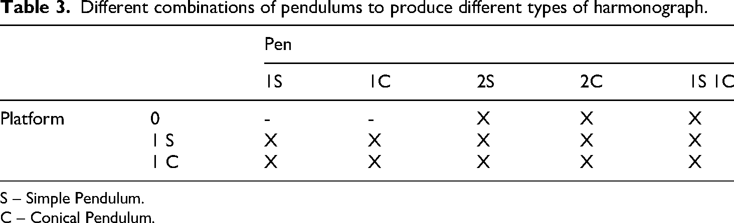
S – Simple Pendulum.

C – Conical Pendulum.