Sage Journals: Discover world-class research

Abstract

When a vehicle is driving, the most significant source of oscillations is the irregularities in the surface of the road. An active suspension is utilized to enhance the vehicle’s stability and ride comfort. In this work, the dynamic model with multi variables is considered to simulate vehicle oscillations based on four excitation cases from the road surface. In addition, this research also established the AFSP complex control solution for an active suspension system. This is a completely novel algorithm with many outstanding advantages. The final control signal of the system is synthesized from the signals of the linear controller PI (Proportional – Integral) and the nonlinear controller SMC (Sliding Mode Control). The controller’s parameters will change continuously depending on the established fuzzy rule. According to simulation outcomes, the vehicle body displacement and acceleration dramatically declined when the AFSP algorithm directed an active suspension. The values of acceleration and displacement do not exceed 80% and 20%, compared to the scenario in which the vehicle just utilized the typical passive suspension system. Besides, a phenomenon of “chattering” also does not appear when combining the controllers. Overall, the efficiency of this algorithm is high. This algorithm can be applied to more complex models.

Keywords

Active suspension system AFSP algorithm oscillation simulation vehicle dynamics vibration and noise control

Introduction

The stimuli on the road are the most essential reason for oscillations for the vehicle when moving. These oscillations can negatively impact passengers, cargo, and the life of the automobile. The suspension system is utilized to ensure that an automobile’s oscillations do not exceed the limit threshold.¹ Suspension systems used in automobiles are diverse, such as mechanical suspension (passive suspension), active suspension, semi-active suspension, and pneumatic suspension.² A conventional mechanical suspension system has a basic structure and a low price and is now used on most popular cars. Typical components of a mechanical suspension system include coil springs (or leaf springs, torsion bars), dampers, and lever arms (upper arm and/or lower arm).³ Besides, the stabilizer bar can also be considered a suspension system component.⁴ The passive suspension system can only meet the oscillation requirements under normal conditions. In special situations, loss of ride comfort can occur if an automobile utilizes only this suspension system. Its property is constant (fixed) for a conventional passive suspension, although the characteristic curves of the components can be linear or nonlinear. Therefore, it cannot respond to constantly changing external stimuli. To improve this, an air suspension system with air springs, which can change stiffness using internal compressed air pressure, was used.^5,6 In addition, a semi-active suspension with the MR damper is also used to better adapt to oscillations from the road surface.^7,8 One of the most effective methods of responding to vehicle oscillation requirements is the use of an active suspension.⁹ According to Omar et al., an active suspension’s actuator has the form of a hydraulic cylinder. The cylinder inside contains the servo-valve, which is driven via the control voltage signal.¹⁰ An impact force produced by a hydraulic actuator will act on both masses of an automobile (for some other suspension systems, the actuator may be electromagnetic). So, the oscillation of a vehicle will decrease gradually.¹¹

Many studies on control problems for active suspension systems have been introduced in the last few decades. Trang and Lan¹² used PID (Proportional – Integral – Derivative) algorithm to control this system. This controller includes three stages corresponding to three coefficients, K_D, K_P, and K_I.¹³ These coefficients will be self-tuning or selected based on Ziegler–Nichols’s method.¹⁴ However, the effectiveness of these methods is often low. Chen and Zhou¹⁵ used the Fuzzy algorithm to tune the PID controller’s variables based on excitation signals from the road. Based on the principle of genetics, the variables of the PID controller can be optimally chosen by the GA (Genetic Algorithm) solution. This was done by Metered et al.¹⁶ The size of the population and the number of generations will be determined based on the experience of the designer.¹⁷ Different from the GA algorithm, the PSO (Particle Swarm Optimization) method helps optimize the controller’s coefficients based on the characteristics of the animals.¹⁸ The animals used in this algorithm often have a herd lifestyle, such as whales, ants, bees, etc.^19–21 Besides, many other intelligent algorithms have been used to search for the controller’s parameters optimally.^22–24 The PID controller can only be applied to systems that have an object. If the system has many objects to be controlled, using multiple PID controllers is a suitable alternative.²⁵ For MIMO (Multi Input – Multi Output) systems, the Linear – Quadratic Regulator (LQR) controller can be used to replace the conventional PID controller.²⁶ This algorithm aims to minimize the cost function so the system can be more stable.²⁷ The mathematical model of this algorithm must be given in the form of a state matrix.²⁸ Once the Gaussian filter is combined with the LQR controller, it will be called an LQG (Linear – Quadratic Gaussian) controller.²⁹ The above methods are only used for linear objects. If the object is nonlinear, more complex algorithms need to be used.

The SMC algorithm is often used for complex nonlinear objects.³⁰ Kazemian et al.³¹ used the SMC algorithm to control the hydraulic actuator. To simplify the model, a linearization process of a hydraulic actuator should be done. This process is shown by Nguyen.³² Then, a quarter-dynamic model that considers the influence of the actuator will have five state variables.³³ According to Zhao et al.,³⁴ the sliding surface is an important component of the SMC controller. The controlled object can travel around the sliding surface in order to reach a steady state.³⁵ Notwithstanding, a “chattering” phenomenon can occur when this algorithm is used. This problem can make the control signal vibrate continuously with high frequency and a small amplitude.^31,36 To limit this problem, a SMC controller must be combined with a PID controller or a Fuzzy controller.³⁷ For instance, Hsiao and Wang³⁸ introduced the design of an algorithm that combines SMC and Fuzzy, called STFSMC (Self-tuning Fuzzy Sliding Mode Controller). Another recommendation has been made by Suhail et al.³⁹ about using the ASMC (Adaptive Sliding Mode Control) algorithm. Overall, ride comfort can be greatly improved if this method is used.^40,41 Besides, many advanced control methods have been applied to the active suspension system, which also brings high efficiency.^42–45

In this paper, vehicle oscillation is simulated using a quarter dynamic model. Besides, a hydraulic actuator is also considered in this model. To enhance the system’s stability, the AFSP integration algorithm is used. This is a new control algorithm that was proposed by the author. According to this proposal, the integrated controller’s control signal is synthesized between SMC and PI controllers. Moreover, the parameters of the PI controller are adjusted by a Fuzzy algorithm to respond to continuously changing external stimuli. So, it can work well even if the excitation from the pavement is linear or nonlinear. As a result, the efficiency in ensuring the stability and comfort of the vehicle when moving will be enhanced. This is considered a novel point in the paper, which brings some significant contributions to the field of automotive suspension control. The calculations and simulation are done by the MATLAB application. The main content of this work includes of four sections: introduction, method, results and discussions, and conclusions. These will be presented in the next sections.

Method

Vehicle model

A dynamic model needs to be established to simulate vehicle oscillations. This model consists of a sprung mass m₁ and an unsprung mass m₂ (Figure 1). There are two DOFs corresponding to the two masses, z₁, and z₂. The hydraulic actuator is responsible for generating the force F_A.

F_{i}^{m_{1}} = F_{A} + F_{K} + F_{C}

(1)

F_{i}^{m_{2}} = - F_{K} - F_{A} - F_{C} + F_{KT}

(2)

Where:

Inertia force:

F_{i}^{m_{i}} = m_{i} {\overset{\cdot\cdot}{z}}_{i}

(3)

Spring force:

F_{K} = - K (z_{1} - z_{2})

(4)

Damping force:

F_{C} = - C ({\overset{\cdot}{z}}_{1} - {\overset{\cdot}{z}}_{2})

(5)

Tire force:

F_{KT} = - K_{T} (z_{2} - h)

(6)

Figure 1.

A quarter dynamics model.

According to Nguyen,³² the impact force produced by an actuator can be simplified as follows:

{\overset{\cdot}{F}}_{A} = γ_{1} i (t) - γ_{2} F_{A} - γ_{3} ({\overset{\cdot}{z}}_{1} - {\overset{\cdot}{z}}_{2})

(7)

Let five variables:

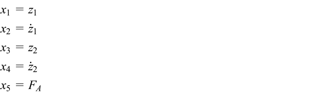
\begin{matrix} x_{1} = z_{1} \\ x_{2} = {\overset{\cdot}{z}}_{1} \\ x_{3} = z_{2} \\ x_{4} = {\overset{\cdot}{z}}_{2} \\ x_{5} = F_{A} \end{matrix}

Taking into account the state variables’ derivatives:

\begin{matrix} {\overset{\cdot}{x}}_{1} = x_{2} \\ {\overset{\cdot}{x}}_{2} = \frac{1}{m_{1}} (- K x_{1} - C x_{2} + K x_{3} + C x_{4} + x_{5}) \\ {\overset{\cdot}{x}}_{3} = x_{4} \\ {\overset{\cdot}{x}}_{4} = \frac{1}{m_{2}} [K x_{1} + C x_{2} - (K + K_{T}) x_{3} - C x_{4} - x_{5}] \\ x_{5} = - γ_{3} x_{2} + γ_{3} x_{4} - γ_{2} x_{5} + γ_{1} i (t) \end{matrix}

The following is a description of the matrix that characterizes the oscillations of the system:

\begin{matrix} [\begin{matrix} \begin{matrix} {\overset{\cdot}{x}}_{1} \\ {\overset{\cdot}{x}}_{2} \end{matrix} \\ {\overset{\cdot}{x}}_{3} \\ {\overset{\cdot}{x}}_{4} \\ {\overset{\cdot}{x}}_{5} \end{matrix}] = [\begin{matrix} 0 & 1 & 0 & 0 & 0 \\ - \frac{K}{m_{1}} & - \frac{C}{m_{1}} & \frac{K}{m_{1}} & \frac{C}{m_{1}} & \frac{1}{m_{1}} \\ 0 & 0 & 0 & 1 & 0 \\ \frac{K}{m_{2}} & \frac{C}{m_{2}} & - \frac{K + K_{T}}{m_{2}} & - \frac{C}{m_{2}} & - \frac{1}{m_{2}} \\ 0 & - γ_{3} & 0 & γ_{3} & - γ_{2} \end{matrix}] [\begin{matrix} \begin{matrix} x_{1} \\ x_{2} \end{matrix} \\ x_{3} \\ x_{4} \\ x_{5} \end{matrix}] \\ + [\begin{matrix} \begin{matrix} 0 \\ 0 \end{matrix} \\ 0 \\ 0 \\ γ_{1} \end{matrix}] i (t) + [\begin{matrix} \begin{matrix} 0 \\ 0 \end{matrix} \\ 0 \\ \frac{K_{T}}{m_{2}} \\ 0 \end{matrix}] h (t) \end{matrix}

(8)

After the dynamic model describing the vehicle oscillation has been established, the control algorithm also needs to be designed.

Control model

Considering the indeterminate SISO nonlinear system, let u(t) be the input signal and y(t) the output signal. An input-output model is described below:

y^{(n)} = f (y, \overset{\cdot}{y}, \overset{\cdot\cdot}{y}, . . ., y^{(n - 1)}) + u (t)

(9)

Symbols for state variables:

x_{k} = y^{(k - 1)}; k = \bar{1, n}

(10)

Then, the equation (9) is rewritten as (11) where f( x ) is an uncertain function.

{\begin{matrix} {\overset{\cdot}{x}}_{k} = x_{k + 1}; 1 \leq k \leq n - 1 \\ {\overset{\cdot}{x}}_{n} = f (\underline{x}) + u (t) \end{matrix} \underline{x} = [\begin{matrix} x_{1} \\ x_{2} \\ . . . \\ x_{n} \end{matrix}]

(11)

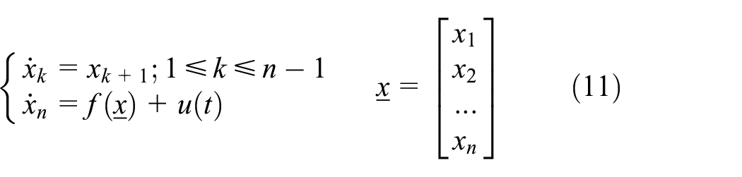
The function f( x ) is limited, that is:

| f (\underline{x}) | \leq φ (\underline{x}), \forall x

(12)

When t > 0, the controller ensures that the closed system always has a free-state orbital x(t) with a limit. If the setpoint is zero, that is:

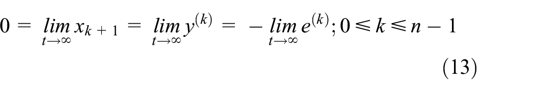
0 = \lim_{t \to \infty} x_{k + 1} = \lim_{t \to \infty} y^{(k)} = - \lim_{t \to \infty} e^{(k)}; 0 \leq k \leq n - 1

(13)

Where: e(t) is the error signal between the setpoint signal and the output signal.

e (t) = y_{s} (t) - y (t)

(14)

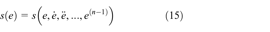
Assume that s(e) is a smooth function. This function will depend on error signals e(t) of the system.

s (e) = s (e, \overset{\cdot}{e}, \overset{\cdot\cdot}{e}, . . ., e^{(n - 1)})

(15)

If the solution e(t) of the equation s(e) = 0 satisfies the condition (13), the function s(e) is called a sliding surface (Figure 2).

s (e) = 0

(16)

Figure 2.

Sliding surface.

To simplify the problem, a constant parametric linear sliding surface is often used. Considering the sliding surface given in (17):

\begin{matrix} s (e) = k_{0} + k_{1} \overset{\cdot}{e} + k_{2} \overset{\cdot\cdot}{e} + . . . + k_{n - 2} e^{(n - 2)} + e^{(n - 1)} = k_{0} \\ + \sum_{i = 1}^{n - 2} k_{i} e^{(i)} + e^{(n - 1)} \end{matrix}

(17)

The roots of the equation (16) satisfy condition (13) if and only if coefficients k_i of the equation (17) are the constants of the polynomial p(λ). Also, the polynomial p(λ) must be a Hurwitz polynomial.

\begin{matrix} p (λ) = k_{0} + k_{1} λ + k_{2} λ^{2} + . . . + k_{n - 2} λ^{n - 2} + λ^{n - 1} = k_{0} \\ + \sum_{i = 1}^{n - 2} k_{i} λ^{i} + λ^{n - 1} \end{matrix}

(18)

For the system in order to be asymptotically stable, the sliding surface s(e) must approach zero, that is:

sgn (s) \overset{\cdot}{s} < 0

(19)

According to (11), (17), and (19), we have:

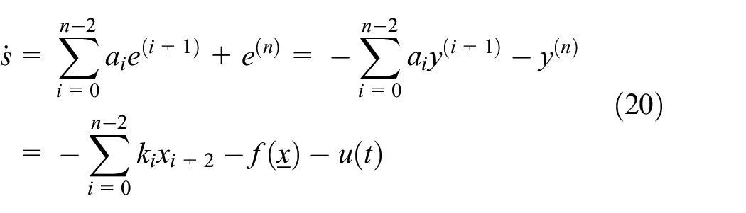
\begin{matrix} \overset{\cdot}{s} = \sum_{i = 0}^{n - 2} a_{i} e^{(i + 1)} + e^{(n)} = - \sum_{i = 0}^{n - 2} a_{i} y^{(i + 1)} - y^{(n)} \\ = - \sum_{i = 0}^{n - 2} k_{i} x_{i + 2} - f (\underline{x}) - u (t) \end{matrix}

(20)

Condition (19) is rewritten as follows:

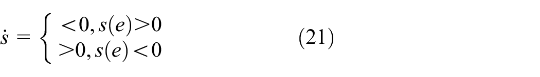
\overset{\cdot}{s} = {\begin{matrix} < 0, s (e) > 0 \\ > 0, s (e) < 0 \end{matrix}

(21)

Combining (20) and (21), the sliding condition of the controller is shown in the formula (22).

u (t) = {\begin{matrix} > - \sum_{i = 0}^{n - 2} k_{i} x_{i + 2} - f (\underline{x}), s (e) > 0 \\ < - \sum_{i = 0}^{n - 2} k_{i} x_{i + 2} - f (\underline{x}), s (e) < 0 \end{matrix}

(22)

In order to improve the system’s stability, the sliding mode controller will be combined with a PID controller. The PID controller includes three basic elements: proportional, integral, and derivative. Let v(t) be the input signal and q(t) the error signal of the system. The control signal of the PID controller is illustrated below.

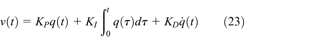
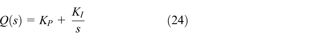
v (t) = K_{P} q (t) + K_{I} \int_{0}^{t} q (τ) d τ + K_{D} \overset{\cdot}{q} (t)

(23)

The higher-order derivative signal can cause some unwanted disturbances. Therefore, this signal should be discarded if it is not needed. If the derivative stage is ignored, a transfer function of the system can be rewritten as (24):

Q (s) = K_{P} + \frac{K_{I}}{s}

(24)

The control signal of the integrated controller is determined based on the combination of the PI controller and the SMC controller.

i (t) = u (t) + v (t)

(25)

Figure 3 presents a control system diagram. To help the system respond well to the continuous change of external stimuli, the coefficients of the PI controller are adjusted by the fuzzy algorithm. According to the fuzzy theory, an intermediate state can exist to better respond to the flexible change of oscillation states. The membership function of the fuzzy controller is illustrated in Figure 4. Many views deal with the problem of selecting and establishing the membership function for the system. The membership function that is used in this research is established by the author based on some opinions as follows:

+ In the vehicle’s state with small oscillations (ξ₃÷ξ₄), the control signal needs to be small or non-existent.

+ When the car vibrates more strongly (ξ₁÷ξ₃ or ξ₄÷ξ₆), the control signal must be changed accordingly (increase or decrease).

+ The membership function values will be re-calibrated after each test simulation to give suitable final values.

Figure 3.

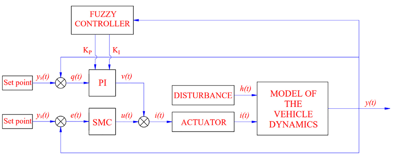
Schematic of the AFSD algorithm.

Figure 4.

Membership function.

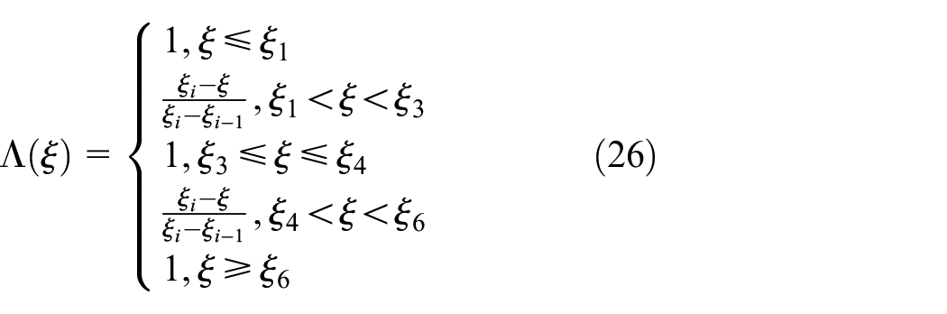
The defuzzification process is performed according to the rules as shown in the equation (26).

\begin{matrix} Λ (ξ) = {\begin{matrix} 1, ξ \leq ξ_{1} \\ \frac{ξ_{i} - ξ}{ξ_{i} - ξ_{i - 1}}, ξ_{1} < ξ < ξ_{3} \\ 1, ξ_{3} \leq ξ \leq ξ_{4} \\ \frac{ξ_{i} - ξ}{ξ_{i} - ξ_{i - 1}}, ξ_{4} < ξ < ξ_{6} \\ 1, ξ \geq ξ_{6} \end{matrix} \end{matrix}

(26)

Once the integrated controller has been designed, simulation should be carried out. MATLAB-Simulink is the environment in which this procedure is carried out.

Result and discussion

Conditions

In this work, the oscillation source is the road surface excitation. While moving down a road, a vehicle may come into contact with various forms of stimuli. To simulate oscillations comprehensively, this paper uses four excitation types, as shown in Figure 5. These are common excitation forms commonly used in oscillation and control problems for suspension systems. Equation (27) describes the pavement excitation for the first case and the second case, while equations (28) and (29) describe pavement excitation for the other two cases in order.

h (t) = h_{0} \sin (2 π ft + φ)

(27)

h (t) = {\begin{matrix} 0, t < t_{0} \\ h_{0} \frac{t - t_{0}}{τ_{1}}, t_{0} \leq t < t_{0} + τ_{1} \\ h_{0}, t_{0} + τ_{1} \leq t < t_{0} + τ_{2} \\ 0, t \geq t_{0} + τ_{3} \end{matrix}

(28)

h (t) = 2 π \int_{0}^{t} [- fh (τ) + \sqrt{Gv ω (τ)}] d τ

(29)

Where:

h ₀: Amplitude of oscillation

f: Frequency of oscillation

φ: Initial phase

G: constant

ω: White noise signal

Figure 5.

Bump on the road: (a) first case, (b) second case, (c) third case, and (d) fourth case.

In the first two cases, the pavement excitation frequency and amplitude differ. This is to investigate the car’s oscillations when faced with different stimuli. In the third case, a trapezoidal pulsed excitation is used. The excitation acceleration will be much larger than in the above two cases. Therefore, this case is utilized to evaluate the smoothness of the vehicle when suddenly encountering single-pulse stimuli. Finally, a case involving random stimulation is used. This type of excitation has a high amplitude and frequency and is considered a realistic description of the road surface. The random excitation is generated from a white noise signal source, which is described by the equation (29).

In each case, three situations were examined: an automobile utilizing an active suspension with the AFSP algorithm, an automobile utilizing an active suspension system with the SMC control algorithm, and an automobile utilizing a mechanical suspension system.

The specifications used for a simulation are illustrated in Table 1. The γ₁, γ₂, and γ₃ coefficients are referenced from Nguyen and Nguyen.³³

Table 1.

Reference coefficients.

Notation	Description	Value	Unit
m ₁	Sprung mass	500	kg
m ₂	Unsprung mass	55	kg
C	Damper coefficient	3900	Ns/m
K	Spring coefficient	45,000	N/m
K_T	Tire coefficient	180,000	N/m
γ ₁	Actuator coefficient	539,561	N^3/2/kg^1/2m^1/2V
γ ₂	Actuator coefficient	1	s⁻¹
γ ₃	Actuator coefficient	5,512,500	N/m

Simulation result

Case 1

Within the first scenario, a sine-shaped pavement is used. This is a cyclic excitation with a small amplitude and frequency. Therefore, the vehicle oscillation also varies periodically according to this excitation signal.

The variation in the vehicle body displacement over time is seen in Figure 6. The vehicle body displacement is the largest when an automobile only uses the passive suspension, reaching 54.09 mm. Displacement will be reduced if the car uses the active suspension mentioned above. The maximum values for the other two situations are 24.03 and 10.83 mm, respectively. The changing trend of all three curves is similar to that of the excitation signal from the road surface. For continuous oscillations, the mean value should be considered. This value is determined according to the RMS (Root Mean Square) of three situations: an automobile has an active suspension with an AFSP controller, an automobile has an active suspension with the SMC controller, and an automobile has only a mechanical suspension system, reaching 7.58, 16.82, and 37.31 mm. This difference is quite large.

Figure 6.

The change of displacement (sprung mass).

The value of a vehicle body’s acceleration is able to be used to measure the oscillations of the automobile. A change in acceleration is shown in Figure 7. In the first phase, the acceleration is very large, reaching 0.46, 0.66, and 0.81 m/s², respectively, with three situations examined. This value will gradually decrease and oscillate periodically in the following phases. When an active suspension system is utilized on the automobile with the AFSP algorithm, the mean acceleration value is only 26.32% compared to the car using a conventional mechanical suspension system (100%) and an active suspension with the SMC algorithm (47.37%). So, the automobile’s smoothness has been significantly increased. Compared with the results in some previous studies,^46,47 the automobile’s oscillation simulated in this paper has a more accurate oscillation phase. In addition, the chattering phenomenon is almost non-existent compared to the results in Moghadam and Kebriaei.³⁶ This helps demonstrate the new algorithm’s positive performance, which is proposed in this study.

Figure 7.

The change of acceleration.

In some exceptional cases, the hydraulic actuator can generate a significant impact force, which causes instability of the unsprung mass. However, this did not happen once the AFSP algorithm was used to direct the active suspension. According to Figure 8, the displacement of the unsprung mass for all three situations is similar (the difference is tiny).

Figure 8.

The change of displacement (unsprung mass).

Case 2

In the above case, the oscillation is still quite small. Therefore, the stable performance of the system has not been fully determined yet. To determine this, oscillations of greater frequency and the amplitude need to be used. In the second case, the sine-shaped pavement continues to be used. However, the amplitude and frequency of the oscillations have been enhanced.

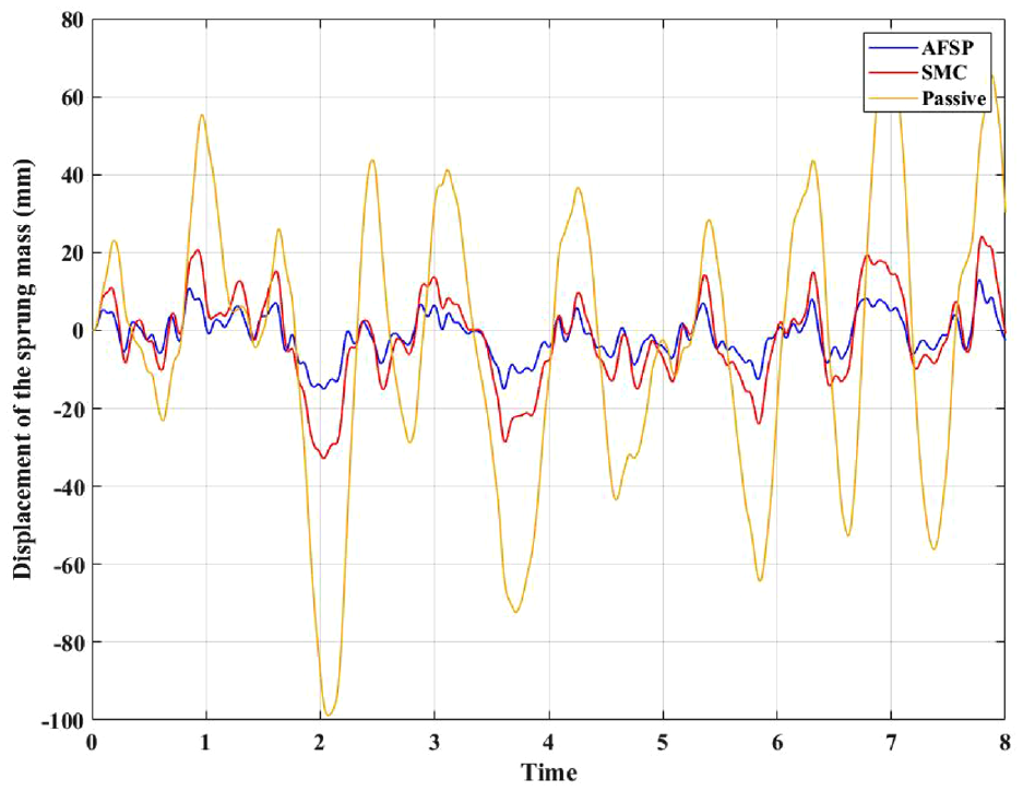
As the amplitude of the excitation increases, the sprung mass displacement value also increases rapidly (Figure 9). Like the case above, vehicle oscillation is minimal when the AFSP algorithm is used to control a modern suspension. Its maximum values and mean values are only 21.65 and 15.36 mm, respectively, only about 17.09% (126.66 mm) and 18.73% (82 mm) compared to a situation of an automobile utilizing a mechanical suspension. Meanwhile, the values obtained using the SMC algorithm are 48.07 and 33.96 mm, respectively, reaching 37.95% and 41.41%.

Figure 9.

The change of displacement (sprung mass).

A change in acceleration with time also tends to be similar to the case above (Figure 10). The maximum value and mean value determined according to the RMS criteria of three situations are: 1.35, 1.97, and 2.42 m/s²; 0.17, 0.35, and 0.84 m/s².

Figure 10.

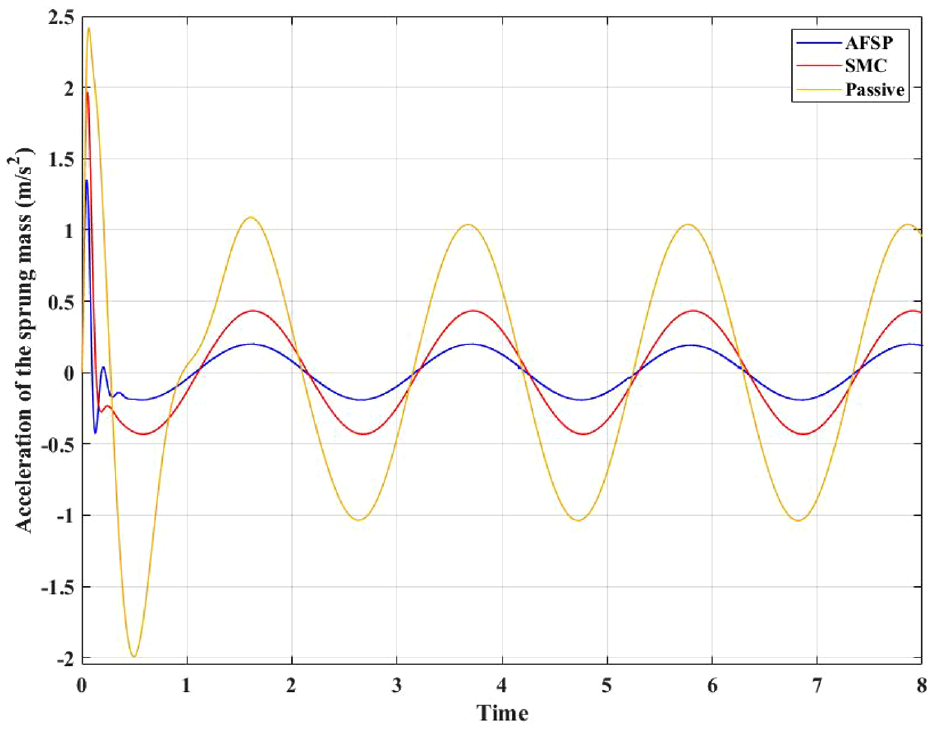
The change of acceleration.

Similar to the above case, the difference in the displacement of the unsprung mass in the second case is also very small (Figure 11). Besides, this value is slightly smaller if the car uses active suspension instead of passive suspension. In general, the smoothness and stability of the vehicle are always guaranteed.

Figure 11.

The change of displacement (unsprung mass).

Case 3

The control system is considered responsive if and only if the control signal appears and ends with the excitation signal (the time difference is extremely small). In some cases, when the excitation signal from the pavement has ended, the control signal is still maintained. This will cause system instability. To evaluate this responsiveness, a single pulsed excitation was used.

According to the results shown in Figure 12, the vehicle body will return to its original position as soon as the excitation signal ceases to exist if the automobile uses a modern suspension (including AFSP and SMC). In contrast, if a conventional suspension system is used, the vehicle body oscillation continues for a small amount of time, about 1.8 s. Besides, the maximum displacement and acceleration values greatly decline when an AFSP algorithm is used, reaching 21.65 mm and 1.35 m/s². Meanwhile, the values of the other two cases are 48.07 mm and 1.97 m/s² for SMC; 126.66 mm and 2.42 m/s² for passive. These findings are illustrated in Figures 12 and 13, respectively.

Figure 12.

The change of displacement (sprung mass).

Figure 13.

The change of acceleration.

The value of the displacement of the unsprung mass in the third case is completely followed by the excitation signal from the pavement. This value is almost no different, even when the car uses active or passive suspension (Figure 14).

Figure 14.

The change of displacement (unsprung mass).

Case 4

The roughness of the road is the random form in the last case. This is a common form when an automobile is traveling on the road. With this excitation form, the vehicle’s oscillations will change continuously at a quite high frequency and value. This can negatively affect the vehicle’s comfort.

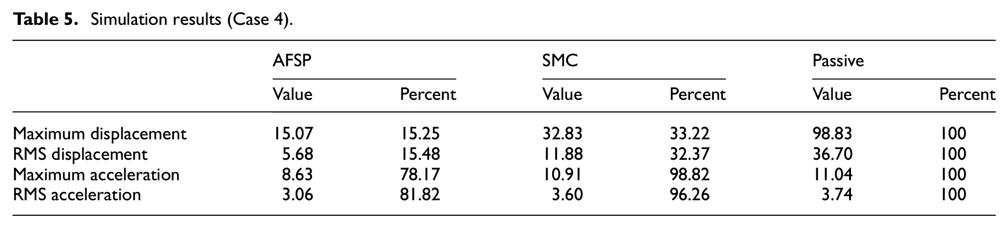
According to the findings presented in Figure 15, the maximum and mean values of the vehicle displacement when an automobile only utilizes the mechanical suspension are 98.83 and 36.70 mm. If an automobile uses an active suspension directed by the SMC algorithm, this value is reduced to 32.83 and 11.88 mm. These values can be further reduced if the AFSP solution is utilized to direct the hydraulic suspension system. These values can reach 15.07 and 5.68 mm. These are very small oscillations and do not affect the vehicle’s comfort when traveling.

Figure 15.

The change of displacement (sprung mass).

In this case, the vehicle body acceleration is very large (Figure 16). It can go up to 11.04, 10.91, and 8.63 m/s². The ride comfort can be better-guaranteed thanks to the modern active suspension system with the AFSP method.

Figure 16.

The change of sprung mass.

Finally, a result that describes the displacement of the unsprung mass is shown in Figure 17. In general, there is not a big difference between the situations. It can be understood that the oscillation of the unsprung mass will not be affected once the vehicle uses active suspension.

Figure 17.

The change of displacement (unsprung mass).

The outcomes of the calculation process are listed in Tables 2 to 5.

Table 2.

Simulation results (Case 1).

	AFSP		SMC		Passive
	Value	Percent	Value	Percent	Value	Percent
Maximum displacement	10.83	20.02	24.03	44.43	54.09	100
RMS displacement	7.58	20.32	16.82	45.08	37.31	100
Maximum acceleration	0.46	56.79	0.66	81.48	0.81	100
RMS acceleration	0.05	26.32	0.09	47.37	0.19	100

Table 3.

Simulation results (Case 2).

	AFSP		SMC		Passive
	Value	Percent	Value	Percent	Value	Percent
Maximum displacement	21.65	17.09	48.07	37.95	126.66	100
RMS displacement	15.36	18.73	33.96	41.41	82.00	100
Maximum acceleration	1.35	55.79	1.97	81.40	2.42	100
RMS acceleration	0.17	20.24	0.35	41.67	0.84	100

Table 4.

Simulation results (Case 3).

	AFSP		SMC		Passive
	Value	Percent	Value	Percent	Value	Percent
Maximum displacement	21.84	20.05	48.53	44.56	108.91	100
RMS displacement
Maximum acceleration	0.46	54.76	0.66	78.57	0.84	100
RMS acceleration

Table 5.

Simulation results (Case 4).

	AFSP		SMC		Passive
	Value	Percent	Value	Percent	Value	Percent
Maximum displacement	15.07	15.25	32.83	33.22	98.83	100
RMS displacement	5.68	15.48	11.88	32.37	36.70	100
Maximum acceleration	8.63	78.17	10.91	98.82	11.04	100
RMS acceleration	3.06	81.82	3.60	96.26	3.74	100

The percentage change of the values is given as shown in Figure 18.

Figure 18.

Percent of the values: (a) first case, (b) second case, (c) third case, and (d) fourth case.

Conclusion

Vehicle oscillations have an important influence on passenger comfort and the quality of the merchandise. Several factors might cause a vehicle to oscillate, but road surface irregularity is the most prominent factor contributing to this phenomenon. An active suspension with hydraulic actuators is utilized to enhance the automobile’s comfort when traveling. The system’s stability depends entirely on the control algorithm utilized to direct an active suspension.

This research uses the dynamic model with five state variables to describe vehicle oscillations. Where a hydraulic actuator is taken into account as one state variable of this model. The proposed AFSP algorithm is used for this model. This is a novel and complex model. The variables of the PI controller can be changed continuously by the fuzzy law. The control signal is determined based on the output signal of the PI controller and the SMC controller.

The findings of this research have shown the outstanding advantages of the AFSP solution. According to this result, the maximum values, as well as the mean values determined according to the RMS criteria of the sprung mass displacement and acceleration, have been greatly reduced compared to other investigated situations. In addition, the reaction of the control signal also follows the excitation signal from the road, which causes the automobile to oscillate. The automobile’s comfort and stability have been increased when the car utilizes the active suspension system with the AFSP control solution. The new contributions of this algorithm are entirely positive and help further to confirm the outstanding advantages of the AFSP algorithm.

Footnotes

Appendix

Handling Editor: Chenhui Liang

Declaration of conflicting interests

The author declared no potential conflicts of interest with respect to the research, authorship, and/or publication of this article.

Funding

The author received no financial support for the research, authorship, and/or publication of this article.

ORCID iD

Tuan Anh Nguyen

References

Kashem

SBA

Mustapha

Kannan

, et al. A study and review on vehicle suspension system and introduction of a high-bandwidth configured quarter car suspension system. Aust J Basic Appl Sci 2015; 9: 59–66.

Jiregna

Sirata

. A review of the vehicle suspension system. J Mech Energy Eng 2020; 4: 109–114.

Sename

. Review on LPV approaches for suspension systems. Electronics 2021; 10: 2120.

Nguyen

, et al. Enhancing the stability and safety of vehicle when steering by using the active stabilizer bar. Math Probl Eng 2022; 2022: 1–10.

Yin

Huang

Shangguan

, et al. Study on the influence of air suspension levelling valve charging and discharging characteristics on heavy truck roll stability. SAE technical paper 2021-01-0980, 2021.

Zhang

Wang

, et al. Semi-active control of air suspension with auxiliary chamber subject to parameter uncertainties and time-delay. Int J Robust Nonlin Control 2020; 30: 7130–7149.

Vivas-Lopez

Tudon-Martinez

Estrada-Vela

, et al. Damping variation effects in vehicle semi-active MR suspension: a stress concentration analysis. Front Mater 2021; 8: 590390.

Florean-Aquino

. Modern semi-active control schemes for a suspension with MR actuator for vibration attenuation. Actuators 2021; 10: 22.

Huang

, et al. Approximation-free control for vehicle active suspensions with hydraulic actuator. IEEE Trans Ind Electron 2018; 65: 7258–7267.

10.

Omar

El-kassaby

Abdelghaffar

. A universal suspension test rig for electrohydraulic active and passive automotive suspension system. Alex Eng J 2017; 56: 359–370.

11.

Sun

Zhao

. Adaptive neural network sliding mode control for active suspension systems with electrohydraulic actuator dynamics. Int J Adv Robot Syst 2020; 17: 172988142094198.

12.

Trang

Lan

DNH

. Modeling and simulation of PID controller-based active suspension system for a quarter car model. J Tech Educ 2022; 68: 111–120.

13.

Baltieri

Buckley

. PID control as a process of active inference with linear generative models. Entropy 2019; 21: 257.

14.

Huba

Chamraz

Bistak

, et al. Making the PI and PID controller tuning inspired by Ziegler and Nichols precise and reliable. Sensors 2021; 21: 6157.

15.

Chen

Zhou

. Modelling and analysis of automobile vibration system based on fuzzy theory under different road excitation information. Complexity 2018; 2018: 1–9.

16.

Metered

Abbas

Emam

. Optimized proportional integral derivative controller of vehicle active suspension system using genetic algorithm. SAE technical paper 2018-01-1399, 2018.

17.

Nagarkar

Bhalerao

Vikhe Patil

, et al. GA-based multi-objective optimization of active nonlinear quarter car suspension system – PID and fuzzy logic control. Int J Mech Mater Eng 2018; 13: 1–20.

18.

Al-Mutar

Abdalla

. Quarter car active suspension system control using PID controller tuned by PSO. Iraq J Electr Electron Eng 2015; 11: 151–158.

19.

Karam

Awad

. Design of active fractional PID controller based on whale’s optimization algorithm for stabilizing a quarter vehicle suspension system. Period Polytech Electr Eng Comput Sci 2020; 64: 247–263.

20.

Aldair

Abdalla

Alsaedee

. Design of PID controller using ABC for full vehicle nonlinear active suspension system with passenger seat. Int J Comput Appl 2017; 167: 18–27.

21.

Zhao

Zhu

. Multi-objective optimization of active suspension predictive control based on improved PSO algorithm. J Vibroengineering 2019; 21: 1388–1404.

22.

Dahunsi

Dangor

Pedro

, et al. Proportional + integral + derivative control of nonlinear full-car electroydraulic suspensions using global and evolutionary optimization techniques. J Low Freq Noise Vib Act Control 2020; 39: 393–415.

23.

Han

S-Y

Dong

J-F

Zhou

, et al. Adaptive fuzzy PID control strategy for vehicle active suspension based on road evaluation. Electronics 2022; 11: 921.

24.

Mahmoodabadi

Nejadkourki

. Optimal fuzzy adaptive robust PID control for an active suspension system. Aust J Mech Eng 2020; 20: 681–691.

25.

Nguyen

. Improving the comfort of the vehicle based on using the active suspension system controlled by the double-integrated controller. Shock Vib 2021; 2021: 1–11.

26.

Liu

, et al. Multi-mode active suspension control based on a genetic K-means clustering linear quadratic algorithm. Appl Sci 2021; 11: 10493.

27.

Rodriguez-Guevara

Favela-Contreras

Beltran-Carbajal

, et al. Active suspension control using an MPC-LQR-LPV controller with attraction sets and quadratic stability conditions. Mathematics 2021; 9: 2533.

28.

Nguyen

Tran

TTH

Nguyen

, et al. Application of MIMO control algorithm for active suspension system: a new model with 5 state variables. Lat Am J Solids Struct 2022; 19: 11 pp.

29.

Xia

R-x

J-h

, et al. Linear-quadratic-Gaussian controller for truck active suspension based on cargo integrity. Adv Mech Eng 2015; 7: 168781401562032.

30.

Meetei

Das

. Enhanced nonlinear disturbance observer based sliding mode control design for a fully active suspension system. Int J Dyn Control 2021; 9: 971–984.

31.

Kazemian

Fooladi

Darijani

. Non-linear control of vehicle’s rollover using sliding mode controller for new 8 degrees of freedom suspension model. Int J Heavy Veh Syst 2019; 26: 707–726.

32.

Nguyen

. Advance the efficiency of an active suspension system by the sliding mode control algorithm with five state variables. IEEE Access 2021; 9: 164368–164378.

33.

Nguyen

. A novel hybrid control algorithm sliding mode-PID for the active suspension system with state multivariable. Complexity 2022; 2022: 1–14.

34.

Zhao

Xie

Xiao

, et al. A sliding mode control algorithm based on improved super-twisting and its application to quadrotors. J Control Decis. Epub ahead of Print 7 Jul 2022. DOI: 10.1080/23307706.2022.2094841.

35.

Xiao

Zhu

. Sliding-mode output feedback control for active suspension with nonlinear actuator dynamics. J Vib Control 2015; 21: 2721–2738.

36.

Moghadam

Kebriaei

. Stochastic sliding mode control of active vehicle suspension with mismatched uncertainty and multiplicative perturbations. Asian J Control 2020; 22: 2330–2339.

37.

Khooban

Niknam

Blaabjerg

, et al. Free chattering hybrid sliding mode control for a class of non-linear systems: electric vehicles as a case study. IET Sci Meas Technol 2016; 10: 776–785.

38.

Hsiao

Wang

. Evaluation of ride comfort for active suspension system based on self-tuning fuzzy sliding mode control. Int J Control Autom Syst 2022; 20: 1131–1141.

39.

Suhail

Bazaz

Hussain

. Adaptive sliding mode-based active disturbance rejection control for vehicle suspension control. Proc IMechE, Part I: J Systems and Control Engineering 2022; 236: 1523–1533.

40.

Wang

Zhao

Gong

, et al. Nonlinear predictive sliding mode control for active suspension system. Shock Vib 2018; 2018: 1–10.

41.

Wei

. Sliding mode control design for active suspension systems using quantum particle swarm optimisation. Int J Veh Des 2019; 81: 93–114.

42.

Xie

You

Wong

, et al. Fuzzy robust non-fragile control for nonlinear active suspension systems with time varying actuator delay. Proc IMechE, Part D: J Automobile Engineering. Epub ahead of print 28 September 2022. DOI: 10.1177/09544070221125528.

43.

Papadimitrakis

Alexandridis

. Active vehicle suspension control using road preview model predictive control and radial basis function networks. Appl Soft Comput 2022; 120: 108646.

44.

Hao

Yamashita

Kobayashi

. Robust passivity-based control design for active nonlinear suspension system. Int J Robust Nonlinear Control 2022; 32: 373–392.

45.

Dong

. H_∞ optimal control of vehicle active suspension systems in two time scales. Automatika 2021; 62: 284–292.

46.

Nguyen

Dang

, et al. LQR control with the new triple in-loops algorithm for optimization of the tuning parameters. Math Model Eng Probl 2022; 9: 628–636.

47.

Nguyen

Dang

. A novel sliding mode control algorithm for an active suspension system considering with the hydraulic actuator. Lat Am J Solids Struct 2022; 19: 16 pp.

Design a new control algorithm AFSP (Adaptive Fuzzy – Sliding Mode – Proportional – Integral) for automotive suspension system

Abstract

Keywords

Introduction

Method

Vehicle model

Control model

Result and discussion

Conditions

Simulation result

Case 1

Case 2

Case 3

Case 4

Conclusion

Footnotes

Appendix

Declaration of conflicting interests

Funding

ORCID iD

References