Complete dynamic model of a Slinky based on torsion springs

Abstract

In this paper a dynamic torsion spring model is extended to be applicable to Slinky's with a wide range of possible initial configurations. In the extended model the coil-on-coil impact is modelled by conserving momentum and modelling the impact as an inelastic impact with a zero coefficient of restitution. The extended model is applied to a plastic Slinky and a steel Slinky. The extended model is demonstrated to have the qualitatively correct dynamic behavior. The extended torsion spring model is now in a form to be applied to a wide range of Slinky behavior such as pseudo-levitation, wave propagation phenomena and stair walking.

Introduction

A Slinky is a loose heavy spring with a helical shape. It was patented in 1947, ¹ see Figure 1. As a child's toy it is of interest as it has the property of once set up and released at the top of a stair it will ‘walk’ down the stairs. As an educational toy a Slinky can provide an excellent demonstration of a dynamical system that moves due to an exchange of energy between elastic potential energy in the spring and gravitational potential energy. As well as stair walking a Slinky has many other interesting uses as a demonstrator of physics and mechanics. It can demonstrate a pseudo levitation property when dropped, seemingly hanging in the air momentarily defying gravity. ² Depending on how it is forced a Slinky can demonstrate the propagation of longitudinal waves or transverse waves. ³

Figure 1.

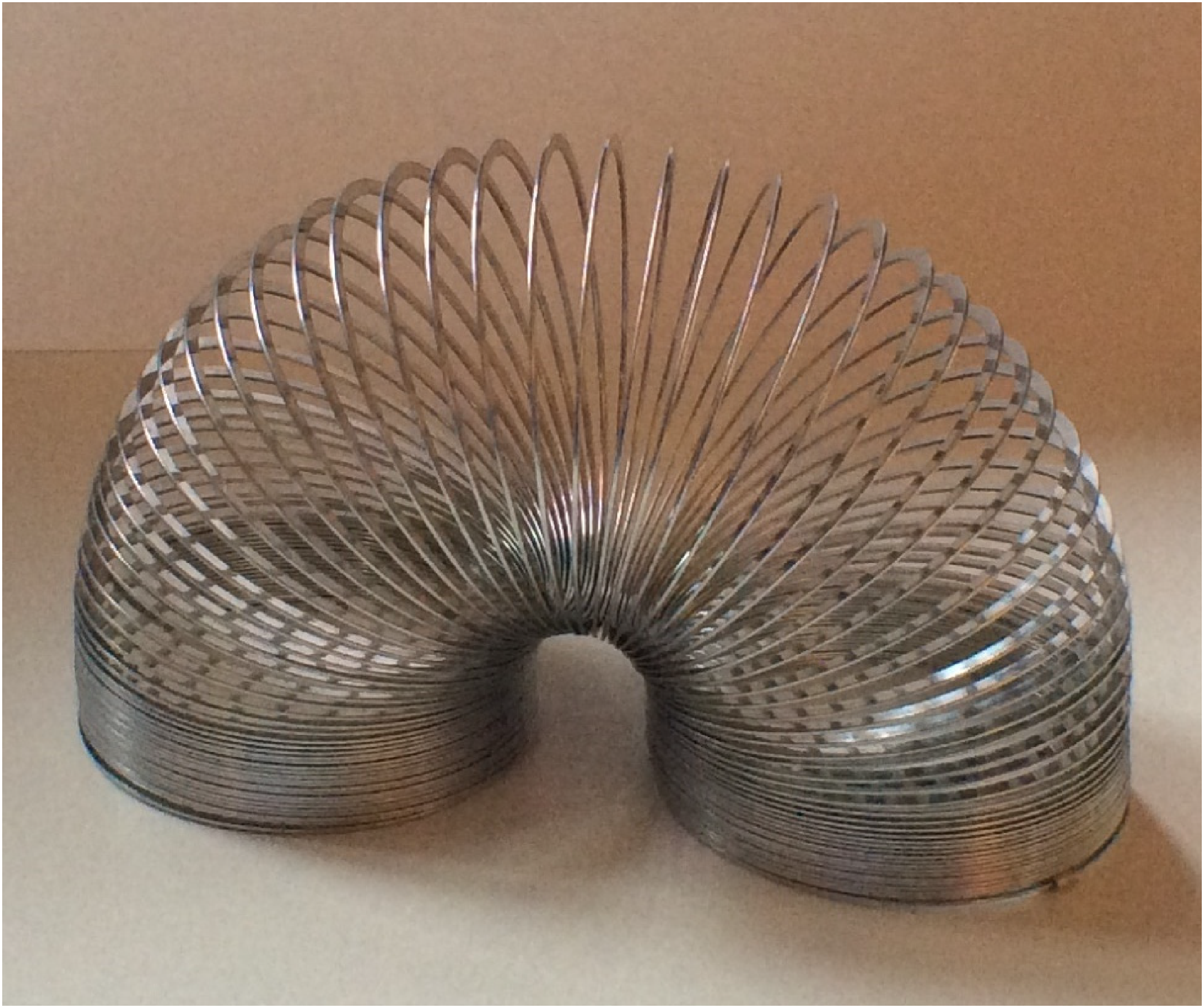
A Slinky in an arch configuration. ⁴

A Slinky can be made from plastic or metal and typically is formed into 35–75 coils of the spring. There are many demonstration videos on the internet. There are some experimental investigations of a Slinky in the open literature reviewed by Wilson. ⁵ Theoretical investigations or the modelling of a Slinky's dynamics are limited, see further discussion in the literature review section below. This paper presents a complete multi-body dynamics model of a Slinky that has the potential to qualitatively reproduce all aspects of the dynamic behavior discussed above.

Literature review

For the past three to four decades a weakness in mathematical skills of undergraduates joining science and engineering degree programs is an accepted phenomenon.^6–9 This is a particular issue for mechanical engineering students taking courses in mechanics and machine dynamics. The basis of these courses is Newton's 2nd law and requires a sound understanding of calculus, the formulation and solution of differential equations, vector analysis and the ability to formulate and manipulate equations. As well as identifying the issue, there has been much work to address the problem.

As the principal issue in dynamics is the motion of mechanical devices it make sense to use animation to demonstrate the solution of dynamical systems.^10,11 Animations make a strong link between the underlying equations of motion and the application of dynamics to real world systems. A use of multimedia in the teaching of dynamics is presented in Rohendi et al. ¹² Multimedia is also used in the teaching of dynamics where music generation from stringed instruments via the wave equation is demonstrated in Cumber. ¹³

Another approach to supporting students of dynamics is to provide a virtual learning environment (VLE) to solve the equations of motion for a particular mechanical engineering system. A VLE makes it possible to explore parameter space of a dynamical system without initially having a good understanding of the model's basis. The VLE also means that there is no requirement for any programming skills. Wideberg ¹⁴ produced a VLE for analyzing lateral vehicle dynamics. Another example of the application of a VLE is Silva et al. ¹⁵ where a GUI is used to simulate nonlinear dynamical systems.

There is a body of work where a device well known to the students, such as a simple pendulum is considered, and a deeper analysis is presented than an undergraduate student would usually experience.^16,17 In Cumber ¹⁷ it is shown that depending on the forcing conditions the unstable equilibrium configuration of a vertically up orientation of the pendulum becomes stable. It is also shown that the asymptotic state of a forced simple pendulum can bifurcate and through a sequence of bifurcations produce a chaotic trajectory. This counter-intuitive behavior can be very interesting to an undergraduate engineering student and encourage them to have a strong belief that dynamics is a mechanical engineering science that is worth investing time and effort into.

As discussed above there are many demonstrations on the internet of different physical phenomena using a Slinky. There is also a body of work discussing how a Slinky can be used in the education of physics and engineering students.^2,18–20 Considering theoretical studies of a Slinky the only model for a stair descending Slinky is derived by Hu. ²¹ The Slinky is represented as two bars linked in the middle. Up until recently the only multi-body dynamic model is one based on linear springs.^22,23 In the multi-body linear spring model, the Slinky is approximated as a sequence of point masses connected to each other by linear springs. The linear spring model can be thought of as a discrete analogue of the wave equation. It can reproduce the pseudo levitation property of a Slinky and some wave propagation behavior but cannot be extended to a stair descending Slinky. Holmes et al. ²⁴ produced a model for predicting static equilibrium for a Slinky. The Slinky is represented as a sequence of bars connected by springs that model the axial stress, shear stress and torsional stress. Holmes et al. ²⁴ state an intent to produce a dynamic model using this representation of a Slinky but as yet no model has been forthcoming. Cumber ⁴ calculated the static equilibrium for a Slinky by representing it as a sequence of half hoops connected by torsion springs, see Figure 2. For convenience this representation of a Slinky is labelled as the torsion spring model. The static equilibrium for the Slinky is calculated by minimizing the energy in the system subject to the boundary conditions and physical constraints. The advantage of the torsion spring/ half hoop representation is that it can be used as a basis for deriving a dynamic model for a Slinky. 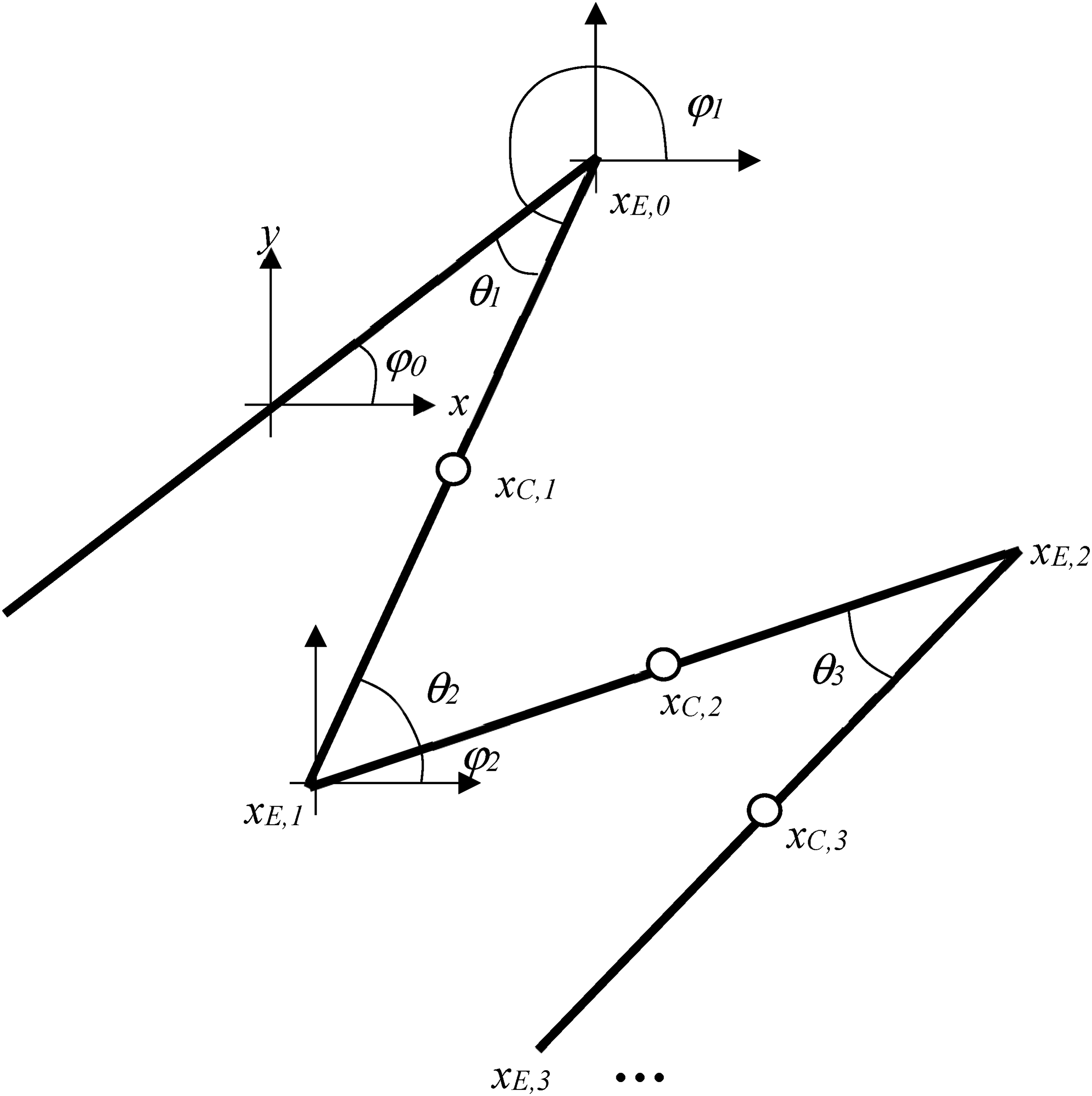²⁵ The parameters determining the kinematics for the half hoops of the Slinky are given in Figure 3. The fundamental dependent variables are the torsion angles, θ_j. Note the topology of a Slinky places a constraint on the torsion angles,

$${\theta }_j\ge {\theta }_{min}={\tan }^{-1}\left({\displaystyle \frac{\mathrm{\Delta }}{2R}}\right)$$

(1)

where Δ is the thickness of a coil and R is the radius of a coil. In Cumber ²⁵ the dynamic model for a Slinky assumes the inequality (1) is not violated and Lagrange's method is used to derive the equations of motion. The model derived by not including the physical constraint on torsion angles is only applicable to Slinky's with a near vertical orientation. The torsion spring model presented in Cumber ²⁵ is a significant improvement on the linear spring/ point mass model as it has the potential to be extended to allow a Slinky to simulate stair walking. In this paper the torsion spring model is improved such that the physical constraint on torsion angles (1) is satisfied. The extended model is then applied to a number of different initial orientations of a Slinky that are not perturbations of a Slinky from a vertical orientation. The paper concludes by considering future application of the torsion spring model.

Figure 2.

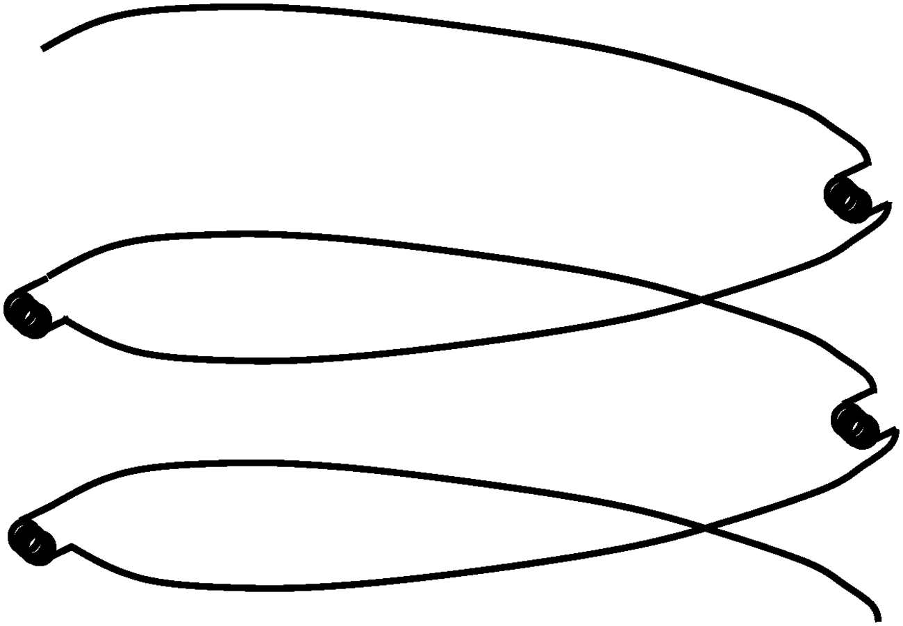
Schematic diagram showing a representation of a Slinky as a sequence of half hoops connected by torsion springs.

Figure 3.

Torsion spring model of a Slinky.

Torsion spring model

The basis of the Slinky model discussed here is a representation of a Slinky as a sequence of half hoops connected together by torsion springs, see Figure 2. In this section the torsion spring model is presented. It is separated into three parts.

The basis of the methodology for calculating the initial conditions of a Slinky is presented.

The equations of motion for a Slinky are derived.

The model for the impact of coils on each other is then discussed.

Initial condition for a Slinky

To describe the Slinky initial condition methodology, it is useful to define a number of sequencies required to describe the kinematics of a Slinky, see Figure 3. The location of the mid-point of each half coil $\{{\mathit{x}}_{\mathit{C},\mathit{k}}{\}}_{k=1}^{N_{coil}}$ and half hoop end points, $\{{\mathit{x}}_{\mathit{E},\mathit{k}}{\}}_{k=1}^{N_{coil}+1}$ , and the torsion angles, $\{{\theta }_k{\}}_{k=1}^{N_{coil}}$ are defined in Figure 3. It is useful to define the composite torsion angles as,

$${\mathrm{\Theta }}_k={\phi }_0+\sum _{j=1}^k{\theta }_j(-1{)}^{j+1}$$

(2)

where φ₀ defines the orientation of the Slinky base. The composite torsion angles can then be used to define the location of the half hoops.

$$\begin{array}{rl}& {\mathit{x}}_{\mathit{E},\mathit{k}+1}=x_{E,k}+2R\left(\begin{array}{c}\cos {\mathrm{\Theta }}_k\\ \sin {\mathrm{\Theta }}_k\end{array}\right)(-1{)}^k\\ & {\mathit{x}}_{\mathit{C},\mathit{k}+1}={\mathit{x}}_{\mathit{C},\mathit{k}}+R\left(\begin{array}{c}\cos {\mathrm{\Theta }}_k-\cos {\mathrm{\Theta }}_{k+1}\\ \sin {\mathrm{\Theta }}_k-\sin {\mathrm{\Theta }}_{k+1}\end{array}\right)(-1{)}^k\end{array}$$

(3)

where R is the radius of a half hoop. The repeated application of (3) gives the following expression for the vertical coordinates of the half hoops,

$$y_{C,k}=R\left(\sin {\mathrm{\Theta }}_0+2\sum _{j=1}^{k-1}\sin {\mathrm{\Theta }}_j{(-1)}^j+\sin {\mathrm{\Theta }}_k{(-1)}^k\right)$$

(4)

More details of the kinematics and the derivations of (2–4) are discussed further in Cumber.⁴

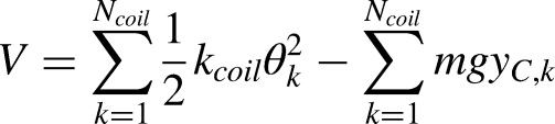
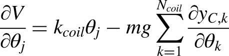
The energy of a stationary Slinky is the summation of the elastic potential energy of the torsion springs and the gravitational potential energy of the half hoops.

$$E=\sum _{i=1}^{N_{coil}}{\displaystyle \frac{1}{2}{k}_{coil}{\theta }_i^2+\sum _{j=1}^{N_{coil}}mg{y}_{C,j}}$$

(5)

where k_coil is a torsion spring constant. The static equilibrium condition for a Slinky fixed at one end is the minimization of the energy. The conditions for a local minimum are,

$$\begin{array}{rl}& {\displaystyle \frac{dE}{d{\theta }_i}=0}\\ & k_{coil}{\theta }_i+mg\sum _{j=1}^{N_{coil}}{\displaystyle \frac{d{y}_{C,j}}{d{\theta }_i}=0i=1,2,\dots ,N_{coil}}\end{array}$$

(6)

$${\displaystyle \frac{d{y}_{C,j}}{d{\theta }_i}=\left\{\begin{array}{cc}0& i>j\\ -R\cos {\mathrm{\Theta }}_j& i=j\\ R\left(2\sum _{k=i}^{j-1}\cos {\mathrm{\Theta }}_k{(-1)}^{k-i+1}+\cos {\mathrm{\Theta }}_j{(-1)}^{j-i+1}\right)& i<j\end{array}\right\}}$$

For a Slinky fixed at both ends the problem becomes a constrained optimization problem, where the energy is minimized subject to the end conditions and the physical constraint (1). This can be solved using a penalty method ²⁶ and requires the minimization of the object function labelled as the augmented energy.

$$f_{obj}(\mathit{\theta })=E_A=E+P_{{\theta }_{min}}+P_b$$

$$P_{{\theta }_{min}}={\alpha }_{min}\sum _{k=1}^{N_{coil}}\{max(0,-({\theta }_k-{\theta }_{min})){\}}^2$$

$$P_b={\alpha }_b\sum _{k=N_{coil}}^{N_{coil}+1}(x_{E,k}-x_{b,k}).(x_{E,k}-x_{b,k})$$

(7)

where α_min and α_b must be prescribed. The numerical optimization problem is solved using a quasi-Newton method.^27,28 There are multiple local minimizers of the Slinky energy. To find the correct minimum a continuation method is applied. The influence of the end constraint (7) is initially switched off, α_b= 0 and a sequence of optimization problems are solved with α_b being incrementally increased until the end condition is satisfied. If a continuation method is not used it is possible for a minimizer to be found where the Slinky shape can develop with an unwanted full rotation in it. Further details of the methodology are given in Cumber. ⁴

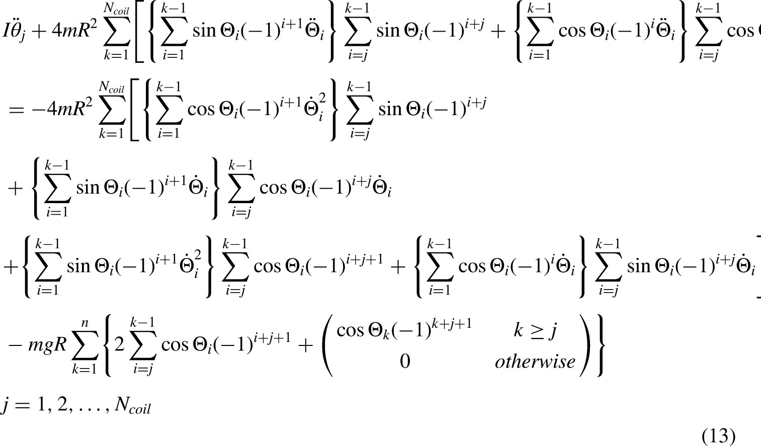
Equations of motion

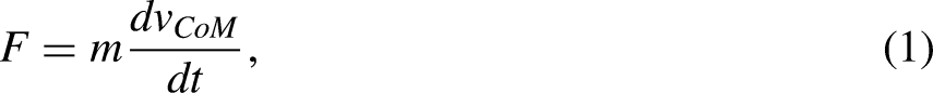
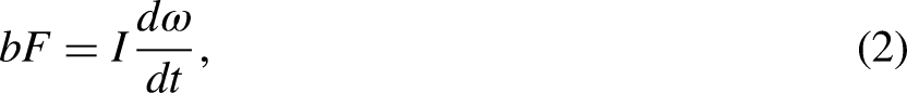
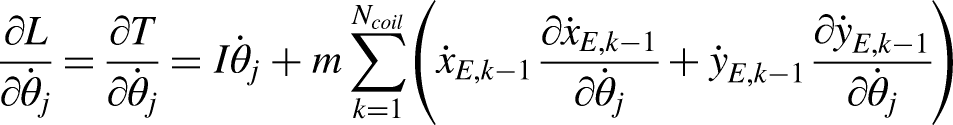
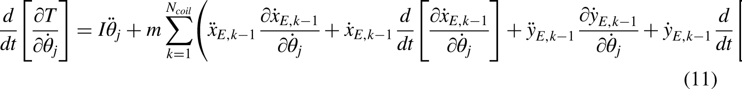
For the present the physical constraint (1) is not considered as part of the derivation of the model for the Slinky motion. The equations of motion are derived using the Lagrange method. The Lagrangian is defined as,

$$L=T-V$$

(8)

where T represents the kinetic energy of the system and V is the sum of the elastic potential energy and gravitational potential energy in the system,

$$T=\sum _{k=1}^{N_{coil}}{\displaystyle \frac{1}{2}I{\dot{\theta }}_k^2+\sum _{k=1}^{N_{coil}}{\displaystyle \frac{1}{2}m({\dot{x}}_{C,k}^2+{\dot{y}}_{C,k}^2)}}$$

(9)

$$V=\sum _{k=1}^{N_{coil}}{\displaystyle \frac{1}{2}{k}_{coil}{\theta }_k^2-\sum _{k=1}^{N_{coil}}mg{y}_{C,k}}$$

The equations of motion for the multi-body system are defined using the Lagrangian as

$${\displaystyle \frac{d}{dt}\left\{{\displaystyle \frac{\mathrm{\partial }L}{\mathrm{\partial }{\dot{\theta }}_j}}\right\}=-{\displaystyle \frac{\mathrm{\partial }L}{\mathrm{\partial }{\theta }_j}j=1,2,\dots ,N_{coil}}}$$

(10)

It remains to express the equations of motion in terms of independent variables such that the numerical solution using an ODE solver can be calculated.

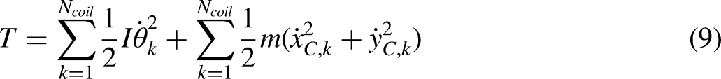
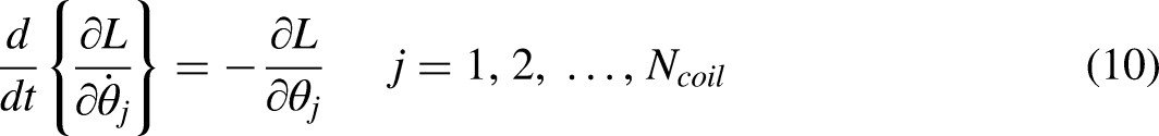
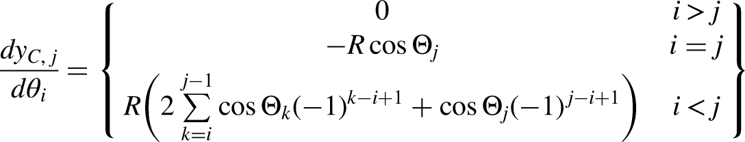
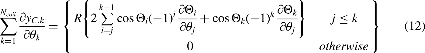
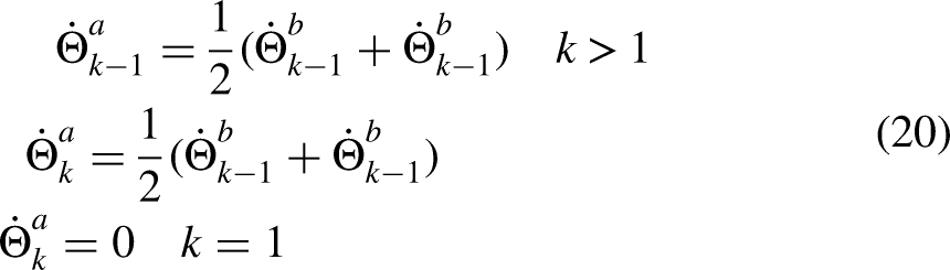
Using product and chain rule differentiation applied to (3, 4) it can be shown that terms in the equations of motion expressed as (10) are

$${\displaystyle \frac{\mathrm{\partial }L}{\mathrm{\partial }{\dot{\theta }}_j}={\displaystyle \frac{\mathrm{\partial }T}{\mathrm{\partial }{\dot{\theta }}_j}=I{\dot{\theta }}_j+m\sum _{k=1}^{N_{coil}}\left({\dot{x}}_{E,k-1}{\displaystyle \frac{\mathrm{\partial }{\dot{x}}_{E,k-1}}{\mathrm{\partial }{\dot{\theta }}_j}+{\dot{y}}_{E,k-1}{\displaystyle \frac{\mathrm{\partial }{\dot{y}}_{E,k-1}}{\mathrm{\partial }{\dot{\theta }}_j}}}\right)}}$$

$$\begin{array}{r}{\displaystyle \frac{d}{dt}\left[{\displaystyle \frac{\mathrm{\partial }T}{\mathrm{\partial }{\dot{\theta }}_j}}\right]=I{\ddot{\theta }}_j+m\sum _{k=1}^{N_{coil}}\left({\ddot{x}}_{E,k-1}{\displaystyle \frac{\mathrm{\partial }{\dot{x}}_{E,k-1}}{\mathrm{\partial }{\dot{\theta }}_j}+{\dot{x}}_{E,k-1}{\displaystyle \frac{d}{dt}\left[{\displaystyle \frac{\mathrm{\partial }{\dot{x}}_{E,k-1}}{\mathrm{\partial }{\dot{\theta }}_j}}\right]+{\ddot{y}}_{E,k-1}{\displaystyle \frac{\mathrm{\partial }{\dot{y}}_{E,k-1}}{\mathrm{\partial }{\dot{\theta }}_j}+{\dot{y}}_{E,k-1}{\displaystyle \frac{d}{dt}\left[{\displaystyle \frac{\mathrm{\partial }{\dot{y}}_{E,k-1}}{\mathrm{\partial }{\dot{\theta }}_j}}\right]}}}}\right)}\end{array}$$

(11)

Similarly applying the chain rule and product differentiation to the potential energy term, V.

$${\displaystyle \frac{\mathrm{\partial }V}{\mathrm{\partial }{\theta }_j}=k_{coil}{\theta }_j-mg\sum _{k=1}^{N_{coil}}{\displaystyle \frac{\mathrm{\partial }{y}_{C,k}}{\mathrm{\partial }{\theta }_k}}}$$

$$\sum _{k=1}^{N_{coil}}{\displaystyle \frac{\mathrm{\partial }{y}_{C,k}}{\mathrm{\partial }{\theta }_k}=\left\{\begin{array}{cc}R\left\{2\sum _{i=j}^{k-1}\cos {\mathrm{\Theta }}_i{(-1)}^i{\displaystyle \frac{\mathrm{\partial }{\mathrm{\Theta }}_i}{\mathrm{\partial }{\theta }_j}+\cos {\mathrm{\Theta }}_k{(-1)}^k{\displaystyle \frac{\mathrm{\partial }{\mathrm{\Theta }}_k}{\mathrm{\partial }{\theta }_j}}}\right\}& j\le k\\ 0& otherwise\end{array}\right\}}$$

(12)

Substituting for all Cartesian coordinate expressions using the composite torsion angle expression (2) and grouping all second order derivatives on one side gives the system of differential equations,

$$\begin{array}{rl}& I{\ddot{\theta }}_j+4m{R}^2\sum _{k=1}^{N_{coil}}\left[\left\{\sum _{i=1}^{k-1}\sin {\mathrm{\Theta }}_i{\left(-1\right)}^{i+1}{\ddot{\mathrm{\Theta }}}_i\right\}\sum _{i=j}^{k-1}\sin {\mathrm{\Theta }}_i{\left(-1\right)}^{i+j}+\left\{\sum _{i=1}^{k-1}\cos {\mathrm{\Theta }}_i{\left(-1\right)}^i{\ddot{\mathrm{\Theta }}}_i\right\}\sum _{i=j}^{k-1}\cos {\mathrm{\Theta }}_i{\left(-1\right)}^{i+j+1}\right]\\ & =-4m{R}^2\sum _{k=1}^{N_{coil}}[\left\{\sum _{i=1}^{k-1}\cos {\mathrm{\Theta }}_i{\left(-1\right)}^{i+1}{\dot{\mathrm{\Theta }}}_i^2\right\}\sum _{i=j}^{k-1}\sin {\mathrm{\Theta }}_i{\left(-1\right)}^{i+j}\\ & +\left\{\sum _{i=1}^{k-1}\sin {\mathrm{\Theta }}_i{\left(-1\right)}^{i+1}{\dot{\mathrm{\Theta }}}_i\right\}\sum _{i=j}^{k-1}\cos {\mathrm{\Theta }}_i{\left(-1\right)}^{i+j}{\dot{\mathrm{\Theta }}}_i\\ & +\left\{\sum _{i=1}^{k-1}\sin {\mathrm{\Theta }}_i{\left(-1\right)}^{i+1}{\dot{\mathrm{\Theta }}}_i^2\right\}\sum _{i=j}^{k-1}\cos {\mathrm{\Theta }}_i{\left(-1\right)}^{i+j+1}+\left\{\sum _{i=1}^{k-1}\cos {\mathrm{\Theta }}_i{\left(-1\right)}^i{\dot{\mathrm{\Theta }}}_i\right\}\sum _{i=j}^{k-1}\sin {\mathrm{\Theta }}_i{\left(-1\right)}^{i+j}{\dot{\mathrm{\Theta }}}_i]-k_{coil}{\theta }_j\\ & -mgR\sum _{k=1}^n\left\{2\sum _{i=j}^{k-1}\cos {\mathrm{\Theta }}_i{\left(-1\right)}^{i+j+1}+\left(\begin{array}{cc}\cos {\mathrm{\Theta }}_k{\left(-1\right)}^{k+j+1}& k\ge j\\ 0& otherwise\end{array}\right)\right\}\\ & j=1,2,\dots ,N_{coil}\end{array}$$

(13)

The solution variables are the composite torsion angles. The initial value problem is closed when the initial Slinky location/ orientation is given, and it is assumed that the Slinky is initially stationary.

$$\mathbf{\Theta }(0)={\mathbf{\Theta }}_{stdy}$$

$$\dot{\mathbf{\Theta }}(0)=\left(\begin{array}{c}\begin{array}{c}0\\ 0\\ ⋮\\ 0\end{array}\end{array}\right)$$

(14)

Note the torsion angles can be recovered from the composite torsion angles as,

$${\theta }_j=\{\begin{array}{c}\begin{array}{cc}{\mathrm{\Theta }}_1-{\phi }_0& j=1\end{array}\\ \begin{array}{cc}({\mathrm{\Theta }}_j-{\mathrm{\Theta }}_{j-1}){(-1)}^{j+1}& j>1\end{array}\end{array}$$

(15)

The model (13) can be represented as,

$$A(\mathbf{\Theta })\ddot{\mathbf{\Theta }}=f(\mathbf{\Theta },\dot{\mathbf{\Theta }})$$

(16)

which after further manipulation to produce a 1st order differential system can be solved using an ODE numerical solver based on a 4th/5th order Runge Kutta method. ²⁹ Further details of the derivation can be found in Cumber. ²⁵ The above system is complicated, but the derivation relies on concepts and processes that mechanical engineering students will be familiar with, such as the Lagrangian, chain rule differentiation and product differentiation. Where an engineering student would struggle is the manipulation of the system of equations into a manageable form. The model for a Slinky as a simulation tool is a useful thing for motivating students in the study of machine dynamics. An engineering student would understand the starting point of the analysis and the numerical solution at the end point of the process, but the derivation in the middle requires a significant investment in time and effort.

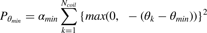
In Cumber ²⁵ the above model is applied to Slinkies with a vertical or near vertical orientation. The model works well for N_coil≤ 15 but for the larger Slinky's is unstable due to round off error. This is investigated in Cumber ²⁵ and found to be due to an energy imbalance that grows with time for N_coil of twenty or more. To address this an energy dissipation term is added to the system.

$$A(\mathbf{\Theta })\ddot{\mathbf{\Theta }}=f(\mathbf{\Theta },\dot{\mathbf{\Theta }})-C_D\dot{\mathit{\theta }}$$

(17)

where C_D is given a small positive value. In a real system there is energy dissipation but here it is used to prevent false energy generation. This means that the model should be qualitatively correct and is valid for a finite time interval.

Modelling coil impacts

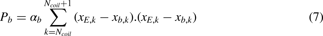
To extend the range of application of the Slinky model the impact of half coils adjacent to one another must be accounted for. The approach taken is one based on conservation of momentum and the theory of inelastic collision of bodies. Detection of one of these impact events is straightforward. If there is an impact between two half coils the impact condition is,

$$\begin{array}{cc}{\theta }_k={\theta }_{min}& {\dot{\theta }}_k<0\end{array}$$

(18)

When (18) is satisfied the ODE solver is stopped and the state $({\mathbf{\Theta }}^{\mathit{a}},{\dot{\mathbf{\Theta }}}^{\mathit{a}})$ must be modified in someway to produce a new initial value problem. The superscripts b and a indicate quantities before and after impact. Treating the impact as an inelastic collision with a zero coefficient of restitution the two half hoops after impact have the same velocity or the relative velocity $v_{k-1,k}^a$ is zero.

$$v_{k-1,k}^a=R{\dot{\theta }}_k^a=0$$

(19)

In composite torsion angle space conservation of momentum gives the expressions,

$$\begin{array}{c}\begin{array}{cc}{\dot{\mathrm{\Theta }}}_{k-1}^a={\displaystyle \frac{1}{2}({\dot{\mathrm{\Theta }}}_{k-1}^b+{\dot{\mathrm{\Theta }}}_{k-1}^b)}& k>1\end{array}\\ \begin{array}{c}{\dot{\mathrm{\Theta }}}_k^a={\displaystyle \frac{1}{2}({\dot{\mathrm{\Theta }}}_{k-1}^b+{\dot{\mathrm{\Theta }}}_{k-1}^b)}\\ \begin{array}{cc}{\dot{\mathrm{\Theta }}}_k^a=0& k=1\end{array}\end{array}\end{array}$$

(20)

The extension of the Slinky model ²⁵ requires the solution of a number of initial value problems. In the next section the simulation of Slinky's with initial conditions that are remote from a near vertical orientation is considered.

Simulations and analysis

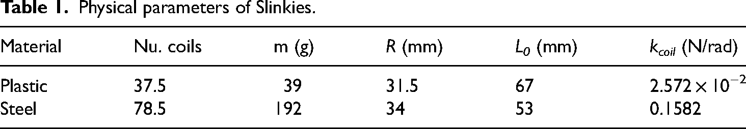
The Slinkies used in this study are defined in Table 1. The spring constants, k_coil are calibrated to give the correct length of a Slinky in a vertical steady state orientation. In this section five simulations are considered, four simulations of the plastic Slinky with different initial conditions and the final simulation is a metal Slinky. In all simulations the Slinky is taken to be attached to a fixed point at the origin.

Table 1.

Physical parameters of Slinkies.

Material	Nu. coils	m (g)	R (mm)	L0 (mm)	kcoil (N/rad)
Plastic	37.5	39	31.5	67	2.572 × 10−2
Steel	78.5	192	34	53	0.1582

Plastic Slinky simulations

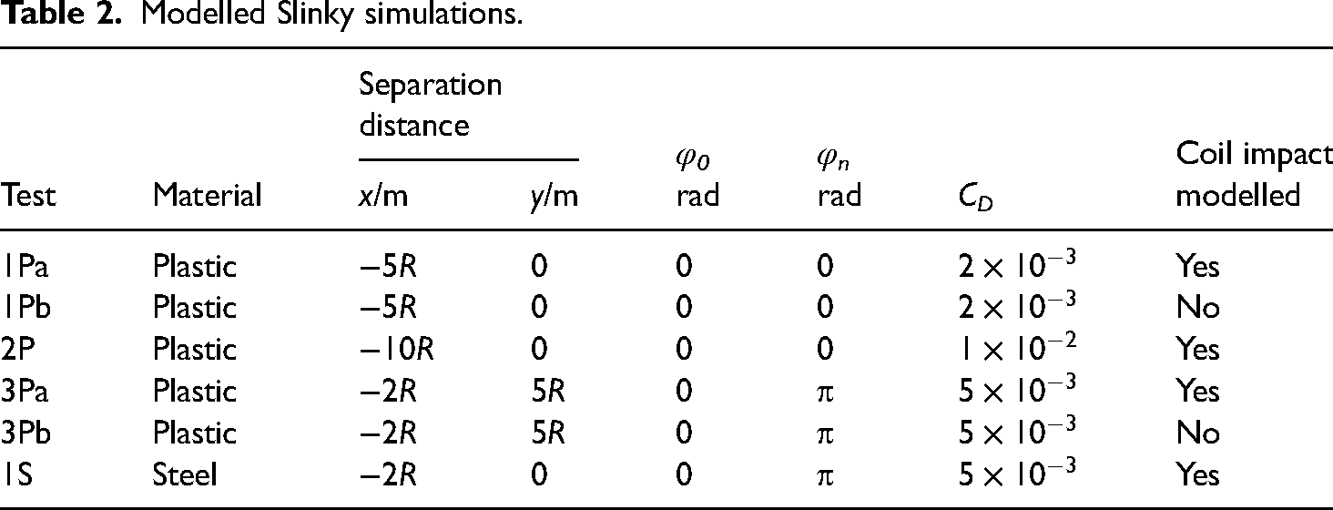
The four plastic Slinky simulations are defined in Table 2. In the first simulation, Test 1Pa, coil impacts are modelled, and the initial Slinky distribution is defined by the Slinky having a downward orientation, φ₀= 0 rad with the center of the Slinky base initially located at (−5R, 0). The Slinky base at (−5R, 0) is released at t = 0 s. In Figure 4 the Slinky location at t = 0, 0.2, …, 1.4 s is plotted. The Slinky initially contracts due to the spring tension and descends under the action of gravity. The Slinky rotates anticlockwise and extends to a maximum vertical location of approximately y = −0.65 m. For times of 0.8 s through to 1.4 s the predicted sense of rotation changes with the Slinky contracting vertically. At the end of the simulation, t = 1.4 s the Slinky has contracted to a vertical location of approximately y = −0.25 m.

Figure 4.

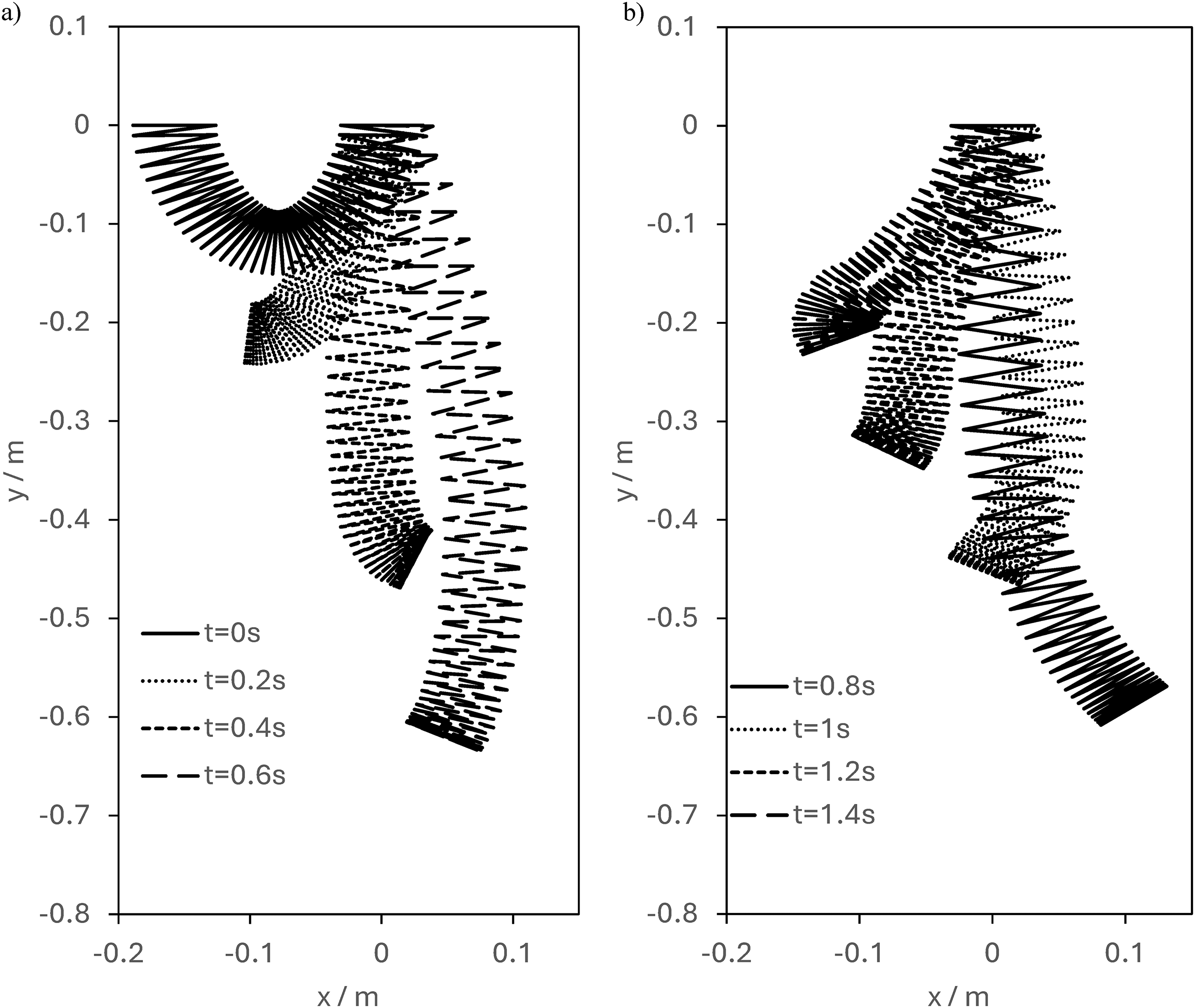
Simulation of a plastic Slinky, test 1Pa, coil impacts modelled (a) 0 ≤ t ≤ 0.6 s, and (b) 0.8 ≤ t ≤ 1.4 s.

Table 2.

Modelled Slinky simulations.

Test	Material	Separation distance		φ0	φn	CD	Coil impact modelled
		x/m	y/m	rad	rad
1Pa	Plastic	−5R	0	0	0	$2\times {10}^{-3}$	Yes
1Pb	Plastic	−5R	0	0	0	$2\times {10}^{-3}$	No
2P	Plastic	−10R	0	0	0	$1\times {10}^{-2}$	Yes
3Pa	Plastic	−2R	5R	0	π	$5\times {10}^{-3}$	Yes
3Pb	Plastic	−2R	5R	0	π	$5\times {10}^{-3}$	No
1S	Steel	−2R	0	0	π	$5\times {10}^{-3}$	Yes

Test 1Pb is the same simulation conditions as Test 1Pa apart from coil impacts are not modelled. For Test 1Pb the predicted Slinky trajectory is shown in Figure 5. The same time-slices as shown for Test 1Pa, t = 0., 0.2, …, 1.4 s are presented. Comparing Figures 4 and 5 the overall evolution of the Slinky trajectories is similar. For t = 0.4 s the base of the Slinky in Figure 5 shows evidence of negative torsion angles, violating (1), for some values of j, but neglecting coil impacts seem to be a second order effect. This will be investigated for other Slinky configurations.

Figure 5.

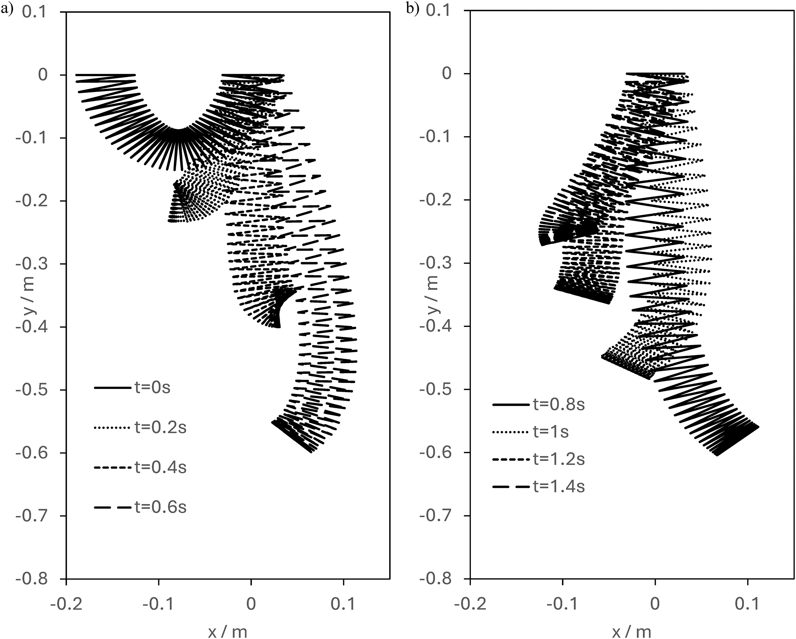
Simulation of a plastic Slinky, test 1Pb, coil impacts not modelled (a) 0 ≤ t ≤ 0.6 s, and (b) 0.8 ≤ t ≤ 1.4 s.

The second initial configuration is a Slinky with the center of the Slinky base initially located at (−10R, 0), Test 2P. This doubles the separation distance compared to Test 1Pa and due to the dependency of the elastic potential energy on the distortion of the spring is 4 times the first configuration, Test 1Pa. Figure 6 shows the evolution of a Slinky for Test 2P. The same time-slices as the simulation, Test 1Pa, t = 0, 0.2, …, 1.4 s are shown. Comparing Figure 6 with Figure 4 there is more lateral motion with anticlockwise rotation until t = 0.8 s when the sense of rotation changes. One difference for Test 2P compared to Test 1Pa is there is much less extension of the Slinky. The maximum extension of the Slinky is y = −0.4 m. The reason for the difference is that although the Slinky is modelled as a sequence of torsion springs and half coils organized in series, the orientation of the half coils can produce a notional spring force perpendicular to the half coils. For Test 2P the nontrivial spring force has a more horizontal direction compared to Test 1Pa. For Test 1Pa there is a more vertical extension in the -y direction than for Test 2P.

Figure 6.

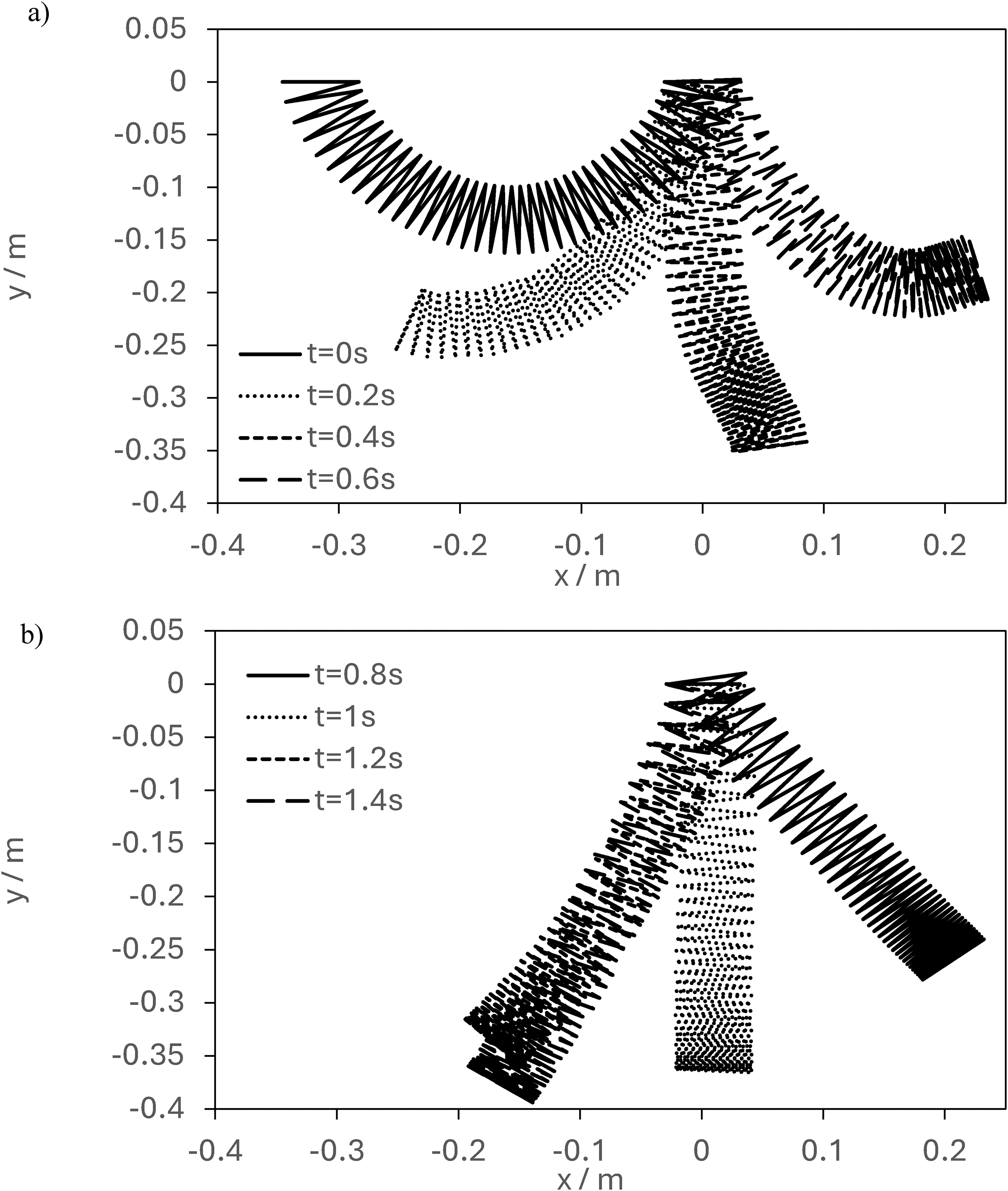
Simulation of a plastic Slinky, test 2P, coil impacts modelled (a) 0 ≤ t ≤ 0.6 s, and (b) 0.8 ≤ t ≤ 1.4 s.

The final initial plastic Slinky configuration considered is a Slinky with the center of the Slinky base located at (−2R, 5R). The Slinky orientation at (−2R, 5R) is, φ_n= π, this is different to Test 1Pa and Test 2P. This configuration is of interest as the initial shape is more complex than investigated previously. Figure 7 shows the Slinky evolution for Test 3Pa. In this simulation the methodology for modelling coil impacts is implemented. The same time-slices, t = 0, 0.2, …, 1.4 s are shown in Figure 7 as shown for Test 1Pa, Test 1Pb and Test 2P.

Figure 7.

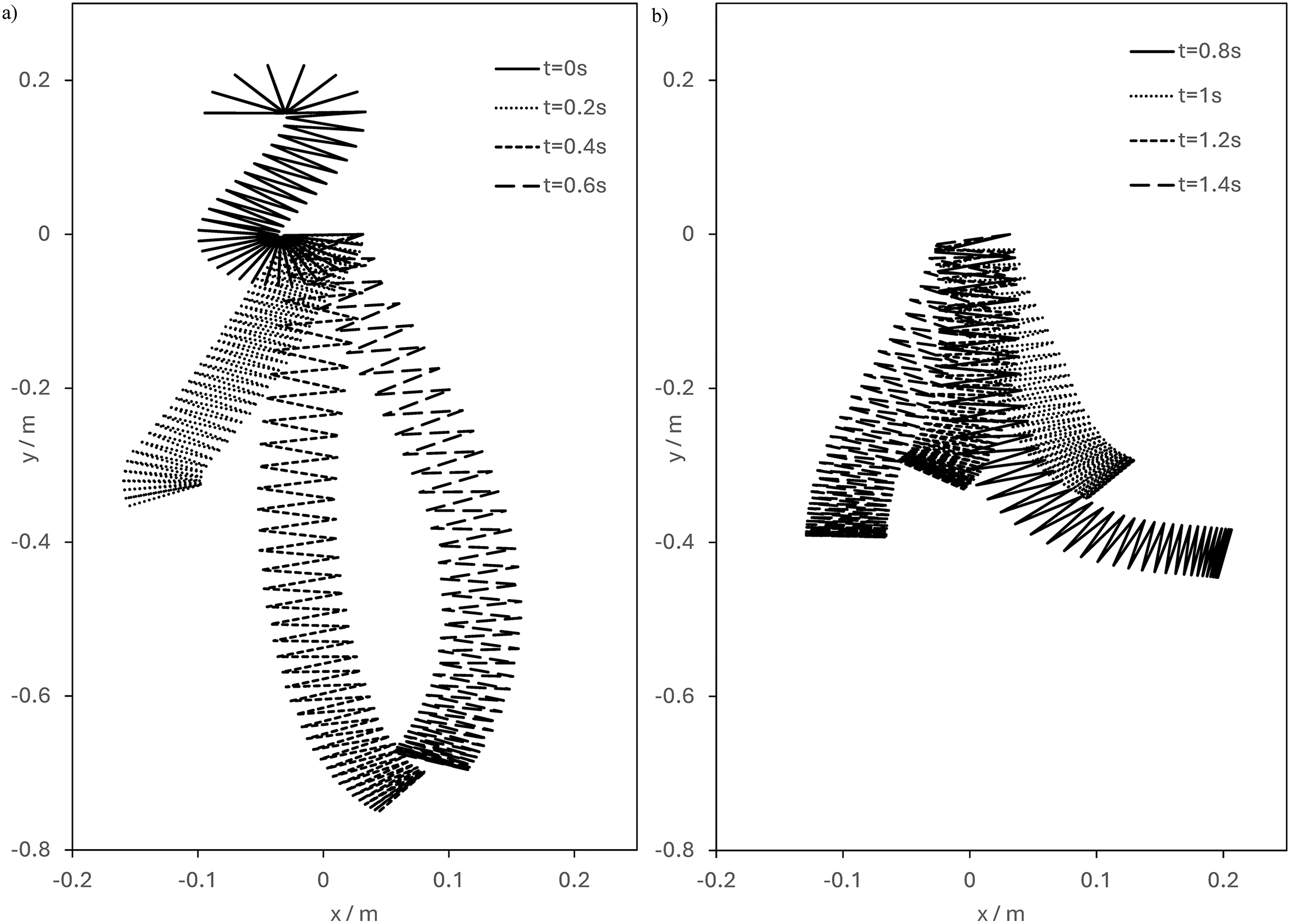
Simulation of a plastic Slinky, test 3Pa, coil impacts modelled (a) 0 ≤ t ≤ 0.6 s, and (b) 0.8 ≤ t ≤ 1.4 s.

For Test 3Pa, in the simulation the Slinky extends to y = −0.75 m at t = 0.6 s and for later times the Slinky contracts to y = −0.4 m and oscillates with a swaying motion for t > 0.4 s. One final plastic Slinky simulation, Test 3Pb is shown in Figure 8. Every part of the Slinky specification is the same as Test 3Pa except coil impacts are not modelled. The results of the simulation shown in Figure 8 should be compared with Figure 7. Unlike Test 1Pa and Test 1Pb ignoring the coil impacts does significantly change the Slinky trajectory.

Figure 8.

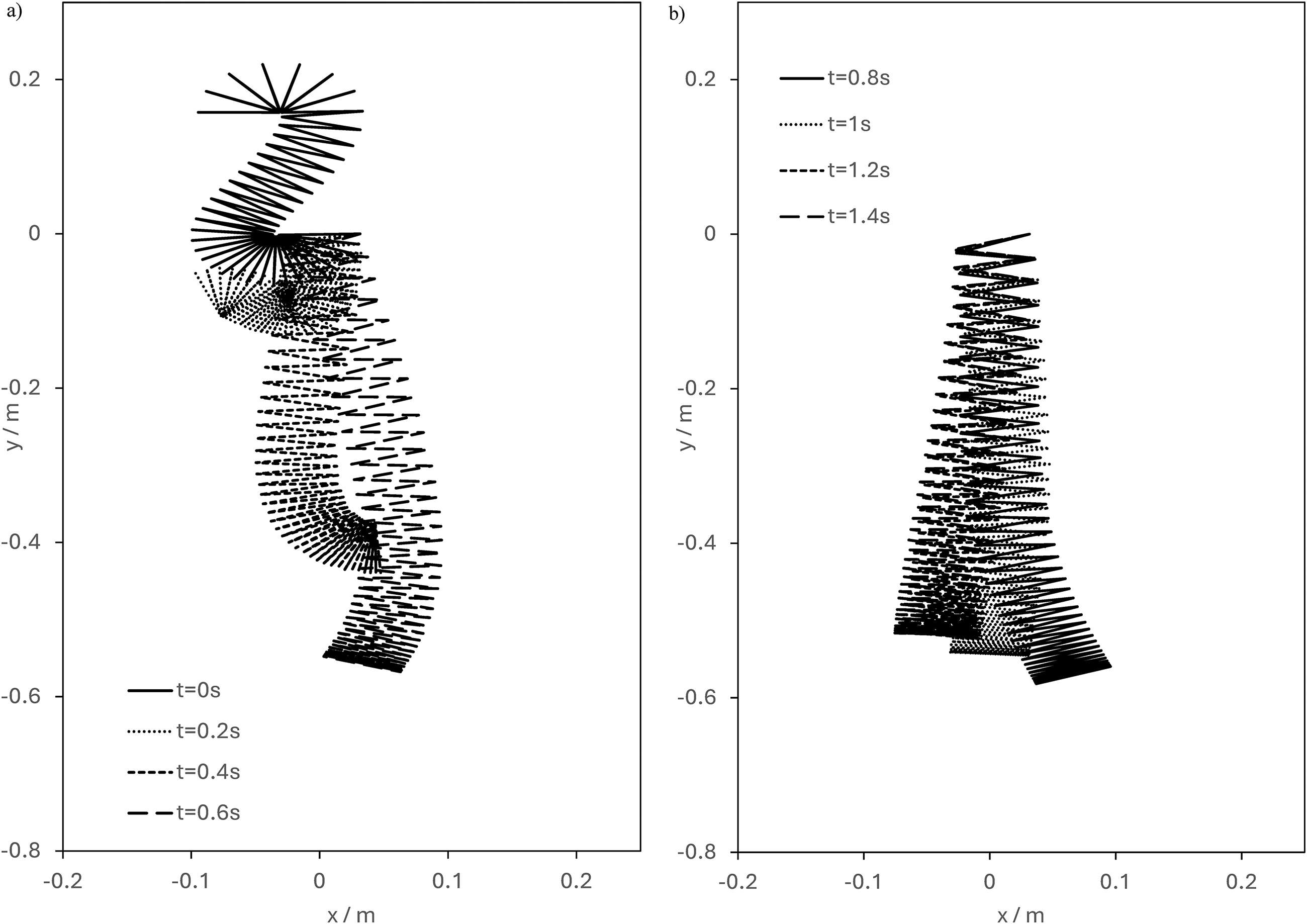
Simulation of a plastic Slinky, test 3Pb, coil impacts not modelled (a) 0 ≤ t ≤ 0.6 s, and (b) 0.8 ≤ t ≤ 1.4 s.

In summary the tests, Test 1Pb and Test 3Pb indicate that neglecting coil on coil impacts is an increasing problem with increases in initial energy in the system. As the initial energy in the Slinky is increased coil on coil impact has a larger effect on the overall motion of the Slinky. For Test 1Pb the overall orientation and trajectory of the Slinky is similar to Test 1Pa, see Figures 4 and 5. For Test 3Pa and Test 3Pb the Slinky has more energy than Test 1Pa and Test 1Pb. For Test 3Pa and Test 3Pb neglecting coil on coil impact changes the Slinky trajectory significantly, see Figures 7 and 8.

Steel Slinky

For the steel Slinky simulation, Test 4S the center of the base of the Slinky is located at (−2R, 5R) and the orientation of the base is φ_n= π. This is the same initial orientation as Test 3Pa. In Figure 9 the Slinky trajectory is given for time-slices t = 0, 0.4, …, 1.6 s. Due to the coil mass spring constant values the Slinky trajectory evolves to a near vertical oscillation very quickly. To show the second order effects in the Slinky evolution the x-axis for each of the Slinky time-slices is given as x + Δx t where Δx = 0.25 m/s. The introduced origin shift makes it easier to interpret the simulation as the overall Slinky location in space is similar for all time slices for t > 0.4 s. The trajectory of the steel Slinky shows that it evolves away from its initial configuration very quickly, for t > 0.4 s the Slinky oscillates vertically. An inspection of Figure 9 shows the steel Slinky has a second order lateral oscillation superimposed on the vertical oscillation.

Figure 9.

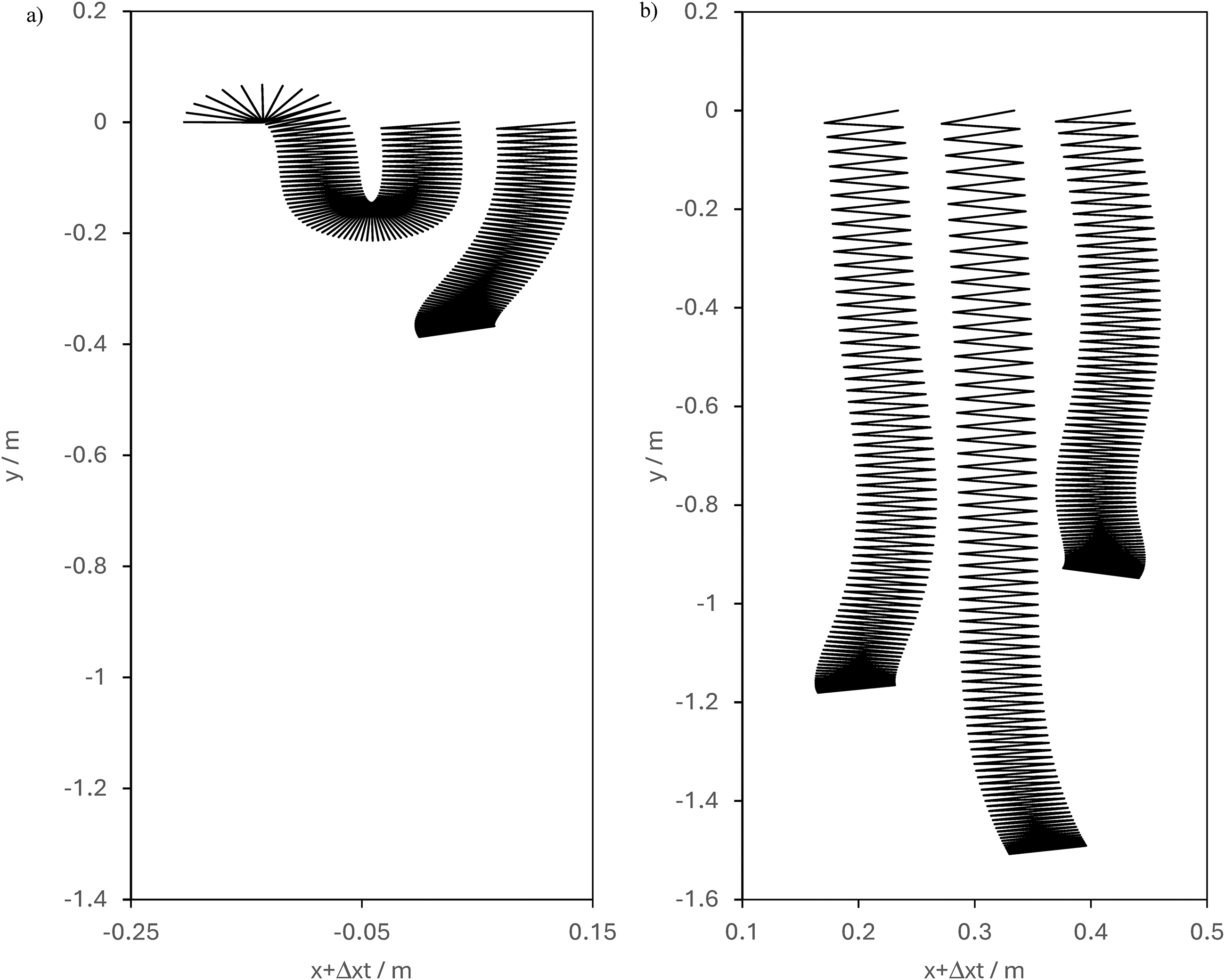
Simulation of a steel Slinky, test 4S, coil impacts modelled (a) t = 0 and t = 0.4 s, and (b) t = 0.8, 1.2 and 1.6 s.

Enhancing the student experience

A Slinky can be used to demonstrate a range of phenomena, such as stair walking, pseudo gravity, propagation of longitudinal waves, propagation of transverse waves and resonance.

The previously accepted model based on linear springs can simulate some aspects of Slinky behavior, such as pseudo gravity but is not universal. The torsion spring model in principle can be applied to all the above Slinky behavior. As with most dynamical systems the phenomena can be exhibited using animation of the simulations. The animation of the linear spring model is insightful but requires some imagination to make the connection with a Slinky. The torsion spring Slinky model has the advantage that representing a Slinky as a series of half hoops connected by torsion springs looks like a Slinky and moves in a similar way to a Slinky. This makes the animation of a torsion spring Slinky model animation more accessible than the linear spring model.

When considering how the torsion spring Slinky model could be incorporated into the student experience the following are some of the possible ways forward. The torsion spring Slinky model could be used in support of physical demonstrations of a Slinky's motion. For example, pseudo gravity is about the finite time of transmission of information down the Slinky. Using the torsion spring model, it is possible to compute the information propagation speed.

The formulation of the torsion spring Slinky model uses concepts such as Lagrange's method, that are typically part of the syllabus on an advanced dynamics undergraduate course. This makes it appropriate to be a computational model demonstration in an advanced course in dynamics. It is also useful as a ‘beacon’ to early undergraduate years students of introductory or intermediate courses in dynamics as a demonstration of what is possible.

Another enhancement of the student experience would be to implement the torsion spring model with a GUI. The GUI implementation of the model could then be given to the students to give them an opportunity to explore parameter space for Slinky simulations of their choice. This would be particularly useful if the students are organized into small groups. This would promote discussion and interaction between students and with the lecturer.

Conclusion

A torsion spring model is extended to be applicable to a wide range of initial Slinky configurations. The original torsion spring model could only be applied to situations where coil to coil impact is not significant. This restricted the initial Slinky configuration to be a near vertical orientation only. The torsion spring model is extended by modelling coil to coil impacts as inelastic impacts with a coefficient of restitution of zero. The complete torsion spring model is applied to several different initial Slinky shapes. The dynamic behavior is demonstrated to be qualitatively correct for two different Slinky's.

The derivation of the torsion spring model is a complicated model to derive but once rearranged into an appropriate form is relatively straight forward to solve numerically. It is a dynamic system that nearly all undergraduate engineering students will be familiar with. Their experience of it could be to do with its stair walking property or other physical phenomena. It is not argued that an engineering student should be able to derive the torsion spring model, although it is constructed using mathematical techniques and constructs well known to students. It is argued that the student's familiarity with a Slinky and its fundamental physical simplicity and its tactile nature make a model of its dynamics very appealing and engaging. The torsion spring model is an example of a dynamic model that can be used to demonstrate to the undergraduate engineering cohort what is possible in the application of dynamics to a mechanical device they are familiar with.

The torsion spring model can qualitatively reproduce the evolution of a Slinky and can be used to investigate many physical phenomena of relevance to the dynamics of a Slinky. The torsion spring model of a Slinky has reached a level of maturity such that it can now be a basis for investigating other Slinky dynamic phenomena. The model can be used to investigate longitudinal and transverse wave propagation. Forcing a Slinky means that resonance can be investigated in an unusual way compared to the typical model used for demonstrating resonance, the forced simple pendulum.^16,17

The model can be used to simulate the pseudo-levitation property of Slinky's. Finally with minor modification the torsion spring model can be used to investigate stair walking from a theoretical perspective. There are a number of questions regarding the Slinky propagation velocity as a function of Slinky parameters and stair parameters that could be investigated.

A final issue is the quantitative validation of the torsion spring model. This will require an experimental program that will involve the design of a stair rig, and the use of video image analysis based on the digital image correlation technique.