
Abstract
Optimal component tolerances can reduce product cost and improve enterprise competitiveness. In order to obtain optimal tolerances accurately and efficiently, analytical methods are applied to solve tolerance optimization model. In this article, both manufacturing cost and quality loss are included in the total cost, and two kinds of constraints, including assembly tolerance constraint and process accuracy constraints, are considered in the tolerance optimization model. In order to allocate the optimal tolerances among the related components, the following procedure is presented. First, the two kinds of constraints are ignored, and analytical method is applied to find the initial values of component tolerances. If the initial component tolerances cannot satisfy assembly tolerance constraint, the Lagrange multiplier method is executed and the Lambert W function is applied to solve the corresponding equations to obtain the new values of component tolerances. Then, process accuracy constraints are satisfied through the adjustment of component tolerances. Finally, an example is used to demonstrate the effectiveness of the method proposed in this article.
Introduction
Because the component tolerances have significant influence on production cost, tolerance design becomes an important part of product development. Tighter tolerance would result in high manufacturing cost, while looser tolerance may lead to poor performance. Therefore, component tolerance should be optimized, and this issue has received the attention of many researchers in the last decades.
In these works about tolerance design, an important issue is how to establish the proper relationship between the manufacturing cost and tolerance. In order to establish cost–tolerance function, first, the discrete manufacturing cost data should be obtained. Then, curve-fitting techniques are adopted to fit the discrete data, and proper mathematical model is obtained. Over the past decades, many cost–tolerance functions have been proposed. These cost functions proposed prior to 1990 are referred to as traditional cost functions, while those proposed after 1990 are named as nontraditional cost functions. 1 Wu et al. 2 and Chase et al. 3 introduced several traditional cost functions, such as reciprocal function, reciprocal square function, reciprocal power function, exponential function, reciprocal power and exponential hybrid function, linear function, and piecewise linear function. Dong et al. 4 proposed several nontraditional cost functions, including combined reciprocal powers and exponential function, combined linear and exponential function, B-spline curve function, cubic polynomial function, fourth-order polynomial function, and fifth-order polynomial function.
In the early studies about tolerance optimization, only manufacturing cost was considered and tolerance was optimized to minimize manufacturing cost.2–5 In these years, quality loss has attracted more attention.6–16 In order to estimate monetary loss incurred by poor product’s performance, Taguchi et al. 6 proposed quality loss function, which is a quadratic function. At present, the sum of manufacturing cost and quality loss is usually treated as the objective function in the studies about tolerance optimization.7–16
When tolerance optimization models are established, suitable methods should be employed to obtain optimal tolerances. Over the past decades, a number of numerical optimization methods were adopted to calculate optimal tolerances, including nonlinear programming, 9 integer programming, 10 genetic algorithm, 11 continuous ant colony algorithm, 12 particle swarm optimization,13,14 hybrid of simplex method and particle swarm optimization algorithm, 15 self-organizing migration algorithm, 16 and so on.
Although numerical methods have been widely used in tolerance optimization, analytical method should be the first choice because of its high efficiency and accuracy. In fact, the Lagrange multiplier method seems to be the oldest analytical method for constrained nonlinear programming problems. 1 Because the Lagrange multiplier method can generate closed-form optimal solution, it has been studied by a few of researchers.1–3,11,17,18 Chase et al. 3 modeled the manufacturing cost–tolerance characteristics using reciprocal power function and assembly tolerance constraint using root-sum-square method. In the model proposed by Spotts, 17 the manufacturing cost functions were represented using reciprocal square function, and both the worst-case method and root-sum-square method were applied to establish assembly tolerance constraints. Singh et al. 11 and Kumar and Stalin 18 used exponential cost function and worst-case model. Although Lagrange multiplier method has obtained the attention of these researchers, some limitations exist in these studies: (1) Quality loss was not included in the objective function and (2) process accuracy constraints were not studied.
Jeang 19 and Shin et al. 20 considered quality loss in their objective function and applied calculus-based analytical method to obtain the optimal tolerances. However, assembly tolerance constraint was not studied in their research.
In this article, analytical method is executed to obtain the optimal tolerance to minimize the sum of manufacturing cost and quality loss. Both assembly constraint and process accuracy constraints are included in the model proposed in this article, and closed-form solution of optimal tolerance is derived.
Model formulation
Manufacturing cost
In this article, the exponential function is used to model the manufacturing cost, and the total manufacturing cost associated with a mechanical assembly can be addressed as
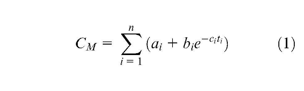
where n is the number of components in the assembly, coefficients ai, bi, and ci are unique for each component, and ti is the tolerance of component i.
Quality loss cost
Based on Taguchi’s standpoints, the expected quality loss cost can be computed by
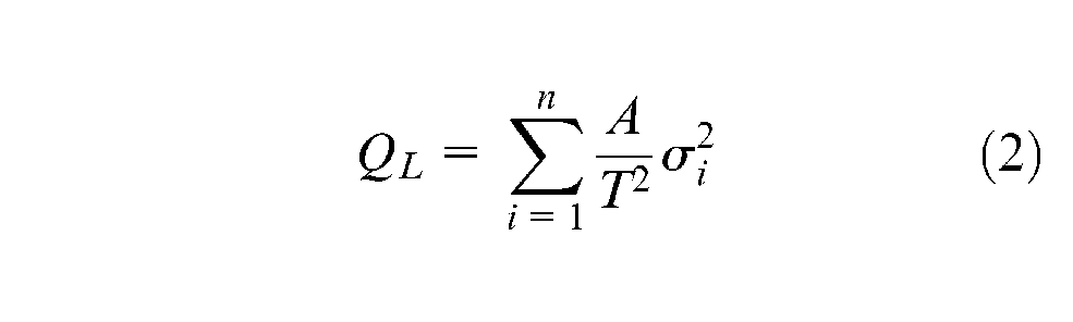
where A is quality loss coefficient, T is the single-side functional tolerance stack up limit for the assembly dimension chain, and
Then, the expected quality loss can be rewritten as follows
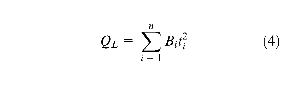
where
Total cost
In this article, the objective function is the total cost, which includes manufacturing cost and quality loss
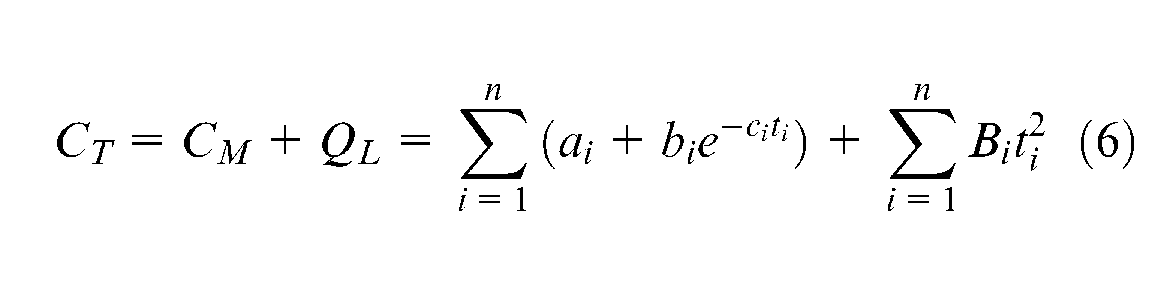
The total cost, manufacturing cost, and quality loss cost are shown in Figure 1. It can be found that the minimum total cost can be obtained at the optimal tolerance
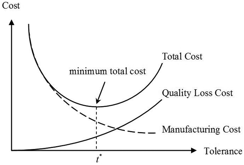
Cost–tolerance curve.
Design constraints
Assembly tolerance constraint
Over the past decades, a few of tolerance analysis methods have been applied to establish assembly tolerance constraint, and worst-case method and root-sum-square method are the two most widely used methods. Based on the worst-case method, the assembly tolerance constraint can be written as follows
where
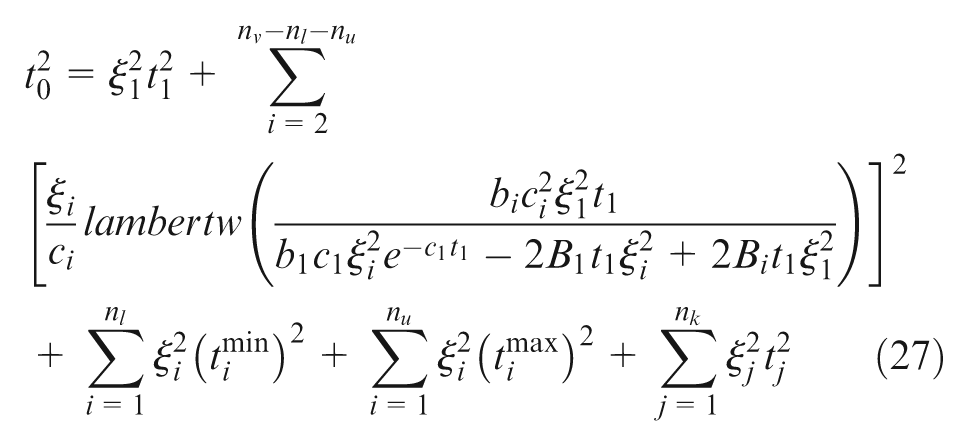
where nv is the number of component tolerances that need to be calculated. Based on the root-sum-square method, assembly tolerance constraint can be established as follows
Equation (9) is based on the assumption that the distribution is normal with its mean centered at the nominal value.
Process accuracy constraints
Each component tolerance has its own limits
where
Analytical solution for optimal tolerance
In order to satisfy assembly tolerance constraint and process accuracy constraints, this article proposes the following procedure to calculate optimal tolerance.
Unconstrained tolerance optimization
First, both assembly tolerance constraint and process accuracy constraints are not considered, and analytical method is applied to find the minimum total cost by setting the first derivative of equation (6) to 0
The solution of equation (11) is
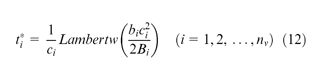
where Lambertw is Lambert W function,
21
and
Using equation (12), optimal tolerances
Optimal tolerance satisfying assembly tolerance constraint
In this article, both worst-case method and root-sum-square method are considered.
Worst-case method
Combining equations (6) and (8), the augmented system of equations is obtained
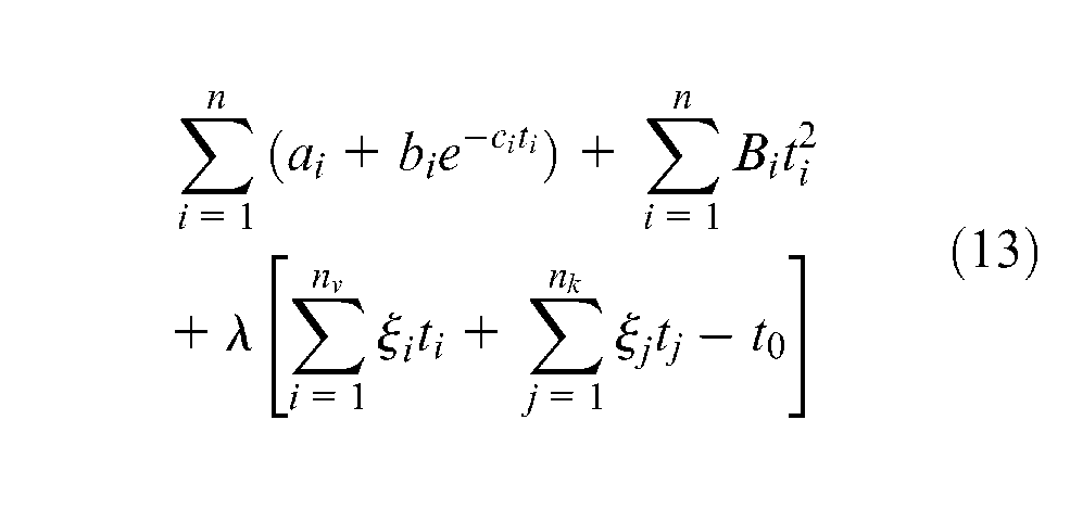
where
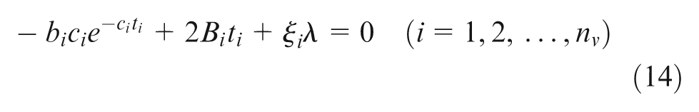
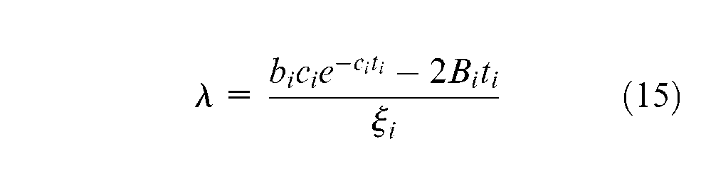
Eliminating
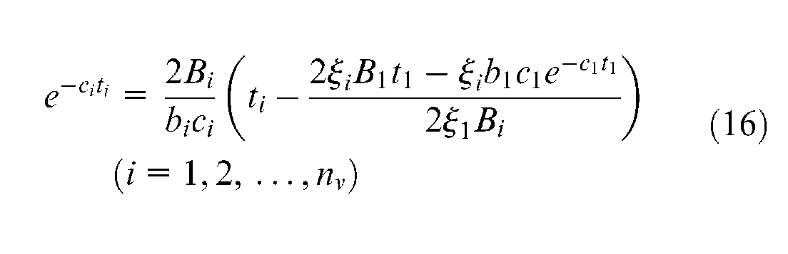
The solution of equation (16) is
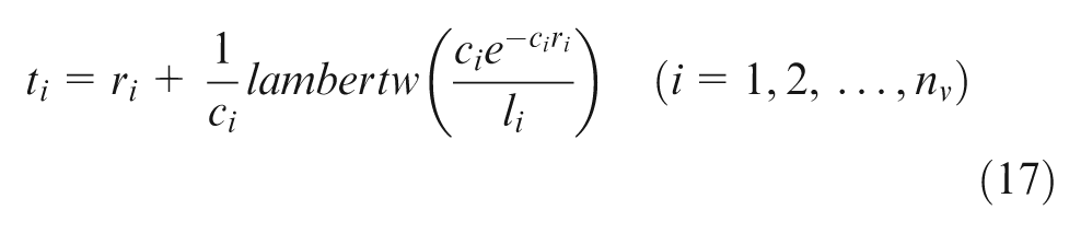
where
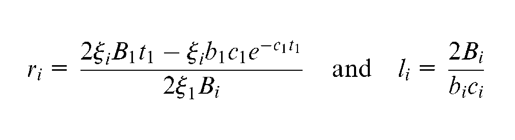
Substituting equation (17) into the corresponding assembly tolerance constraint, the following equation is established
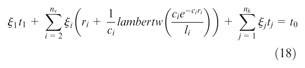
Equation (18) can be solved iteratively to determine t1, and other component tolerances ti can also be calculated using equation (17). Although the worst-case tolerances ti, which are obtained using equations (17) and (18), satisfy assembly constraint, it is not sure that they satisfy process accuracy constraints.
Root-sum-square method
Equations (6) and (9) are combined into an augmented system of equations
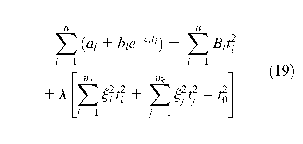
We set the first derivatives of equation (19) equal to 0
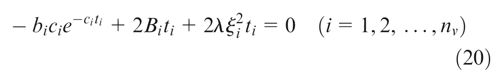
According to equation (20), the following relationships are established
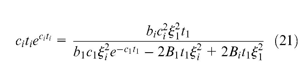
The solution of equation (21) is
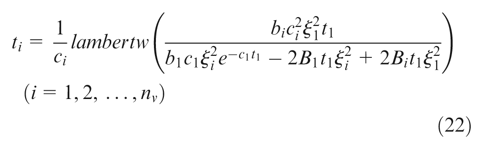
Equation (22) can be substituted into the corresponding assembly tolerance constraint
Equation (23) can be solved iteratively to determine t1, which can be substituted into equation (22) to obtain all component tolerance ti (
Optimal tolerance satisfying both assembly tolerance constraint and process accuracy constraints
In order to obtain the optimal tolerances satisfying both assembly tolerance constraint and process accuracy constraints, the following optimization procedure is proposed:
First, the initial values of optimal tolerances are calculated using equation (12), which are denoted by
If
If
If
If
Based on these two rules, component tolerances are determined in the first and third subsets.
Steps 1–3 are repeated sequentially until optimal tolerances of all components are obtained. Because the component tolerances have been determined in the first and third subsets, the component tolerances in the second subset should be optimized based on the following assembly tolerance constraint
Using equations (17) and (24), the following equation is established based on worst-case method
Using equations (22) and (25), the following equation is established based on the root-sum-square method
Solving equation (26) (or equation (27)), t1 is obtained, and other component tolerances can be calculated using equation (17) (or equation (22)).
According to the optimization procedure proposed in this article, the closed-form solution of optimal tolerance is obtained, which satisfy both assembly tolerance constraint and process accuracy constraints.
Illustrative example
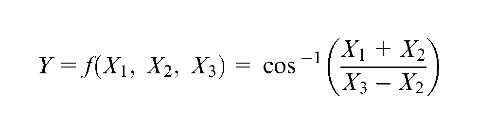
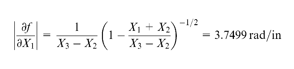
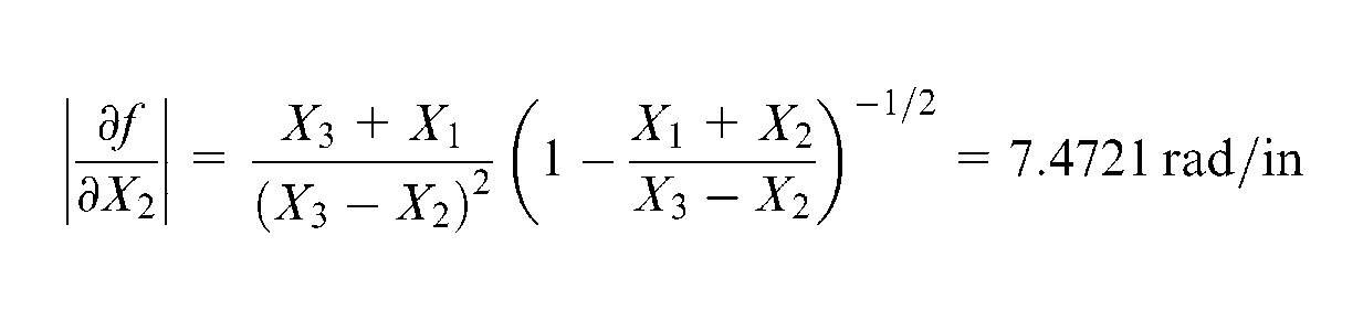
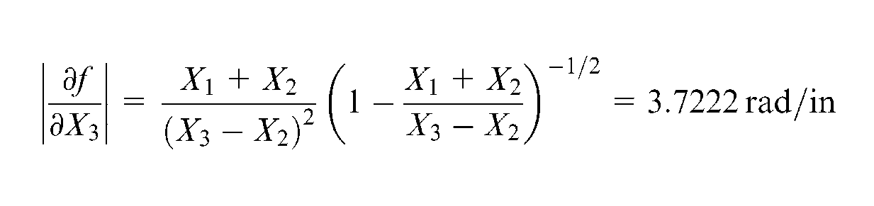
The overrunning clutch presented by Feng and Kusiak 10 is applied to demonstrate the effectiveness of the method proposed in this article. The clutch, which is shown in Figure 2, consists of three kinds of components: hub, roller, and cage, denoted by X1, X2, and X3, respectively. The contact angle Y is the assembly functional dimension
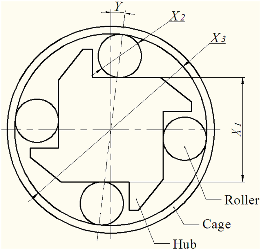
Overrunning clutch.
The normal value and the tolerance of contact angle Y are
Process accuracy constraints for these components are
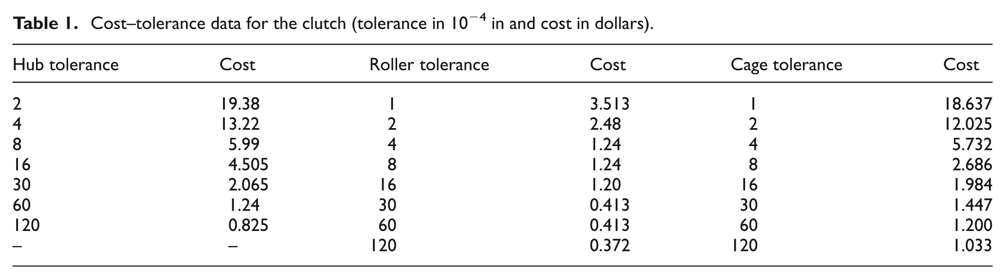
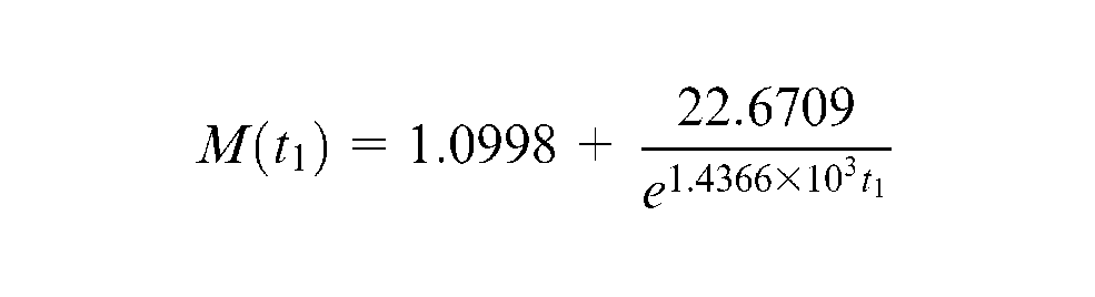
The cost–tolerance data proposed by Feng and Kusiak 10 are used in this article, which are illustrated in Table 1. Exponential function is applied to model manufacturing cost functions, which are obtained through curve fitting
Cost–tolerance data for the clutch (tolerance in 10−4 in and cost in dollars).
Quality loss cost is calculated as follows
The objective function is the sum of manufacturing cost and quality loss
subject to


Assuming quality loss coefficient A = 50, the optimal worst-case tolerances can be calculated as follows:
Using equation (12), the initial values of optimal tolerances are calculated as follows:
In order to satisfy assembly tolerance constraint, equations (17) and (18) are used to obtain the new values of optimal tolerances:
The tolerance of second component is adjusted to satisfy process accuracy constraints, and the following optimal tolerance is determined:
Because the optimal tolerance of the second component is determined, the tolerance of the first and third components should be calculated again to minimize the objective function. First, Step 1 is repeated to obtain the new value of component tolerances
Based on the method proposed in this article, the optimal tolerances are obtained and shown in Table 2. In order to demonstrate the effectiveness of the method proposed in this article, numerical optimization method is also used to resolve this problem, and the optimal tolerances are obtained and listed in Table 3.
Results obtained by the method proposed in this article (tolerance in inches and cost in dollars).
Results obtained by numerical method (tolerance in inches and cost in dollars).
The comparison of Tables 2 and 3 clearly indicates that the analytical method, which is proposed in this article, is more accurate than the numerical method, and improvement in the objective function (0.00000001, 0.00000003, 0.00000001, and 0.00000007) is found for different values of A (50, 100, 1000, and 5000). In fact, when A = 500, the objective functions obtained by the analytical method and the numerical method are equal to 11.4142586953 and 11.4142586972, respectively. Although the difference is very small and cannot be illustrated in Tables 2 and 3, the analytical method actually obtains smaller objective function. Tables 2 and 3 indicate that the assembly tolerance constraint does not influence the value of optimal worst-case tolerances, and only process accuracy constraints influence it. Therefore, the optimal statistical tolerances should be equal to the optimal worst-case tolerances.
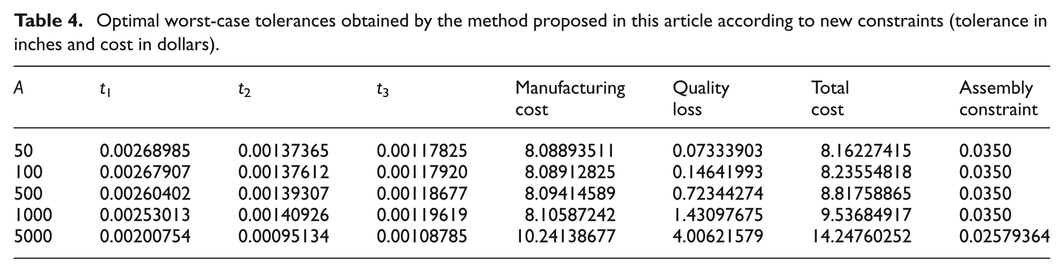
Tables 2 and 3 also indicate that the process accuracy constraint for the roller is overqualified. In order to reduce manufacturing cost, this article adjusts the process accuracy constraints for the roller, and the new process accuracy constraints for these components are
Optimal worst-case tolerances obtained by the method proposed in this article according to new constraints (tolerance in inches and cost in dollars).
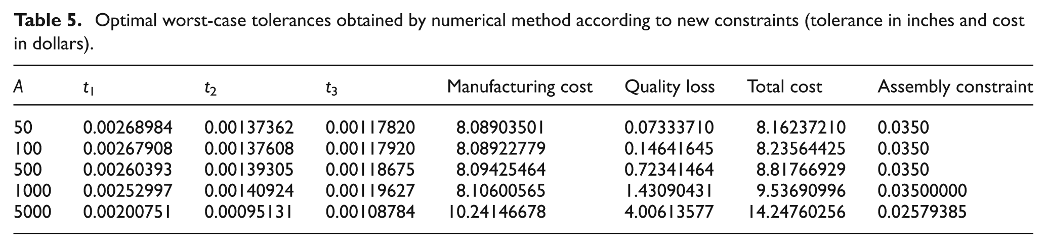
Optimal worst-case tolerances obtained by numerical method according to new constraints (tolerance in inches and cost in dollars).
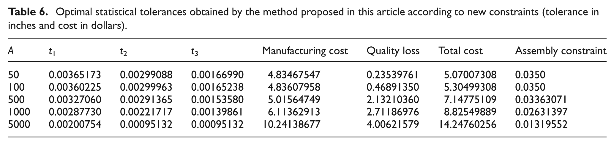
Optimal statistical tolerances obtained by the method proposed in this article according to new constraints (tolerance in inches and cost in dollars).
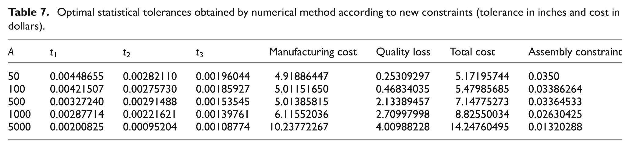
Optimal statistical tolerances obtained by numerical method according to new constraints (tolerance in inches and cost in dollars).
Conclusion
In order to minimize the sum of manufacturing cost and quality loss, the article proposes analytical methods to obtain closed-form solutions for the optimal tolerances, and all constraints, including assembly tolerance constraint and process accuracy constraints, are satisfied. Comparing with numerical method, both the computational efforts and the total cost are reduced. This demonstrates that the proposed method is indeed efficient and effective. It should be noted that the analytical method proposed in this article is only applicable to a few of manufacturing cost functions. In the future, the proposed method should be investigated to solve as many as tolerance optimization problems.
Footnotes
Declaration of conflicting interests
The authors declare that there is no conflict of interest.
Funding
This research received no specific grant from any funding agency in the public, commercial, or not-for-profit sectors.